A Comparative Study of Divergence Cleaning Methods of Magnetic Field in the Solar Coronal Numerical Simulation

This paper presents a comparative study of divergence cleaning methods of magnetic field in the solar coronal three-dimensional numerical simulation. For such purpose, the diffusive method, projection method, generalized Lagrange multiplier method and constrained-transport method are used. All these methods are combined with a finite-volume scheme in spherical coordinates. In order to see the performance between the four divergence cleaning methods, solar coronal numerical simulation for Carrington rotation 2056 has been studied. Numerical results show that the average relative divergence error is around 10^−4.5 for the constrained-transport method, while about 10^−3.1−10^−3.6 for the other three methods. Although there exist some differences in the average relative divergence errors for the four employed methods, our tests show they can all produce basic structured solar wind.

1. Introduction

Magnetohydrodynamics (MHD) equations are presently the only system available to self-consistently describe large-scale dynamics of space plasmas, and numerical MHD simulations has enabled us to capture the basic structures of the solar wind plasma flow and transient phenomena. The modern MHD codes can successfully solve both in time accurate and steady state problems involving all kinds of discontinuities. Different from the usual computational fluid mechanics, the MHD scheme has to be designed so as to guarantee the divergence free constraint of the magnetic field in two or three-dimensional MHD calculations. It is well-known that simply transferring conservation law methods for the Euler to the MHD equations can not be supposed to work at default in maintaining the divergence-free of magnetic field. The ∇ · B error accumulated during the calculation may grow in an uncontrolled fashion, which can result in unphysical forces and numerical instability (Tóth, 2000; Jiang et al., 2012a).

Several methods have been proposed to satisfy the ∇ · B = 0 constraint in MHD calculations. The eight-wave formulation approach, suggested by Powell et al. (1993, 1999), is to solve the MHD equations with the additional source terms that are proportional to ∇ · B without modifying the MHD solver. In this approach, divergence of the magnetic can be controlled to a truncation error and the robustness of a MHD code can be improved (Hayashi, 2005; Jiang et al., 2012a,b). The projection method was first proposed by Brackbill and Barnes (1980). In the projection method, the magnetic field B* provided by the base scheme in the new time step n + 1 is projected onto the subspace of zero divergence solutions by a linear operator, and the magnetic field in the new time step n + 1 is completed by this projected magnetic field solution (Brackbill and Barnes, 1980; Tóth, 2000; Balsara and Kim, 2004; Hayashi, 2005; Feng et al., 2010). Some authors (e.g., Brandenburg et al., 2008; Manabu et al., 2009) modify the MHD equations with the help of vector potential A instead of the magnetic field B = ∇ × A to keep divergence cleaning condition. In this case, ∇·(∇ × A) = 0 is guaranteed mathematically, such that solving the time evolution of the vector potential A maintains the magnetic field divergence-free during the time evolution. The diffusive method is to add a source term η∇(∇ · B) in the induction equation to reduce the numerical error of ∇ · B, so that the numerically generated divergence can be diffused away at the maximal rate limited by the CFL condition (van der Holst and Keppens, 2007; Feng et al., 2011; Shen et al., 2014). To guarantee the divergence cleaning of the magnetic fields, Dedner et al. (2002) proposed the hyperbolic divergence cleaning approach by introducing a generalized Lagrange multiplier (GLM). In the GLM method, a newly transport variable ψ is introduced to the MHD system, which plays the role of convecting the local divergence error out of the computational domain (Dedner et al., 2002, 2003; Mignone and Tzeferacos, 2010; Mignone et al., 2010; Jiang et al., 2012a,b; Susanto et al., 2013). The constrained transport (CT) method is a different strategy to control ∇ · B originally devised by Evans and Hawley (1988), in which the magnetic field is defined at face centers and the remaining fluid variables are provided at cell centers. In this approach, the electric field along the cell edges defining the boundary of the corresponding face is used to calculate the magnetic flux at cell faces. The CT method sustains a specified discretization of the magnetic field divergence around the machine round off error as long as the boundary and initial conditions are compatible with the constraints (Ziegler, 2011, 2012; Feng et al., 2014).

Since magnetic fields with a non-zero divergence can lead to severe artifacts in numerical simulations, keeping the magnetic field divergence-free is a curial problem in space plasma physics of solar and interplanetary phenomena. To say a few without exhausting, Linker et al. (1999) used the vector potential method to maintain the ∇ · B constraint for global solar corona simulations. Hayashi (2005) simulate the solar corona and solar wind using the eight-wave method and the projection method to reduce the nonphysical effects of ∇ · B. Jiang et al. (2012a,b) simulated the coronal and chromospheric microflares by adopting the eight-wave method and the extended generalized Lagrange multiplier (EGLM) method to clean the divergence error. The GLM method was used in a nonlinear force-free field (NLFFF) study for the dynamics of solar active region (Inoue et al., 2015). The eight-wave method, the projection method, the CT method and the GLM method were implemented (Tóth, 2000; Tóth et al., 2005, 2012; Feng et al., 2010, 2011, 2014; Shen et al., 2014) for solar coronal and heliospheric studies, so as to maintain the solenoidal constraint.

In this paper, we give a comparative study of divergence cleaning methods of magnetic field in the solar coronal numerical simulation. The CT method, the diffusive method, the projection method and the GLM method are used to maintain divergence constraint respectively. The 3D solar wind model (Feng et al., 2014) is used for the experiments. The code employed a semi-discrete central scheme, designed by Ziegler (2011, 2012) within an finite volume (FV) framework without a Riemann solver or characteristic decomposition, and a composite grid system in spherical coordinates without polar singularities (Feng et al., 2010, 2011, 2014).

This paper proceeds as follows. In Section 2, model equations and grid system for solar wind plasma in spherical coordinates are described. Section 3 introduces the four methods to maintain the divergence cleaning constraint on the magnetic field. Section 4 gives the initial and boundary conditions in the code. Section 5 presents the numerical results for the steady-state solar wind structure of Carrington rotation (CR) 2056. Finally, we present some conclusions in Section 6.

2. Governing Equations and Mesh Grid System

2.1. Governing Equations

The magnetic field B = B₁ + B₀ is splitted as a sum of a time-independent potential magnetic field B₀ and a time-dependent deviation B₁ (Feng et al., 2010, 2014). The MHD equations are splitted into the fluid and the magnetic parts. The governing equations have the same form as Feng et al. (2014). The fluid part of the vector $\text{U}={\left(\rho ,\rho v_r,\rho v_{\theta },\rho v_{\varphi }r sin \theta ,e\right)}^T$ reads as follows:

$\begin{array}{ll}\frac{\partial \text{U}}{\partial t}+\frac{1}{r^2}\frac{\partial }{\partial r}{r}^2\text{F}+\frac{1}{r sin \theta }\frac{\partial }{\partial \theta } sin \theta \text{G}+\frac{1}{r sin \theta }\frac{\partial }{\partial \varphi }\text{H}=\text{S}& (1)\end{array}$

The magnetic induction equation runs as follows:

$\begin{array}{l}\frac{\partial B_{1r}}{\partial t}+\frac{1}{r sin \theta }\frac{\partial }{\partial \theta }(sin \theta (v_{\theta }{B}_r-v_r{B}_{\theta }))-\frac{1}{r sin \theta }\frac{\partial }{\partial \varphi }\\ (v_r{B}_{\varphi }-v_{\varphi }{B}_r)=0& (2)\end{array}$

$\begin{array}{ll}\frac{\partial B_{1\theta }}{\partial t}-\frac{1}{r}\frac{\partial }{\partial r}(r(v_{\theta }{B}_r-v_r{B}_{\theta }))+\frac{1}{r sin \theta }\frac{\partial }{\partial \varphi }(v_{\varphi }{B}_{\theta }-v_{\theta }{B}_{\varphi })=0& (3)\end{array}$

$\begin{array}{ll}\frac{\partial B_{1\varphi }}{\partial t}+\frac{1}{r}\frac{\partial }{\partial r}(r(v_r{B}_{\varphi }-v_{\varphi }{B}_r))-\frac{1}{r}\frac{\partial }{\partial \theta }(v_{\varphi }{B}_{\theta }-v_{\theta }{B}_{\varphi })=0& (4)\end{array}$

Here, ρ is the mass density, v = (v_r, v_θ, v_ϕ) are the flow velocities in the frame rotating with the Sun, p is the thermal pressure. e stands for the modified total energy density consisting of the kinetic, thermal, and magnetic energy densities (written in terms of B₁).

2.2. Mesh Grid System

Following Feng et al. (2010, 2012a,b,c), the computational domain is divided into a composite mesh consisting of six identical component meshes designed to envelop a spherical surface with partial overlap on their boundaries (Figure 1).

FIGURE 1

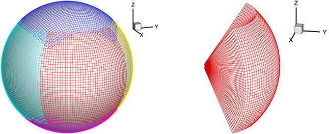
Figure 1. Partition of a sphere into six identical components with partial overlap (left) and one-component mesh stacked in the r direction (right).

In the present work, the parallel implementation over the whole computational domain from 1 R_s to 26 R_s is realized by domain decomposition of six-component grids based on the spherical surface and radial direction partition. The following grid partitions are employed: N_θ = N_ϕ = 42.Δr(i) = 0.01 R_s if r(i) < 1.1 R_s; Δr(i) = min(A × log₁₀(r(i − 1)), Δθ × r(i − 1)) with A = 0.01∕log₁₀(1.09) if r(i) < 3.5 R_s; Δr(i) = Δθ × r(i − 1) if r(i) > 3.5 R_s.

3. Numerical Scheme Formulation

The following four subsections are devoted to the introduction of four methods to maintain the divergence cleaning constraint on the magnetic field.

3.1. CT Method

By the usage of a special discretization of the magnetic field Equations (2)–(4), CT technique imitates the analytical fact that $\frac{\partial \nabla ·\text{B}}{\partial t}=\nabla ·\nabla \times (\text{v} \times \text{B})=0$. This discretization is routinely made on a particular stencil, therefore employs a staggered mesh, over which the solenoidal constraint up to the machine accuracy is satisfied on condition that initially ∇ · B = 0 is met in the whole computational domain. The hydrodynamic state variables are evaluated at the cell center, whereas magnetic field is evaluated at the cell faces and the electric field is at the cell edges. The origin of this technique is attributed to the staggered divergence-free scheme formulated for electromagnetism by Yee (1966). For spatial discretization of our numerical scheme formulation, we strictly follow those of Feng et al. (2014) by using the FV discretization of Equation (1), and by averaging Equations (2)–(4) over facial areas to obtain the semi-integral forms of magnetic induction equations. Second-order accurate linear ansatz reconstruction are adopted.

3.2. Diffusive Method

The diffusive method in maintaining the divergence-free constraint runs as follows. As usual, regarding the coupling of fluids and magnetic fields as a whole system, then we have

$\begin{array}{r}\text{ U}={\left(\rho ,\rho v_r,\rho v_{\theta },\rho v_{\varphi }r sin \theta ,e,B_{1r},B_{1\theta },B_{1\varphi }\right)}^T\\ \frac{\partial \text{U}}{\partial t}+\frac{1}{r^2}\frac{\partial }{\partial r}{r}^2\text{F}+\frac{1}{r sin \theta }\frac{\partial }{\partial \theta } sin \theta \text{G}+\frac{1}{r sin \theta }\frac{\partial }{\partial \varphi }\text{H}=\text{S}& (5)\end{array}$

with the symbols having their routine meanings, three variables added into Equation (1), and the first five variables keeping the same.

We use the diffusive method proposed to handle the ∇ · B constraint. A source term η∇(∇ · B) is introduced in the induction equation to reduce the numerical error of ∇ · B. The ∇ · B error produced by the diffusive method is controlled by iterating

$\begin{array}{l}{\text{B}}^{n+1}={\text{B}}^{n+1}+\eta \Delta t\nabla (\nabla ·{\text{B}}^{n+1})\end{array}$

$\eta \Delta t\le C_d{\left(\frac{1}{{(\Delta r)}^2}+\frac{1}{{(r\Delta \theta )}^2}+\frac{1}{{(r sin \theta \Delta \varphi )}^2}\right)}^{-1}$, where Δr, Δθ, Δϕ are grid spacings in spherical coordinates. Here, we set C_d = 1.3 (van der Holst and Keppens, 2007; Rempel et al., 2009; Feng et al., 2011; Shen et al., 2014). This artificial diffusivity does not violate shock capturing property or second-order accuracy at least in smooth regions, but higher order accuracy may depend on the slope limiter used.

3.3. Projection Method

In the projection method formulation, the magnetic field B* obtained by the base scheme using Equation (5) is projected onto the subspace of zero divergence solutions by a linear operator, and the magnetic field in the new time step n + 1 is completed by this projected magnetic field solution B^{n + 1}. That is, the magnetic field can be decomposed by the sum of a curl and a gradient

$\begin{array}{l}{\text{B}}^{*}=\nabla \times A+\nabla \varphi \end{array}$

After taking the divergence of both sides one can achieve a Poisson equation

$\begin{array}{rc}{\nabla }^2\varphi =\nabla ·{\text{B}}^{*}& (6)\end{array}$

Then the magnetic field is corrected by

$\begin{array}{rc}{\text{B}}^{n+1}={\text{B}}^{*}-\nabla \varphi & (7)\end{array}$

The numerical divergence of B^{n + 1} can be exactly zero if the ∇²ϕ in Equation (4) is evaluated as a divergence of the gradient with the same difference operators as used for calculating ∇· B*. In order to solve Equation (4), a pseudo-time derivative is introduced to the equation (Hayashi, 2005)

$\begin{array}{l}\frac{\partial \varphi }{\partial \tau }={\nabla }^2\varphi -\nabla ·{\text{B}}^{*}\end{array}$

We adopt a first-order backward finite difference scheme for the pseudo-time derivative with the pseudo-time step Δτ (< Δt). If we want obtain an accurate transient solution, the pseudo-time (sub-iterations) must get converged at each physical time step. But this is too costly to make the sub-iteration procedure performed until convergence to machine precision. In this paper, besides setting up convergence criterion $\frac{\Delta \varphi }{\Delta \tau }\le 10^{-6}$ of the pseudo-time (sub-iterations), we also set up maximal sub-iterations 10 to avoid infinite iterations.

3.4. GLM Method

Using the GLM (Dedner et al., 2002), the divergence constraint is coupled with the conservation laws by introducing a newly variable ψ. Now, the governing Equations (5) contain nine equations with the ninth equation written in the following form

$\begin{array}{l}\frac{\partial \psi }{\partial t}+c_h^2\nabla ·\text{B}=-\frac{c_h^2}{c_p^2}\psi \end{array}$

The fluxes for magnetic field have following forms $F_6=c_h^2,G_7=c_h^2,H_8=c_h^2,S_6=\frac{2\psi }{r},S_{\mathrm{\text{7}}}=\frac{1}{r}(B_{\theta }{v}_r-B_r{v}_{\theta })+\frac{\psi cot\theta }{r}$. The c_h is often chosen to be the largest eigenvalue in the computational domain

$\begin{array}{l}{c}_h={\text{max}}_{i,j,k}\left(|v_r|+c_{fr},|v_{\theta }|+c_{f\theta },|v_{\varphi }|+c_{f\varphi }\right)\end{array}$

Here, c_fr, c_fθ, and c_fϕ are the fast magnetosonic speeds in the (r, θ, ϕ) directions, defined respectively by $c_{fr}=\frac{1}{\sqrt{2}}\sqrt{c_s^2+c_A^2+{({(c_s^2+c_A^2)}^2-4c_s^2\frac{B_r^2}{\mu \rho })}^{\frac{1}{2}}}$, $c_{f\theta }=\frac{1}{\sqrt{2}}\sqrt{c_s^2+c_A^2+{({(c_s^2+c_A^2)}^2-4c_s^2\frac{B_{\theta }^2}{\mu \rho })}^{\frac{1}{2}}}$, $c_{f\varphi }=\frac{1}{\sqrt{2}}\sqrt{c_s^2+c_A^2+{({(c_s^2+c_A^2)}^2-4c_s^2\frac{B_{\varphi }^2}{\mu \rho })}^{\frac{1}{2}}}$, where $c_s=\sqrt{\frac{\gamma p}{\rho }}$ and $c_A=\sqrt{\frac{B_r^2+B_{\theta }^2+B_{\varphi }^2}{\mu \rho }}$ are the sound and Alfvénic speeds. As for c_p, we follow Mignone and Tzeferacos (2010) and Mignone et al. (2010) by setting the parameter $\alpha =\Delta h{c}_h∕c_p^2$, Δh = min(Δr, rΔθ, r sin θΔϕ) and we choose α = 0.1 in our code. Initially, ψ is set to 0. The ϕ at the inner and outer boundaries is fixed.

3.5. Time Integration

Time integration for the full system is implemented over time with a second-order Runge-Kutta scheme (Ziegler, 2004; Fuchs et al., 2009; Feng et al., 2014).

$\begin{array}{r}{\overline{\text{U}}}^{*}={\overline{\text{U}}}^n+\Delta t{{R}}_{\text{U}}\left[{\overline{\text{U}}}^n,{\overline{\text{B}}}^n\right]\\ {\overline{\text{B}}}^{*}={\overline{\text{B}}}^n+\Delta t{{R}}_{\text{B}}\left[{\overline{\text{U}}}^n,{\overline{\text{B}}}^n\right]\\ {\overline{\text{U}}}^{n+1}=\frac{1}{2}{\overline{\text{U}}}^n+\frac{1}{2}({\overline{\text{U}}}^{*}+\Delta t{{R}}_{\text{U}}[{\overline{\text{U}}}^{*},{\overline{\text{B}}}^{*}])& (8)\end{array}$

$\begin{array}{rc}{\overline{\text{B}}}^{n+1}=\frac{1}{2}{\overline{\text{B}}}^n+\frac{1}{2}({\overline{\text{B}}}^{*}+\Delta t{{R}}_{\text{B}}[{\overline{\text{U}}}^{*},{\overline{\text{B}}}^{*}])& (9)\end{array}$

As usual, the time step length is limited by the Courant-Friedrichs-Lewy (CFL) stability condition:

$\begin{array}{l}\Delta t=\text{CFL}∕\text{max }\left(\sqrt{{(\frac{|v_r|+c_{fr}}{\Delta r})}^2+{(\frac{|v_{\theta }|+c_{f\theta }}{r\Delta \theta })}^2+{(\frac{|v_{\varphi }|+c_{f\varphi }}{r sin \theta \Delta \varphi })}^2}\right)\end{array}$

Here, ${{R}}_{\text{U}}\left[\overline{\text{U}},\overline{\text{B}}\right]$ and ${{R}}_{\text{B}}\left[\overline{\text{U}},\overline{\text{B}}\right]$, denote the discretized fluxes moved to the right-hand sides of the governing Equations (1)–(4) and their corresponding source terms. In the following run we employ a simultaneous time integration with CFL = 0.5.

4. Initial-Boundary Value Conditions

Initially, the magnetic field is specified by using the potential field source surface (PFSS) model to produce a 3D global magnetic field in the computational domain with the line-of-sight photospheric magnetic data from the Wilcox Solar Observatory. B calculated by PFSS model inevitably can have a very small but non-zero ∇ · B when evaluated in the discretized space. The initial profiles of flow parameters such as plasma density ρ, pressure p, and velocity v are given by Parker's solar wind flow solution (Parker, 1963).

In this paper, the inner boundary at 1 R_s is fixed for simplicity. The solar wind parameters at the outer boundary are imposed by linear extrapolation across the relevant boundary to the ghost node. The horizontal boundary values of each component grid in the (θ, ϕ) directions in the overlapping parts of the six-component system are determined by interpolation from the neighbor stencils lying in its neighboring component grid, which has been detailed (Feng et al., 2010, 2014).

5. Numerical Results

In this section, we present the numerical results from CR 2056 for the solar coronal numerical simulation with these four methods to maintain the divergence-free constraint.

To see the differences with the four divergence cleaning methods in solar corona simulation, Figures 2–5 show the magnetic field lines, radial speed v_r, and number density N on two different meridional planes at ϕ = 180° − 0° and ϕ = 270°−90° from 1 to 20 R_s, where the arrowheads on the black lines stand for the magnetic field directions. The four divergence cleaning methods can all produce structured solar wind. At high latitudes, the magnetic field lines extend into interplanetary space and the solar wind in this region has a faster speed and lower density. On the contrary, the slow solar wind and high density are located at lower latitudes around the Heliospheric current sheet (HCS). We can also see a helmet streamer stretched by the solar wind in this region. Above the streamer, a thin current sheet exists between different magnetic polarities.

FIGURE 2

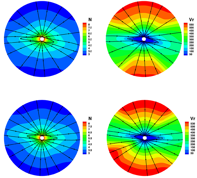
Figure 2. The model results with CT divergence cleaning method, the magnetic field lines, radial speed v_r (km/s), and number density $N(lo{g}_{10}∕{\text{cm}}^3)$ on the meridional plane of ϕ = 180° − 0° (top) and ϕ = 270°−90° (bottom) from 1 to 20 R_s.

FIGURE 3

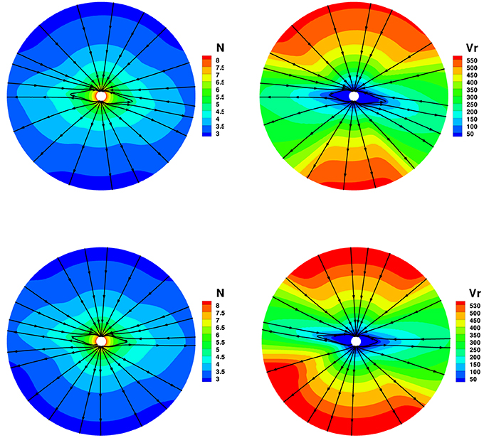
Figure 3. The model results with diffusive divergence cleaning method, the magnetic field lines, radial speed v_r (km/s), and number density $N(lo{g}_{10}∕{\text{cm}}^3)$ on the meridional plane of ϕ = 180° − 0° (top) and ϕ = 270°−90° (bottom) from 1 to 20 R_s.

FIGURE 4

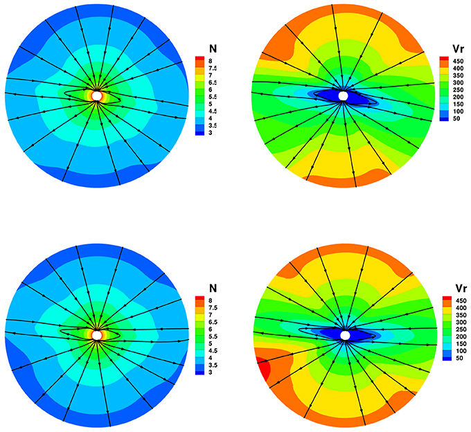
Figure 4. The model results with projection divergence cleaning method, the magnetic field lines, radial speed v_r (km/s), and number density $N(lo{g}_{10}∕{\text{cm}}^3)$ on the meridional plane of ϕ = 180° − 0° (top) and ϕ = 270°−90° (bottom) from 1 to 20 R_s.

FIGURE 5

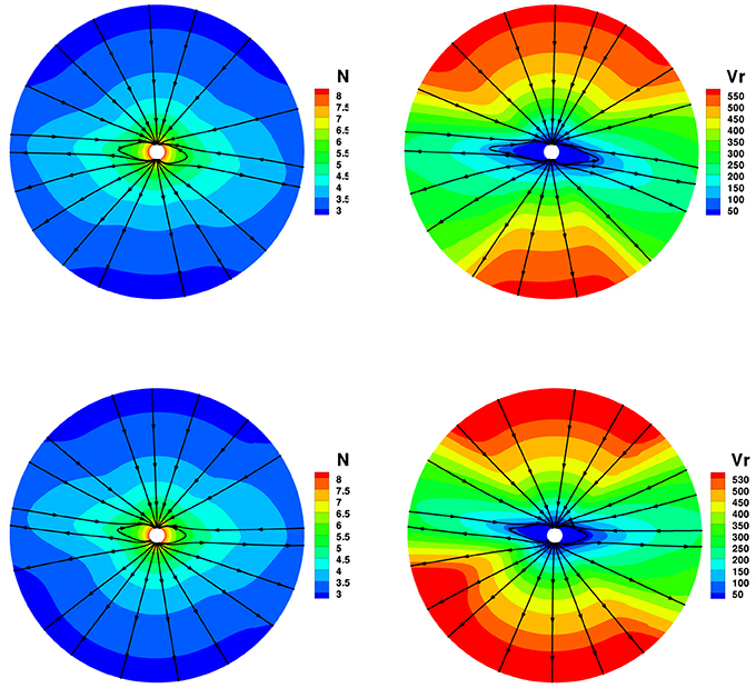
Figure 5. The model results with GLM divergence cleaning method, the magnetic field lines, radial speed v_r (km/s), and number density $N(lo{g}_{10}∕{\text{cm}}^3)$ on the meridional plane of ϕ = 180° − 0° (top) and ϕ = 270°−90° (bottom) from 1 to 20 R_s.

Figure 6 presents the variation of number density N and radial speed v_r from 1 R_s to 20 R_s with the four divergence cleaning methods at different latitudes θ = 174° and θ = 100°, where θ = 174° corresponds to the open field region while θ = 100° corresponds to the HCS region. Reasonably, the speed is larger in the open field region holding the fast solar wind, while the speed is smaller in the HCS region for the slow solar wind, and the number density changes contrarily to that of the speed. Overall, the four divergence cleaning methods can all produce large-scale solar wind.

FIGURE 6

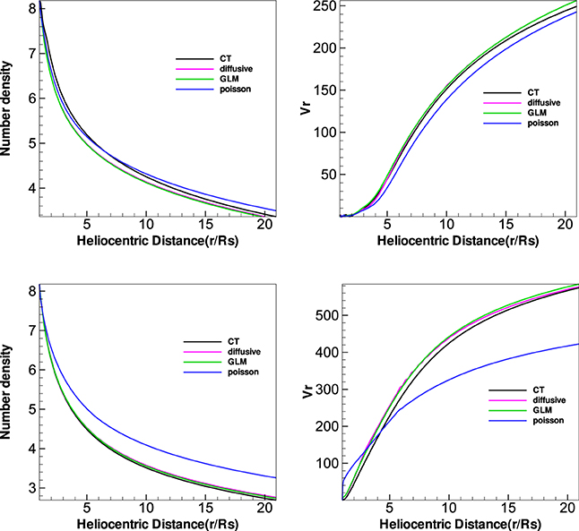
Figure 6. The number density $N({\text{log}}_{10}∕{\text{cm}}^3)$ and radial speed v_r (km/s) distribution along heliocentric distance with different latitudes θ = 100° (top) and θ = 174° (bottom) at the same longitude ϕ = 0° from the four divergence cleaning methods.

To quantitatively see how ∇ · B evolves, we define three relative divergence errors of the cell as $\text{Error}1(\text{B})=\frac{|{\int }_{V_k}\nabla ·\text{B}dV|}{{\int }_{S_k}\left|\text{B}\right|dS}$, Error2(B) = $\frac{|\nabla ·\text{B}|·\left|R\right|}{\left|\text{B}\right|}$, and $\text{Error}3(\text{B})=\frac{|\nabla ·\text{B}|·\left|R\right|}{\sqrt{2p}}$ (Powell et al., 1999; Pakmor and Springel, 2013; Mocz et al., 2014), where V_k is the kth sliding volume cell involved with the mesh grids, and S_k is the surface areas involved with V_k, and $R=\sqrt{\frac{3}{\frac{1}{{(\Delta r)}^2}+\frac{1}{{(r\Delta \theta )}^2}+\frac{1}{{(r sin \theta \Delta \varphi )}^2}}}$ is the characteristic size of the cell. Figures 7–9 show the Error1(B) and Error2(B) and Error3(B) of the four divergence cleaning methods at t = 5 h on the meridional plane of ϕ = 180° − 0°. From these figures we can see that all the divergence cleaning methods can keep the ∇ · B related errors under control, however, there are some differences in the relative magnitude of the resulting divergence errors. As is clearly visible in these figures, the divergence error is larger in the inner boundary for CT method compared to the other three methods, as to the outer region, that is on the contrary. That is because the local divergence error can be convected out of the domain using the diffusive method, the projection method or the GLM method, and the CT method maintain the initial divergence error unchanged in computation.

FIGURE 7

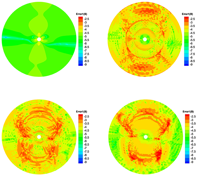
Figure 7. The log₁₀Error1(B) in the calculation at t = 5 h on the meridional plane of ϕ = 180° − 0° from 1 to 20 R_s, the results from CT method (left) and diffusive method (right) are displayed in the top row, the bottom row is from the projection method (left) and GLM method (right).

FIGURE 8

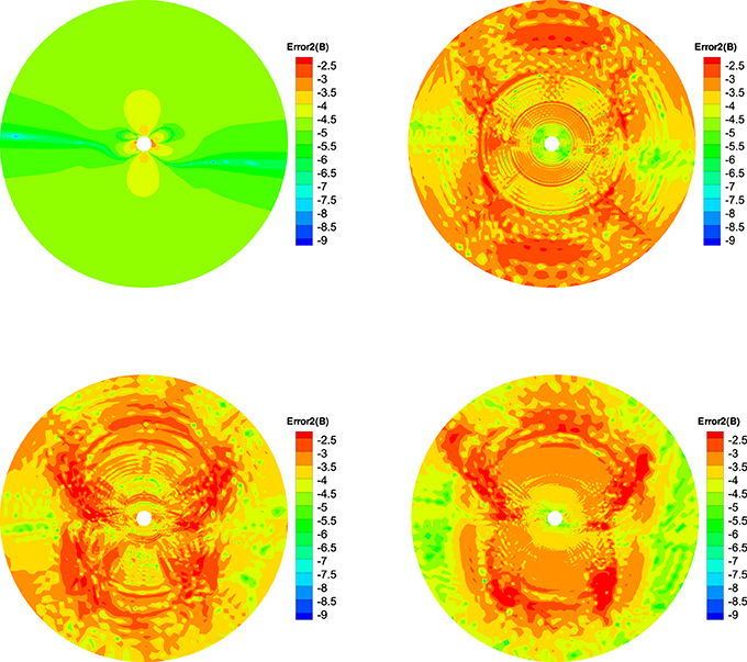
Figure 8. The log₁₀Error2(B) in the calculation at t = 5 h on the meridional plane of ϕ = 180° − 0° from 1 to 20 R_s, the results from CT method (left) and diffusive method (right) are displayed in the top row, the bottom row is obtained from the projection method (left) and GLM method (right).

FIGURE 9

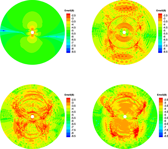
Figure 9. The log₁₀Error3(B) in the calculation at t = 5 h on the meridional plane of ϕ = 180° − 0° from 1 to 20 R_s, the results from CT method (left) and diffusive method (right) are displayed in the top row, the bottom row follows from the projection method (left) and GLM method (right).

Figures 10–12 show the Error1(B), Error2(B), and Error3(B) of the four divergence cleaning methods at t = 20 h on the meridional plane of ϕ = 180° − 0°. Compared to Figures 7–9, there have small difference of the four methods, which verify that these methods keeping the divergence error small and no obvious large error appears in computation. The divergence error for CT method stays almost the same after t = 5 h. As for GLM method, the divergence error is convected out of the domain. Overall, the spatial distribution of the errors for these four methods are very similar and the relative divergence errors are around 10⁻³ − 10⁻⁸.

FIGURE 10

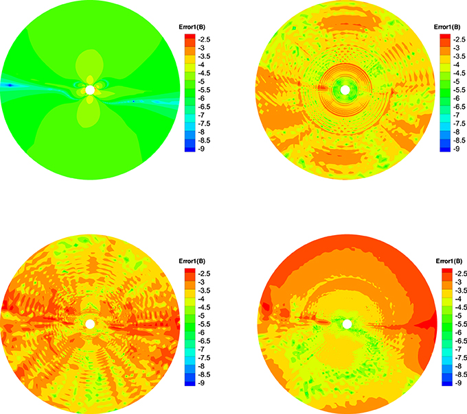
Figure 10. The log₁₀Error1(B) in the calculation at t = 20 h on the meridional plane of ϕ = 180° − 0° from 1 to 20 R_s, the results from CT method (left) and diffusive method (right) are displayed in the top row, the bottom row is provided by the projection method (left) and GLM method (right).

FIGURE 11

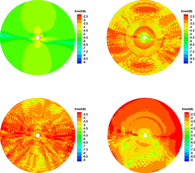
Figure 11. The log₁₀Error2(B) in the calculation at t = 20 h on the meridional plane of ϕ = 180° − 0° from 1 to 20 R_s, the results from CT method (left) and diffusive method (right) are displayed in the top row, the bottom row is produced from the projection method (left) and GLM method (right).

FIGURE 12

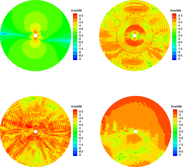
Figure 12. The log₁₀Error3(B) in the calculation at t = 20 h on the meridional plane of ϕ = 180° − 0° from 1 to 20 R_s, the results from CT method (left) and diffusive method (right) are displayed in the top row, the bottom row is produced from the projection method (left) and GLM method (right).

Figure 13 gives the evolution of the average relative divergence errors as a function of time from the four methods in the calculation. The average relative divergence errors defined as Error1(B)^ave = $\sum _{k=1}^M\frac{|{\int }_{V_k}\nabla ·\text{B}dV|}{{\int }_{S_k}\left|\text{B}\right|dS}∕M$, $\text{Error}2{(\text{B})}^{ave}=\sum _{k=1}^M\frac{|\nabla ·\text{B}|·\left|R\right|}{\left|\text{B}\right|}∕M$, $\text{Error}3{(\text{B})}^{ave}=\sum _{k=1}^M\frac{|\nabla ·\text{B}|·\left|R\right|}{\sqrt{2p}}∕M$, where M is the total number of cells in the computational domain. From this figure we can see that Error1(B)^ave for CT method is around 10^−4.6, for diffusive method is around 10^−3.7, for GLM method is around 10^−3.6 and for projection method is around 10^−3.2. The Error2(B)^ave is larger than Error1(B)^ave and Error3(B)^ave. The average relative divergence errors stay the same after 10 h and no obvious large error appears after a long run time. This verifies that the numerical error for the magnetic field divergence can continue to be acceptable during calculation. The CT method has the smallest average relative divergence errors compared to the other three methods and the errors stay the same as initial in calculation, the initial magnetic fields evaluated in the discretized space contributes significantly to the average relative divergence errors. The average relative divergence errors for diffusive method are smaller than GLM method or projection method. The relative divergence errors of diffusive method and projection method are affected by maximal sub-iterations, increasing maximal sub-iterations will make the relative divergence errors decrease but is time-consuming. Figures 14, 15 shows the average relative divergence errors for diffusive method and projection method using maximal sub-iterations 30. The Error1(B)^ave for diffusive method is about 10^−4.3, and for projection method is about 10^−3.3, the errors become small compared to Figure 13. Since increasing the maximal sub-iterations will decrease the computation efficiency, and Figure 13 also shows the results are acceptable without increasing the maximal sub-iterations. So we use sub-iteration 1 for diffusive method and maximal sub-iterations 10 for projection method in our code.

FIGURE 13

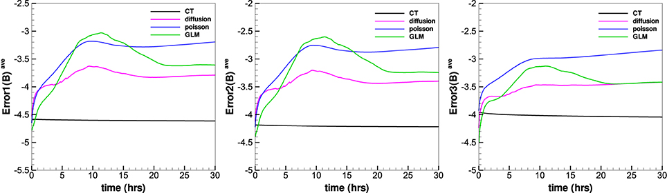
Figure 13. The temporal evolution of the $lo{g}_{10}\text{Error1}{(\text{B})}^{ave}$, $lo{g}_{10}\text{Error2}{(\text{B})}^{ave}$, and $lo{g}_{10}\text{Error3}{(\text{B})}^{ave}$ from the four divergence cleaning methods in the calculation.

FIGURE 14

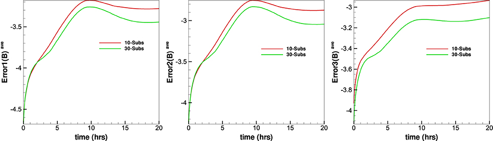
Figure 14. The temporal evolution of the $lo{g}_{10}\text{Error1}{(\text{B})}^{ave}$ and $lo{g}_{10}\text{Error2}{(\text{B})}^{ave}$ and $lo{g}_{10}\text{Error3}{(\text{B})}^{ave}$ from the projection method with different maximal sub-iterations.

FIGURE 15

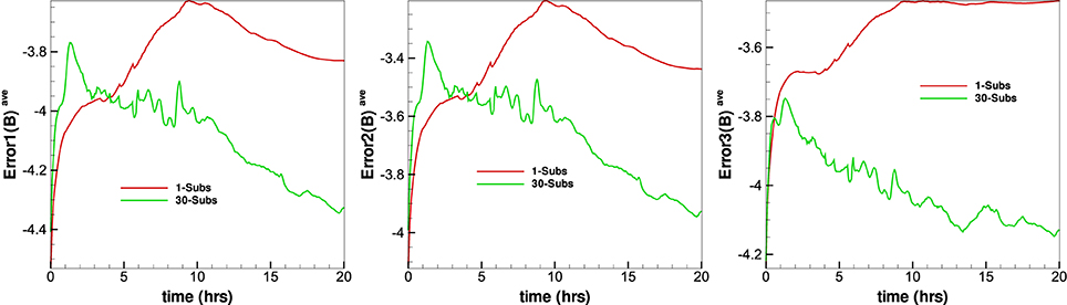
Figure 15. The temporal evolution of the $lo{g}_{10}\text{Error1}{(\text{B})}^{ave}$ and $lo{g}_{10}\text{Error2}{(\text{B})}^{ave}$ and $lo{g}_{10}\text{Error3}{(\text{B})}^{ave}$ from the diffusive method with different maximal sub-iterations.

It is important to note that for all methods the average relative divergence errors are small, the spatial distribution of the errors are very similar for them. Although the employed approach to limit divergence errors are significantly different and there have some differences in the average relative divergence errors as a function of time, there are excellent agreement for them in solar corona simulation, they can all produce structured solar wind.

6. Conclusions and Discussions

In this study, we employ four methods to maintain divergence cleaning constraint of magnetic field and compared the differences between them in solar corona simulation. All these algorithms are combined with a finite-volume scheme based on a six-component grid system in spherical coordinates (Ziegler, 2011, 2012; Feng et al., 2014), numerical results show that they can all produce large-scale solar wind though the relative divergence errors are different for them.

The CT method maintain the ∇ · B = 0 constraint by utilizing a special discretization on a staggered grid. This method evolves area-averaged magnetic field components at the cell faces rather than volume-averaged quantities as fluid part, and electric field components on cell edges are needed. The CT method is attractive from a physical point of view, however, requires the magnetic field variables to be treated differently from the fluid variables, which may be inconvenient for implementation. The diffusive method reduce the numerical error of ∇ · B by adding a source term in the induction equation. The projection method involves the solution of a poisson equation after every time step to correct errors of ∇ · B, and thus can be coupled with any numerical scheme, but solving the additional Poisson equation can significantly increase the computational cost. The GLM method maintain the ∇ · B = 0 constraint by introducing a newly transport variable ψ is to the MHD system. The GLM method is fully conservative in mass, momentum, magnetic induction and energy, it is effective in controlling divergence error and can easily be applied on general grids. Our numerical results showed the CT method can maintain the average relative divergence error around 10^−4.5. The diffusive method can maintain the average relative divergence error about 10^−3.6, and we only use sub-iteration 1 in this paper, increasing maximal sub-iterations will decrease the relative divergence error. The average relative divergence error for GLM method is about 10^−3.3 and for projection method is 10^−3.1. So the CT method and the diffusive approach can maintain divergence cleaning constraint better, the diffusive method is a good choice by considering simplicity, and the CT method should be considered while we want to capture the discontinuity structure. The projection method in our paper is a preliminary try and we think the result can be better if we use multigrid in the future.

Although there have some differences in the average relative divergence errors for the four employed methods, the differences dose't effect the large-scale solar wind structure and they can all produce structured solar wind. They all produce many typical properties of the solar wind, such as an obvious slow speed area near the slightly tilted HCS plane and a fast speed area near the poles, and high density in the slow speed area and vice versa in both poles. Overall, our model can produce all the physical parameters everywhere within the computation domain.

Author Contributions

MZ run the cases and plotted all the figures. Both MZ and XF are involved in the development of the three-dimensional MHD code, the analysis numerical results, the writing of the manuscript.

Conflict of Interest Statement

The authors declare that the research was conducted in the absence of any commercial or financial relationships that could be construed as a potential conflict of interest.

Acknowledgments

The work is jointly supported by the National Basic Research Program of China (Grant No. 2012CB825601), the National Natural Science Foundation of China (Grant Nos. 41231068, 41504132, 41274192, and 41531073), the Knowledge Innovation Program of the Chinese Academy of Sciences (Grant No. KZZD-EW-01-4), and the Specialized Research Fund for State Key Laboratories. The numerical calculation has been completed on our SIGMA Cluster computing system. The Wilcox Solar Observatory is currently supported by NASA.

References

Balsara, D. S., and Kim, J. (2004). A comparison between divergence-cleaning and staggered-mesh formulations for numerical magnetohydrodynamics. Astrophys. J. 602, 1079–1090. doi: 10.1086/381051

CrossRef Full Text | Google Scholar

Brackbill, J. U., and Barnes, D. C. (1980). The effect of nonzero ∇·B on the numerical solution of the magnetohydrodynamic equations. J. Comput. Phys. 35, 426–430. doi: 10.1016/0021-9991(80)90079-0

CrossRef Full Text | Google Scholar

Brandenburg, A., Rädler, K. H., Rheinhardt, M., and Käpyla, P. J. (2008). Magnetic diffusivity tensor and dynamo effects in rotating and shearing turbulence. Astrophys. J. 676, 740–751. doi: 10.1086/527373

CrossRef Full Text | Google Scholar

Dedner, A., Kemm, F., Króner, D., Munz, C. D., Schnitzer, T., and Wesenberg, W. (2002). Hyperbolic divergence cleaning for the MHD equations. J. Comput. Phys. 175, 645–673. doi: 10.1006/jcph.2001.6961

CrossRef Full Text | Google Scholar

Dedner, A., Rohde, C., and Wesenberg, M. (2003). “A new approach to divergence cleaning in magnetohydrodynamic simulations,” in Hyperbolic Problems: Theory, Numerics, Applications, eds T. Y. Hou and E. Tadmor (Berlin; Heidelberg: Spring-Verlag), 509–518. doi: 10.1007/978-3-642-55711-8-47

CrossRef Full Text

Evans, C. R., and Hawley, J. F. (1988). Simulation of magnetohydrodynamic flows-a constrained transport method. Astrophys. J. 332, 659–677. doi: 10.1086/166684

CrossRef Full Text | Google Scholar

Feng, X., Zhang, M., and Zhou, Y. (2014). A new three-dimensional solar wind model in spherical coordinates with a six-component grid. Astrophys. J. Suppl. Ser. 214, 6. doi: 10.1088/0067-0049/214/1/6

CrossRef Full Text | Google Scholar

Feng, X. S., Jiang, C. W., Xiang, C. Q., Zhao, X. P., and Wu, S. T. (2012a). A data-driven model for the global coronal evolution. Astrophys. J. 758, 62. doi: 10.1088/0004-637X/758/1/62

CrossRef Full Text | Google Scholar

Feng, X. S., Yang, L. P., Xiang, C. Q., Jiang, C. W., Ma, X. P., Wu, S. T., et al. (2012b). Validation of the 3D AMR SIP-CESE solar wind model for four Carrington rotations. Solar Phys. 279, 207–229. doi: 10.1007/s11207-012-9969-9

CrossRef Full Text | Google Scholar

Feng, X. S., Yang, L. P., Xiang, C. Q., Liu, Y., Zhao, X. P., and Wu, S. T. (2012c). “Numerical study of the global corona for CR 2055 driven by daily updated synoptic magnetic field,” in Astronomical Society of the Pacific Conference Series, Vol. 459 (San Francisco, CA), 202–208.

Google Scholar

Feng, X. S., Yang, L. P., Xiang, C. Q., Wu, S. T., Zhou, Y. F., and Zhong, D. K. (2010). Three-dimensional solar wind modeling from the Sun to Earth by a SIP-CESE MHD model with a six-component grid. Astrophys. J. 723, 300–319. doi: 10.1088/0004-637X/723/1/300

CrossRef Full Text | Google Scholar

Feng, X. S., Zhang, S. H., Xiang, C. Q., Yang, L. P., Jiang, C. W., and Wu, S. T. (2011). A hybrid solar wind model of the CESE+HLL method with a Yin-Yang overset grid and an AMR grid. Astrophys. J. 734, 50. doi: 10.1088/0004-637X/734/1/50

CrossRef Full Text | Google Scholar

Fuchs, F. G., Mishra, S., and Risebro, N. H. (2009). Splitting based finite volume schemes for ideal MHD equations. J. Comput. Phys. 228, 641–660. doi: 10.1016/j.jcp.2008.09.027

CrossRef Full Text | Google Scholar

Hayashi, K. (2005). Magnetohydrodynamic simulations of the solar corona and solar wind using a boundary treatment to limit solar wind mass flux. Astrophys. J. Suppl. Ser. 161, 480–494. doi: 10.1086/491791

CrossRef Full Text | Google Scholar

Inoue, S., Hayashi, K., Magara, T., Choe, G. S., and Park, Y. D. (2015). Magnetohydrodynamic Simulation of the X2.2 Solar Flare on 2011 February 15. II. Dynamics Connecting the Solar Flare and the Coronal Mass Ejection. Solar Stell. Astrophys. 803, 73. doi: 10.1088/0004-637X/803/2/73

CrossRef Full Text | Google Scholar

Jiang, R. L., Fang, C., and Chen, P. F. (2012a). A new MHD code with adaptive mesh refinement and parallelization for astrophysics. Comput. Phys. Commun. 183, 1617–1633. doi: 10.1016/j.cpc.2012.02.030

CrossRef Full Text | Google Scholar

Jiang, R. L., Fang, C., and Chen, P. F. (2012b). Numerical simulation of solar microflares in a canopy-type magnetic configuration. Astrophys. J. 751, 152. doi: 10.1088/0004-637X/751/2/152

CrossRef Full Text | Google Scholar

Linker, J. A., Mikić, Z., Biesecker, D. A., Forsyth, R. J., Gibson, S. E., Lazarus, A. J., et al. (1999). Magnetohydrodynamic modeling of the solar corona during whole Sun month. J. Geophys. Res. 104, 9809–9830. doi: 10.1029/1998JA900159

CrossRef Full Text | Google Scholar

Manabu, Y., Kanako, S., and Yosuke, M. (2009). Development of a magnetohydrodynamic simulation code satisfying the solenoidal magnetic field condition. Comput. Phys. Commun. 180, 1550–1557. doi: 10.1016/j.cpc.2009.04.010

CrossRef Full Text | Google Scholar

Mignone, A., and Tzeferacos, P. (2010). A second-order unsplit Godunov scheme for cell-centered MHD: the CTU-GLM scheme. J. Comput. Phys. 229, 2117–2138. doi: 10.1016/j.jcp.2009.11.026

CrossRef Full Text | Google Scholar

Mignone, A., Tzeferacos, P., and Bodo, G. (2010). High-order conservative finite difference GLM-MHD schemes for cell-centered MHD. J. Comput. Phys. 229, 5896–5920. doi: 10.1016/j.jcp.2010.04.013

CrossRef Full Text | Google Scholar

Mocz, P., Vogelsberger, M., and Hernquist, L. (2014). A constrained transport scheme for mhd on unstructured static and moving meshes. Month. Notices R. Astron. Soc. 442, 43–55. doi: 10.1093/mnras/stu865

CrossRef Full Text | Google Scholar

Pakmor, R., and Springel, V. (2013). Simulations of magnetic fields in isolated disc galaxies. Month. Notices R. Astron. Soc. 432, 176–193. doi: 10.1093/mnras/stt428

CrossRef Full Text | Google Scholar

Parker, E. N. (1963). Interplanetary Dynamical Processes. New York, NY: Interscience Publishers.

Google Scholar

Powell, K. G., Roe, P. L., Linde, T. J., Gombosi, T. I., and De Zeeuw, D. L. (1999). A solution-adaptive upwind scheme for ideal magnetohydrodynamics. J. Comput. Phys. 154, 284–309. doi: 10.1006/jcph.1999.6299

CrossRef Full Text | Google Scholar

Powell, K. G., Roe, P. L., and Quirk, J. (1993). “Adaptive-mesh algorithms for computational fluid dynamics,” in Algorithmic Trends in Computational Fluid Dynamics, eds M. Y. Hussaini, A. Kumar and M. D. Salas (New York, NY: Springer), 303–337. doi: 10.1007/978-1-4612-2708-3-18

CrossRef Full Text

Rempel, M., Schüssler, M., and Knölker, M. (2009). Radiative magnetohydrodynamic simulation of sunspot structure. Astrophys. J. 691, 640–649. doi: 10.1088/0004-637X/691/1/640

CrossRef Full Text | Google Scholar

Shen, F., Shen, C. L., Zhang, J., Hess, P., Wang, Y. M., Feng, X. S., et al. (2014). Evolution of the 12 July 2012 CME from the sun to the earth: data-constrained three-dimensional MHD simulations. J. Geophys. Res. Space Phys. 119, 7128–7141. doi: 10.1002/2014JA020365

CrossRef Full Text | Google Scholar

Susanto, A., Ivan, L., Sterck, H. D., and Groth, C. P. T. (2013). High-order central ENO finite-volume scheme for ideal MHD. J. Comput. Phys. 250, 141–164. doi: 10.1016/j.jcp.2013.04.040

CrossRef Full Text | Google Scholar

Tóth, G. (2000). The ∇ · B = 0 constraint in shock-capturing magnetohydrodynamics codes. J. Comput. Phys. 161, 605–652. doi: 10.1006/jcph.2000.6519

CrossRef Full Text | Google Scholar

Tóth, G., Sokolov, I. V., Gombosi, T. I., Chesney, D. R., Clauer, C. R., Zeeuw, D. L. D., et al. (2005). Space weather modeling framework: a new tool for the space science community. J. Geophys. Res. 110, A12226. doi: 10.1029/2005JA011126

CrossRef Full Text | Google Scholar

Tóth, G., van der Holst, B., Sokolov, I. V., De Zeeuw, D. L., Gombosi, T. I., Fang, F., et al. (2012). Adaptive numerical algorithms in space weather modeling. J. Comput. Phys. 231, 870–903. doi: 10.1016/j.jcp.2011.02.006

CrossRef Full Text | Google Scholar

van der Holst, B., and Keppens, R. (2007). Hybrid block-AMR in Cartesian and curvilinear coordinates: MHD applications. J. Comput. Phys. 226, 925–946. doi: 10.1016/j.jcp.2007.05.007

CrossRef Full Text | Google Scholar

Yee, K. (1966). Numerical solution of initial boundary value problems involving Maxwell's equations in isotropic media. IEEE Trans. Anten. Propagat. 14, 302–307. doi: 10.1109/TAP.1966.1138693

CrossRef Full Text | Google Scholar

Ziegler, U. (2004). A central-constrained transport scheme for ideal magnetohydrodynamics. J. Comput. Phys. 196, 393–416. doi: 10.1016/j.jcp.2003.11.003

CrossRef Full Text | Google Scholar

Ziegler, U. (2011). A semi-discrete central scheme for magnetohydrodynamics on orthogonal-curvilinear grids. J. Comput. Phys. 230, 1035–1063. doi: 10.1016/j.jcp.2010.10.022

CrossRef Full Text | Google Scholar

Ziegler, U. (2012). Block-structured adaptive mesh refinement on curvilinear-orthogonal grids. SIAM J. Sci. Comput. 34, C102–C121. doi: 10.1137/110843940

CrossRef Full Text | Google Scholar