SE(3) group convolutional neural networks and a study on group convolutions and equivariance for DWI segmentation

We present an SE(3) Group Convolutional Neural Network along with a series of networks with different group actions for segmentation of Diffusion Weighted Imaging data. These networks gradually incorporate group actions that are natural for this type of data, in the form of convolutions that provide equivariant transformations of the data. This knowledge provides a potentially important inductive bias and may alleviate the need for data augmentation strategies. We study the effects of these actions on the performances of the networks by training and validating them using the diffusion data from the Human Connectome project. Unlike previous works that use Fourier-based convolutions, we implement direct convolutions, which are more lightweight. We show how incorporating more actions - using the SE(3) group actions - generally improves the performances of our segmentation while limiting the number of parameters that must be learned.

1 Introduction

In this work, we study the influence of group actions on data and how they may impact the architecture and performances of neural networks, especially convolutional neural networks (CNN). CNNs rely on assumed translational symmetries in data and have shown very robust performance in imaging tasks, especially medical imaging ones, and they are highly parameter-efficient due to their weight-sharing property. When data offer more structure than simply translation, this can be used to build generalized CNNs. This is especially the case for the task at hand—classification and segmentation of Diffusion Weighted Imaging (DWI) data. These Group and Geometric CNNs (GCNN) have been studied intensively and applied in many situations in the few past years (Masci et al., 2015; Cohen and Welling, 2016a; Boscaini et al., 2016; Bekkers et al., 2018; Cohen et al., 2020 to cite a few).

DWI is a non-invasive image modality that provides local information about water diffusion in tissues by means of measuring spin displacement (Tuchs, 2004). It provides three-dimensional diffusion information at each location x that can be encoded as a function f_x on the two-dimensional sphere S². A field of these functions, on a given domain, can be represented as a function f:ℝ³×S² → ℝ. If a sample is rotated and translated, the acquired signal should reflect, up to the limitations of acquisition protocol, this transformation. The group in question is the group of 3D rigid motions, SE(3), and the space ℝ³×S² is a homogeneous space under the action of SE(3): A point in ℝ³×S² can be transformed in any other point by a rigid transformation. This notion of homogeneous space is at the heart of the extension of CNNs to GCNNs (Cohen et al., 2020; Bekkers, 2019).

Our task at hand is the classification/segmentation of diffusion data. The inductive bias provided by the knowledge of these transformations may prove important for our task, especially when the amount of annotated data is limited. The problem boils down to how to incorporate this knowledge. The most classical approach is to use data augmentation, reflecting the expected symmetries in the data, in the hope that the network will be able to learn it during the training phase, learning symmetry-aware kernels.

Incorporating, on the other hand, some information about the symmetries of the data in the model has been shown to boost the performances of these networks (Bekkers et al., 2018). But how much of this information is needed for a given task? To provide an answer, for the DWI segmentation task, we propose several networks, which gradually incorporate these symmetries in their architecture and study their performances. In addition, instead of performing convolution on non-Euclidean data in a spectral fashion using Fourier-type transformations, we implement convolution in all our experiments in a direct way, as is usually done in the image analysis community. In other words, we use regular representations of groups to encode the group actions in the models, instead of irreducible representations. Our experiments, in some sense, perform a group action ablation study. We start with a “naive” CNN and then incorporate spherical symmetries, resulting in a SO(3)-GCNN, discarding the spatial aspect of the data. The spatial aspect is then added in the form of a standard CNN coupled with spherical symmetries, and then, we build a network where roto-translational transformations are used in almost all steps. This work demonstrates empirically the improvement in performance. The results are, however, not always clear-cut. Previous works associated with group convolutions have addressed the capabilities of their models in comparison with data augmentation but, to the best of our knowledge, have not touched the comparison between models tested under randomly transformed test sets. This is what our ablation study is providing. It not only shows the impact of embedding transformations in the model but also gives a systematic analysis on the comparison among different group actions and the corresponding elements of network architecture with respect to the interplay between rotations and translations - the physically justified roto-translation group and the simpler direct product of translations and rotations - imposed in the models, and their relation to data augmentation, both in the training and test set. In the study we provide, the GCNN built from 3D-translations on one hand and rotations, on the other hand, seems to perform better than a SE(3)-GCNN. However, the SE(3)-network generalizes better to unseen rotated data than the previous one. The reason may lie in the particular type of data used - our DWI scans come from the Human Connectome Project (HCP) (Van Essen et al., 2013) are highly preprocessed, including a form of alignment – and this may impact the results. Nevertheless, for every model we propose, we also experiment training them with data augmentation to compare with our equivariant networks. We show that the more equivariance we incorporate into the model, the better the model resists the inconsistency of distributions between training and testing data.

The contribution of this work is as follows.

• We extend the prior work (Liu et al., 2022) with a detailed theoretic formulation of the proposed method. We discretize SO(3) using the icosahedral rotation group and use rotation-translation separable filters in our model to make it very lightweight while achieving highly robust performance.

• We provide an ablation study of different group actions in different spaces and the combinations of these actions with additional experiments using data augmentation.

• We provide a comparison to Müller et al. (2021) in the experiments, which, to our knowledge, is the only other existing work that does tissue classification from DWI data using SE(3) group convolutions. In addition, we further provide experiments using the non-NN method of Schnell et al. (2009), which relies on rotationally invariant spherical harmonic (SH) features extracted from individual DWI voxels (squared-norms at given SH-orders), with classification performed by support vector machines (SVM). The spatial information is, however, discarded.

In the rest of this paper, we review related work, both around CNN and DWI classification problem. Then, we introduce the theoretical setup of GCNN and build several networks. Thereafter, we study and discuss their performances. Our implementation and experiments are publicly available at https://github.com/rliu-p/se3gcnn.

2 Related work

Deep Learning (DL) for non-flat data, or using more complex group actions than just translations, is currently getting more attention from the research field. When it comes to non-flat data, such as the point-wise spherical signals in DWI, particularly relevant related works are the following. A non-rotationally invariant modification was proposed by Boscaini et al. (2016). Schnell et al. (2009) developed an Support Vector Machine (SVM) using rotation-invariant features extracted from Spherical Harmonic decomposition of the HARDI signals, while Skibbe and Reisert (2017) introduced a toolkit for 3D image processing based on Spherical Tensor Algebra (STA), which is particularly well-suited for tasks requiring rotational invariance, such as image enhancement, reconstruction, and feature detection.

The above provide methods for DL-based processing of data on arbitrary manifolds. When the manifold, however, is a homogeneous space, i.e., there is a group action by which any two points on the manifolds can be reached, theory simplifies via a natural generalization of classical convolutions in group convolution neural networks (GCNNs), as was presented in Cohen et al. (2018); Bekkers et al. (2018); and Kondor and Trivedi (2018). GCNNs guarantee global equivariance. However, global equivariance can be complicated and elusive when the underlying geometry is non-trivial, which was discussed in Cohen et al. (2019). An elementary construction on a general manifold is proposed by Schonsheck et al. (2018) via a fixed choice of geodesic paths used to transport filters between points on the manifold, ignoring the effects of path dependency, i.e., holonomy when paths are geodesics. The removal of this path dependency can be obtained by summarizing local responses over local orientations, which is what was done by Masci et al. (2015). To explicitly deal with holonomy, Sommer and Bronstein (2020) proposed a theoretical breakthrough using convolution construction on manifolds based on stochastic processes via the frame bundle.

On the other hand, Cohen et al. (2018) lifted spherical functions to the 3D-rotation group SO(3) and used a generalization of Fourier transform on it to perform convolution. Elaldi et al. (2021) proposed an equivariant spherical deconvolution method to learn the orientation distribution function (ODF). Bouza et al. (2021) generalized convolution to manifold-valued convolutions using Volterra Series, preserving its equivariance. With the generalization of convolution to more complex group actions than translation, several authors (Gens and Domingos, 2014; Cohen and Welling, 2016a; Weiler et al., 2018b,a; Worrall et al., 2017; Kondor and Trivedi, 2018; Bekkers et al., 2018; Andrearczyk et al., 2020; Chakraborty et al., 2018a,b, 2020; Graham et al., 2020) explored the group convolution path for Lie groups and the homogeneous spaces of these groups. Knigge et al. (2022) proposed a separable convolution setup on Lie groups. The relation between group actions, principal bundles and related vector bundles, and convolutional architectures is currently explored (Cohen et al., 2019, 2020; Aronsson, 2022). The latter elucidates important relations between differential geometry of bundles and Reproducible Kernel Hilbert Spaces. Links between partial differential equations, symmetries, and GCNN are studied in Smets et al. (2021). A unifying framework for equivariant DL on manifolds, connecting both the bundle and homogeneous space viewpoint, is given in Weiler et al. (2021) through a notion of coordinate indepencent convolutions.

Most CNNs approach for the processing of DWI signals discards its specific structure. For instance, Golkov et al. (2016) built multi-layer perceptrons in q-space for kurtosis and NODDI mappings. However, the importance of spherical equivariant or invariant structure has been acknowledged for some years now. The importance of the extraction of rotationally invariant features beyond Fractional Anisotropy (Basser et al., 1994) has been recognized in series of DWI works. For instance, Caruyer and Verma (2015) developed invariant polynomials of spherical harmonic (SH) expansion coefficients and discussed their application in population studies. Schwab et al. (2013) proposed a related construction using eigenvalue decomposition of SH operators. Novikov et al. (2018) and Zucchelli et al. (2020) argued their usefulness for understanding microstructures in relation to DWI.

Chakraborty et al. (2018a) proposed a rotation equivariant construction inspired by Cohen et al. (2018) for disease classification. The same authors (Banerjee et al., 2019) used a S²×ℝ⁺ CNN using SHORE function representation for classification in Parkinson's Disease. Sedlar et al. (2020) used a spherical U-Net for f-ODF estimation. The same authors (Sedlar et al., 2021) used a spherical CNN for microstructure parameter estimation, using spherical harmonics representations. Müller et al. (2021) proposed a sixth-D, 3D space and q-space NNs with roto-translation/rotation equivalence properties, targeted at DWI data. Poulenard et al. (2022) reviewed several implementations of SE(3) neural networks and showcased a comparison among these networks. In their work, steerable CNNs generalize better than group CNNs while dealing with inconsistent distributions between training and testing data for 3D images.

While most equivariant methods use spectral representation of groups, we propose an SE(3) network for DWI data that uses regular representation of groups such that the whole model is light-weight, and the implementation for convolution is not only direct but also separable, improving efficiency. A similar idea was used in Chen et al. (2021), for 3D point cloud feature extraction, with, however, important architectural differences due to the nature of input data. Both our method and Chen et al. (2021) implemented regular representations of groups in a separable fashion; however, their separable kernels are only over the spatial and rotation interactions while we additionally split the rotation interactions over 2 axes, making use of the factorization of the icosahedron group into 12 × 5 rotations. We do this to further boost efficiency. Furthermore, Chen et al. (2021) include an attention mechanism in the interaction layers, while instead, we use non-linearities between the separate interaction steps. As our operations are strictly local, including attention mechanism would introduce unnecessary computational overhead, whereas in Chen et al. (2021) the attention mechanism could be critical as a selection mechanism among the global interactions between many points within the point cloud. In addition, we compared our method to Müller et al. (2021) which uses steerable filter bases (spectral representation of groups) for the SE(3) group. In our experiments, in comparison with Müller et al. (2021), we found out, however, that our direct convolution implementation of SE(3) GCNN does not perform inferior to its steerable alternative, and our method is a lot more light-weight.

3 Method

The networks we present will be built from the principle of expanding CNNs to groups and their homogeneous spaces, on which they act by extending convolution operations to functions on groups and their homogeneous spaces. For the rotation group SO(3) and the sphere S² as SO(3)-homogeneous space, the common path for implementing convolutions/correlations is to use irreducible representations (Cohen and Welling, 2016b). This approach can be computationally very intensive, unless one restricts to very low-order irreducible representations, with a resolution trade-off worse than the approximation of SO(3) by the icosahedral rotation group. So we do not follow that path here.

In the next section, we provide the theoretical background for extending convolutions to functions on groups. For the reader's convenience, standard concepts from group theory and group actions that are used to build our new convolution layers are presented in Appendix 1.

3.1 Generalized convolution operations

Classical CNNs use the standard convolution operation on ℝⁿ: for h, κ:ℝⁿ → ℝ, where h is the signal and κ is the kernel, the operation is defined as

$\begin{array}{ll}h*\kappa (\text{x})={\displaystyle {\int }_{{ℝ}^n}}h(\text{y})\kappa (\text{x}-\text{y})d\text{y},\text{x}=(x_1,\dots ,x_n),y=(y_1,\dots y_n).& (1)\end{array}$

Here ℝⁿ is the underlying space of the function, n = 2 for 2D images, and n = 3 for 3D volumetric images. This operation can be extended to vector-valued functions (i.e., functions from ℝⁿ → ℝ^m, they have m channels) and multiple kernels, and this is of course at the heart of the definition of a convolutional layer in a CNN.

Rewrite Equation 1 as

$\begin{array}{ll}h*\kappa (\text{x})={\displaystyle {\int }_{T^n}}h(\text{y})L_{\text{y}}\kappa (\text{x})d\text{y},L_{\text{y}}\kappa :\text{x}\mapsto \kappa (\text{x}-\text{y}).& (2)\end{array}$

L_yκ translates the kernel κ by vector y. This is the left regular representation of 𝕋ⁿ on the space of kernels (see Appendix 1.2.5). Using the regular representation, one gets that the standard convolution (Equation 1) is translation-equivariant, a property generally acknowledged as the main source of success for CNNs:

$\begin{array}{ll}(L_{\text{z}}h)*\kappa (\text{x})=L_{\text{z}}(h*\kappa )(\text{x})=h*\kappa (\text{x}-\text{z}).& (3)\end{array}$

In Appendix 1.2.5, a general definition for the regular representation is given for a Lie group G acting on a homogeneous space ℳ. It is defined by $(L_{g}f)(m)=f(g^{-1}m)$. This is in particular the case when ℳ is a principal homogeneous space of G, and especially when ℳ = G. This leads to a generalization of convolutions for functions defined on a group G: if h, κ:G → ℝ, h*_Gκ, or simply h*κ, if there is no ambiguity, is defined by

$\begin{array}{ll}h*\kappa (g)={\displaystyle {\int }_G}h(u)L_u\kappa (g)du={\displaystyle {\int }_G}h(u)\kappa (u^{-1}g)du.& (4)\end{array}$

Here, du refers to a Haar measure in G (Diestel and Spalsbury, 2014). This operation is equivariant to transformations in the group with respect to the regular representation essentially exactly as in Equation 3:

$\begin{array}{ll}\forall v\in G,(L_{v}h)*\kappa (g)=L_v(h*\kappa )(g)=h*\kappa (v^{-1}g).& (5)\end{array}$

This operation is also equivariant for the left-representation of G.

We deal rarely directly with functions whose domain is a non-trivial group, such as SE(3), or data “indexed” by a non-trivial group. The domain is instead a homogeneous space of the group of interest, such as ℝ³ or the sphere S² for the groups in this work. In that situation, kernel convolution generalizes to a lifting operation that produces a new function, this time defined on the group. If f:ℳ → ℝ and k:ℳ → ℝ are the function and the kernel, respectively, define f*_liftingk, or just f*k, if there is no ambiguity, by

$\begin{array}{ll}f*k(g)={\displaystyle {\int }_{ℳ}}f(m)k(g^{-1}m)dm={\displaystyle {\int }_{ℳ}}f(m)L_g\kappa (m)dm.& (6)\end{array}$

and this convolution operation is equivariant with respect to actions in G:

$\begin{array}{ll}\forall v\in G,(L_{v}f)*k(g)=L_v(f*k)(g)=f*k(h^{-1}g).& (7)\end{array}$

A bit of caution here, as the first regular representation acts on a function f:ℳ → ℝ while the second acts on the function f:G → ℝ. Once the function is lifted onto this group G, group convolutions on G can be performed on the lifted signals as in Equation 4,

The group convolutions and lifting can be stacked in layers like a standard CNN, and this stacking preserves equivariance, producing equivariant layers. Features at the last group convolution layer can be projected back onto the original space of the function by summarizing feature responses over the group. It is similar to max-pooling-like operations in a standard CNN. This type of operation will provide invariance.

Therefore, a roadmap for group convolutions can be summarized as follows:

• Lifting the function signals to the desired group.

• Group convolutions on the lifted signals.

• Projecting the signals back onto the original space.

We formulate these operations in the following sections.

3.1.1 Lifting layer

A function $f:ℳ\to {ℝ}^{N_0}$ can be lifted to the group G via a kernel $\kappa :ℳ\to {ℝ}^{N_1}$ by

$\begin{array}{ll}f*\kappa (g)={\left({\displaystyle \sum _{j=1}^{N_0}}{\displaystyle {\int }_{ℳ}}{f}_j(m){\kappa }_i(g^{-1}m)dm\right)}_{i=1}^{N_1}& (8)\end{array}$

This is a direct extension of Equation 6 to vector-valued functions f. N₀ is the number of input channels, and N₁ the number of output channels. In practice, in this work, the input function is scalar-valued, i.e., N₀ = 1.

3.1.2 Group convolution layer

A feature function $F:G\to {ℝ}^{N_l}$ is transformed by a convolution kernel $K:G\to {ℝ}^{N_{l+1}}$ by

$\begin{array}{ll}F*K(g)={\left({\displaystyle \sum _{j=1}^{N_l}}{\displaystyle {\int }_G}{F}_j(h)K_i(h^{-1}g)dh\right)}_{i=1}^{N_{l+1}}.& (9)\end{array}$

Here N_l is the number of channels from the output of the last layer (equivalent to the number of input channels for the current layer), and N_l+1 is the number of output channels for the current layer.

3.1.3 Projection layer

If needed, feature map F:G → ℝⁿ can be projected to a function f:ℳ → ℝⁿ by summarizing on the fibers (see appendix 1.2.3.)

$\begin{array}{ll}\overline{F}(m)={\displaystyle \underset{h\in G_{m_0}}{max}}F(gh),\text{for any }g\text{ with }g.m_0=m,& (10)\end{array}$

where the max is computed component-wise. This operation is equivariant: $\overline{L_{k}F}=L_k\overline{F}$.

3.1.4 Activation functions and separable kernels

A point-wise activation function α, such as ReLU, is trivially equivariant L_g(αf) = α(L_gf). On manifolds with an underlying product structure, ℳ = ℳ₁×ℳ₂ - this includes homogeneous spaces and groups - one can choose separable kernels κ = κ_ℳ1⊗κ_ℳ2, and activation functions can be intertwined in between Equations 8, 9. For instance, lifting Equation 8 can be replaced by

$\begin{array}{r}f{*}^{\alpha }\kappa (g)={\displaystyle \sum _{i=1}^K}{\displaystyle {\int }_{{ℳ}_1}}\\ \alpha \left({\displaystyle {\int }_{{ℳ}_2}}f(m_1,m_2){\kappa }_2(g^{-1}{m}_2)d{m}_2\right){\kappa }_1(g^{-1}{m}_1)d{m}_1,& (11)\end{array}$

where *^ακ is a shortcut notation for the intertwining of the kernel and activation function. It is easily seen that it preserves equivariance. Having separable kernels increases the efficiency of the model since it increases weight sharing. For example, instead of having kernels defined in ℝ³×S², we have kernels defined in ℝ³ and in S². In this way, all voxels in ℝ³ share the same spherical kernels. This is used in this work.

The spaces used in this work are ℝ³, the sphere S², and the product space ℝ³×S². The groups that we consider are the group of translations of ℝ³, 𝕋³ ≃ ℝ³, the group SO(3) or 3D rotations, the direct product 𝒢 = 𝕋³ × SO(3), and the special Euclidean group SE(3) = SO(3)⋉𝕋³. Note that though 𝒢 and SE(3) are isomorphic as manifolds, they are not as groups: in 𝒢, $(\overrightarrow{t},R).(\overrightarrow{s},S)=(\overrightarrow{t}+\overrightarrow{s},RS)$ while in SE(3), $(R,\overrightarrow{t}).(S,\overrightarrow{s})=(RS,\overrightarrow{t}+R\overrightarrow{s})$. This is also reflected in their respective actions in Table 1, which shows the different combinations of spaces and groups. We refer the readers to Gerken et al. (2023) for more detailed theoretical foundation.

Table 1

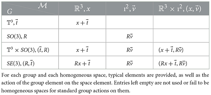
Table 1. Groups and homogeneous spaces in this work.

3.2 Discretization of spherical signals

The way spherical signals are numerically handled have major implications for our networks. A DWI signal is treated as a discretization of a signal f:ℝ³×S² → ℝ. DWIs are acquired, for each voxel, at N fixed directions p₁, …, p_N on S² (here N = 90). These are represented in two different ways.

• Type 1. Ignoring the spherical structure, at each voxel x, we get a measurement vector

$f(x)=(f(x,p_1)\dots ,f(x,p_N))\in {ℝ}^N$. Thus an image is a mapping I:ℝ³ → ℝ^N.

• Type 2. A signal at voxel x is interpolated as a proper spherical function $f(x,\overrightarrow{v})=W(v;v_1,\dots ,v_N)$ where W is a Watson kernel (Jupp and Mardia, 1989). An image from this type is a mapping I:ℝ³×S² → ℝ.

3.3 Direct convolution and discretization of groups

Unlike existing methods that use generalized Fourier-type transforms to perform convolution on spheres (Cohen et al., 2018; Gens and Domingos, 2014; Cohen and Welling, 2016a; Weiler et al., 2018a; Worrall et al., 2017; Kondor and Trivedi, 2018; Bekkers et al., 2018; Andrearczyk et al., 2020; Chakraborty et al., 2018a,b, 2020), we implement the convolution for spheres directly as in classical 2D CNNs in the image analysis field. We first discretize the sphere S² using an icosahedron. To lift the function from the sphere to the SO(3) group, we define a star-shaped kernel k:S²↦ℝ with a limited support. The kernel then moves around the discretized sphere and convolves with signals at each vertex of the icosahedron. It rotates five times at each icosahedral vertex according to the fives edges each vertex has, and collects convolutional responses from all five rotations. In this way, the spherical function is lifted to SO(3), which is discretized by I_SO(3)—the 60 rotational symmetries of an icosahedron. This corresponds to Equation 8 and is shown in Figure 1A. For the SO(3) group convolution layer, the kernel is defined on SO(3), which is represented by the icosahedral symmetries. Here, we specially design the kernel in the way that the support of it covers exactly a fiber. Therefore, we rotate (permute) the kernel at each fiber, convolve the rotated kernels with the fiber, and move the kernel to the next fiber. This is how Equation 9 is implemented, and more details can be found in Figure 1B. With the impact of discretization of the groups and the interpolation of signals, we lose the benefits of learning from raw data. However, the experiments show that the 60 icosahedral symmetries can approximate the SO(3) group well enough such that the models can deal with rotational variations in the data that are different from the rotations used in the discretization.

Figure 1

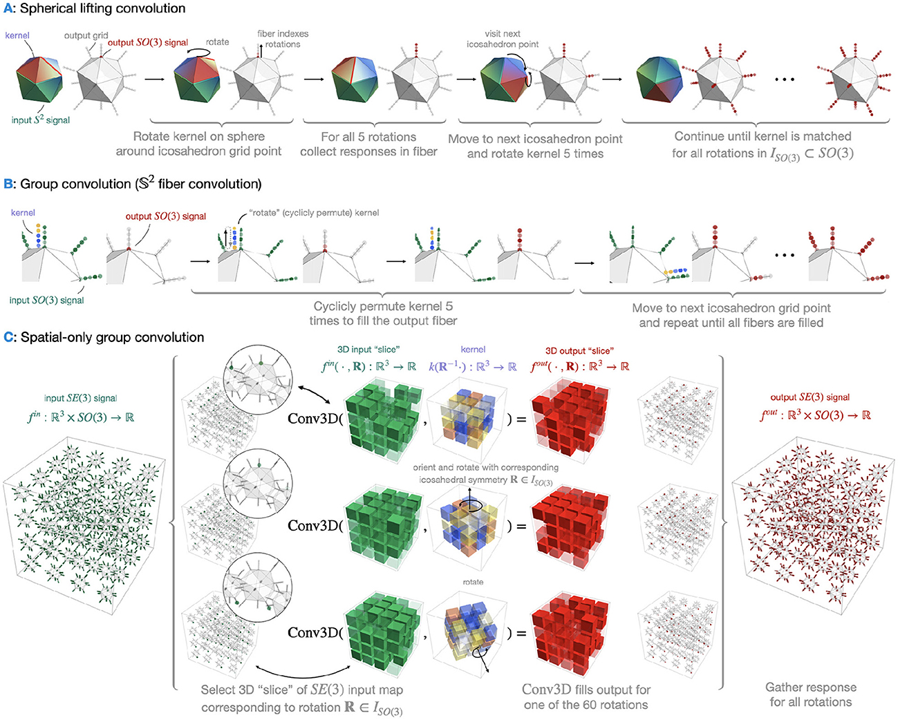
Figure 1. Three group convolution operators used in this paper. (A) shows the spherical part of the separable lifting convolution. The star-shaped kernel translates (in this case translation is equivalent to rotation) to the 12 icosahedron vertices like a spider crawling on a sphere. At each vertex location, the kernel rotates five times aligned with the edges of the icosahedron and gets five responses from all the orientations. Therefore, at each vertex, the output is a fiber consisting of five elements. There are in total 60 responses from all 12 vertices, and thus 60 rotation matrices to translate the kernel, assembling a discretization of SO(3) - I_SO(3). (B) shows the spherical part of the separable group convolution. The kernel is then defined at each fiber and is rotated (permuted) again for five times to get the responses of different orientations, as in the lifting convolution. (C) shows the spatial part of the separable convolution (the spatial convolution is the same in the lifting and group convolution; thus, we only show one). The spatial kernel is a 3D grid. The grid is rotated to convolve with all 60 spherical responses. The kernel is rotated 60 times, using the same icosahedral symmetry rotations as those on which the input is sampled.

3.4 Generic networks used in this work

We present four constructions in which gradual levels of complexity in group actions are introduced. This can be seen as a group action ablation study. The precise description of each network will be provided in Section 4.

3.4.1 Group of translations 𝕋³

The S²-structure of the signal is ignored, using the Type 1 discretization. The group being 𝕋³, just another name for ℝ³, we just obtain a standard CNN, ignoring rotational information. An illustration can be found in Figure 2.

Figure 2

Figure 2. Illustration of the classical CNN. In the grids shown above, which assembles the dimensions of feature maps in the later experiments. Each voxel in the ith layer contains C_i values, indicating the numbers of channels. C₁ here is the number of signal values each voxel from the original scan, thus 90. Due to striding, the grid shrinks to 1 voxel after 3 convolutional layers and then is fed into a fully connected layer for classification.

3.4.2 SO(3)

This time the spatial structure is ignored, and each voxel provides a spherical data point. Type 2 discretization is used. The GCNN takes as input a spherical function and will classify it by performing SO(3)-lifting, SO(3)-convolutions and summarization. The convolved function on SO(3) is then projected back to S² by this summarization. It is illustrated in Figures 1A, B. This model is a fully equivariant implementation of SO(3) group convolution followed by the work in Liu et al. (2021), which does not hold global equivariance.

3.4.3 𝕋³ × SO(3)

Spatial and spherical structures are decoupled. This implies a standard spatial CNN dealing with only voxel translations, and a SO(3)-GCNN part for the directional signal. Type 2 discretization is used for spherical signals. The decoupled ℝ³-layer and S²-layer are with group actions 𝕋³ and SO(3), respectively. The illustration for the S²-layer can be found in Figures 1A, B, and the illustration for the ℝ³-layer can be regarded as only one Conv3D operation in Figure 1C without the rotations. Note that since the spatial convolution does not incorporate rotational equivariance, it does not reflect equivariance of the DWI measurements. I.e., one can expect that when the brain rotates, the spatial patterns rotate, as well as their spherical diffusion signals. This model takes rotation into account in the spherical part of the signal but not the spatial part. The projection at the end collapses the function in the group back to ℝ³ by summarizing—in this case, maximizing—over SO(3), and the resulting feature map is fed into a fully connected layer to perform the classification task.

3.4.4 SE(3)

Type 2 discretization is used, and the network uses the full interplay between spatial roto-translations and corresponding rotations of the spherical signal and is thus fully equivariant to SE(3) transformations on the DWI data. Figures 1A, B shows the kernels of the S²-layer. When the kernel moves from one vertex to another, it follows a specific rotation that maps the one-ring neighborhood of the source vertex to the one-ring neighborhood of the target vertex. At each vertex, the kernel has an SO(2) symmetry group structure discretized by 5 rotations. Figure 1C shows the kernel for the ℝ³-layer. It is rotated with the same rotation matrices that moved the S²-kernel as in Figures 1A, B. Since the spatial kernels are cube-shaped grids, interpolation is required while rotating them. Here, we use linear interpolation, which can be easily implemented. To perform the segmentation task, the projection layer collapses the function on SE(3) back to ℝ³ by summarizing—again, maximizing—over SO(3).

4 Experiments and results

In this section, we first list all the detailed network setups, after which we present the results of the experiments. We evaluate our method on the DWI brain dataset from the human connectome project (HCP) (Van Essen et al., 2013). We classify the human brains into four regions - cerebrospinal fluid (CSF), subcortical, white matter (WM), and gray matter (GM). An illustration of the task can be found in Figure 3.

Figure 3

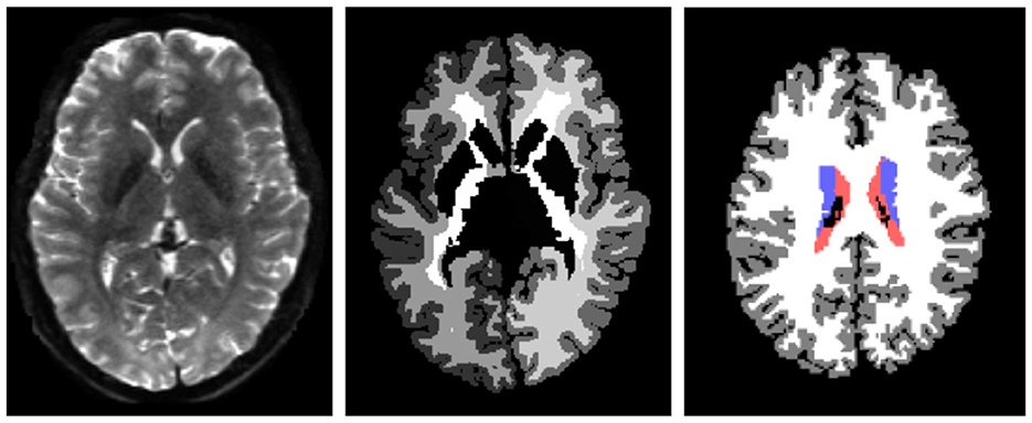
Figure 3. Left to right: original diffusion data, the ground truth segmentation, and the processed ground-truth that we are going to learn from. The label colors for CSF, subcortical, white matter, and gray matter are red, blue, white, and gray, respectively. The figures only illustrate the data, and they are not necessarily from the same slice of the same scan.

We use the preprocessed DWI data (Van Essen et al., 2013) and normalize each DWI scan for the b-1000 images with the voxel-wise average of the b₀. We use the brain masks provided in the dataset to obtain the voxels of interest, while background is ignored. The labels provided with the T1-image are transformed to the DWI using nearest neighbor interpolation (Figure 3). The resolution of the DWI images is 145 × 174 × 145, and the resolution of the T1-images is 260 × 311 × 260. Focal Loss (Lin et al., 2018) is used to counter the class imbalance of the four brain regions. For Focal Loss, all experiments use γ = 2 and use α = (0.35, 0.35, 0.15, 0.15) for CSF, subcortical, WM, and GM, respectively. For the Watson Kernel, all experiments that used this interpolation (Type 2 discretization) have κ = 10. Batch size for all experiments is 100, and the learning rate for all experiments is 0.001.

4.1 Experimental setup

Since each DWI scan is highly resoluted, it is not feasible to use a whole image as input to the networks. Therefore, to reduce the computational burden, as inputting a full DWI volume is intractable, we use spatial windows of N³ voxels, with N = 1 for the SO(3)-action network and N = 7 for the rest. In addition, due to the effect of striding in spatial convolution, the 7³ grid of voxels shrinks to 1³ after 3 spatial convolutions. Therefore, a separable convolution layer (for both 𝕋³ × SO(3) and SE(3) actions) is equivalent to a single SO(3) convolution layer when the grid shrinks to 1³ since the spatial convolution becomes trivial. S² is discretized by a regular icosahedron. SO(3) is discretized as the icosahedral rotation group with 60 elements. Each vertex of the icosahedron is fixed by five rotations, isomorphic to the subgroup of SO(2) consisting of rotations of angle 2kπ/5, k = 0…4. This is, of course, the discretization used for SO(2).

To validate the proposed SE(3) network, we first provide an ablation study of our proposed four types of networks based on different group actions. Then, we compare it with Müller et al. (2021), which implements an SE(3)-GCNN using irreducible representations.

For the ablation study, based on the networks that were introduced above and in alignment with the networks presented in Liu et al. (2022), we design our experiments for them. For each experiment, in order to explore the impact of model capacity on the performance, we construct two models with high and low capacities, respectively, denoted by the superscription + and -. We choose the architectures for the models with low capacity by trying out different complexities and depths and picking the one with the lowest capacity with the same level of performance. Then for the models with high capacity, we simply increase the numbers of kernels in each layer of the models with low capacity.

Detailed descriptions of all the experiments are reported below, and a summary of the experiments can be found in Table 2.

Table 2

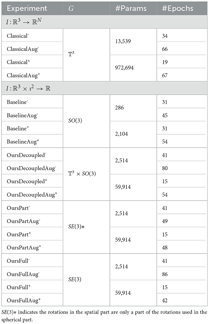
Table 2. Criteria and properties of experiments.

4.2 Ablation study

4.2.1 𝕋³-Classical CNN

The architecture we use is ReLU(ℝ³ conv)−ReLU(ℝ³conv)−ReLU(ℝ³conv)−FC with network setups of a low capacity and a high capacity. FC here is a fully connected layer. We label the small network (90 − 5−5 − 5−4) Classical^- and the big network (90 − 120 − 120 − 90 − 4) Classical⁺.

4.2.2 SO(3)-Baseline

In the experiments, we use the ReLU(lift) −ReLU(gconv)−project−FC architecture as was used in Liu et al. (2021) but with true SO(3)-convolution. The projection layer takes the maximum of the five rotations to collapse the function back to the sphere. We experimented various sizes of the network (10 − 20−proj.−4 and 20 − 40−proj.−4), in addition to the setup used in Liu et al. (2021) (1 − 5−proj.−4). The network that has the biggest size did not seem to improve the second biggest one; thus, we omit it in this paper. Based on the size of the experiments, we call the small network Baseline^- and the big network Baseline⁺.

4.2.3 𝕋³ × SO(3)-OursDecoupled

We use the architecture ReLU(lift)−ReLU(gconv)−ReLU(gconv)−ReLU(gconv) −project−FC. Using separability discussed in Section 3.1.4, a convolution layer (including lifting) is split into two, and ReLU activation is added between separable layers as well. An illustration of the architecture can be found in Figure 4.

Figure 4

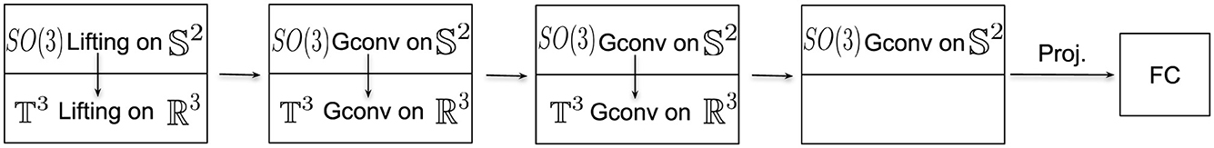
Figure 4. Architecture of the network with group action 𝕋³ × SO(3). Each block is a convolutional layer split into two separable layers. The vertical arrows in each block show the separable convolutions. First, the spherical convolution is applied, followed by the spatial convolution. The last block before the FC layer is equivalent to a single S²-layer as explained in Section 4.1. Illustrations of ReLU actions are omitted for visualization simplicity.

We again experiment with two sizes of the network - a small one and a big one. The small network has 5 − 5−5 − 5−5 − 5−5−proj.−4 kernels for each layer, while the big network has 10 − 20 − 20 − 40 − 40 − 20 − 10−proj.−4. We label them OursDecoupled^- and OursDecoupled⁺.

4.2.4 SE(3)-ours

Here too we use the separable setup described in Section 3.1.4. Thus, a layer is again split into two layers - an S²-layer and an ℝ³-layer, both for lifting and group convolution. The S²-layer is defined as shown in Figures 1A, B. We rotate the ℝ³ kernels and the S² kernels using the same actions. The rotational actions of the kernels can be represented by 60 rotation matrices and is equivalent to the discretization of the SO(3) rotation group using the icosahedral symmetry group, as shown in Figure 1C. As in Section 4.2.3, we use the ReLU(lift)−ReLU(gconv) −ReLU(gconv)−ReLU(gconv)−project−FC architecture. After the separation of the layers, the illustration is showcased in Figure 5. As in Section 4.2.3, ReLU activations are added between separable layers as well.

Figure 5

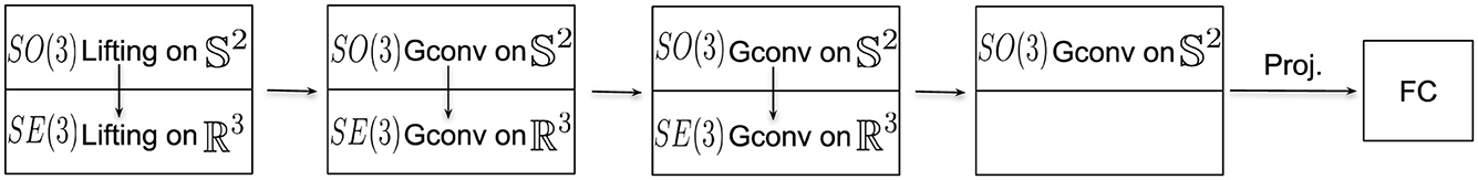
Figure 5. Architecture of the network with group action SE(3).

In addition, we intend to explore the impact of the equivariance we imposed in ℝ³ in this section. As was explained above, we align the rotations of the ℝ³ kernel with the ways the S² kernel moved on the sphere, which is discretized by the 60 rotation symmetries of an icosahedron. At a vertex x_i, i∈1, …, 12 of an icosahedron, there exists a stabilizer SO(3)_xi discretized by 5 equally divided rotations that keep x_i unchanged. Therefore, we also experiment a partial equivariance in the ℝ³ roto-translational convolution. This means at each vertex x_i of the icosahedron, we only take 1 out of the 5 rotations that discretized SO(3)_xi instead of using all of them to rotate the spatial kernel. Note that the partially equivariant models are only fully SE(3)-equivariant when the kernels have a subgroup SO(2) symmetry in them (Bekkers, 2019; Thm 1), which we do not impose and thus equivariance is not guaranteed.

Again, we experiment with two sizes of the network with 5 − 5−5 − 5−5 − 5−5−proj.−4 and 10 − 20 − 20 − 40 − 40 − 20 − 10−proj.−4 kernels, respectively. Therefore, we generate four experiments for this section: OursFull^-, OursPart^-, OursFull⁺, and OursPart⁺.

4.2.5 Data augmentation experiments

To validate the robustness of GCNNs against data variation modeled by group actions, we train all the proposed models with augmented data as well. Each data sample (grid of 7³ or 1³) is randomly rotated on the fly before being fed into the model. To prevent interpolation, the rotations used to transform the data are sampled from a octohedral symmetry group. For DWI data that have directional signals in each voxel, the directions of the signals (b-vectors) in each voxel rotate with the voxel grid. In order to guarantee the signal values in each voxel are from the same orientations after augmentation, we interpolate the function values at the orientations-of-interest using the rotated b-vectors. Therefore, for Type 1 discretization, we interpolate function values at the original b-vectors, and for Type 2 discretization, we interpolate at the pre-defined icosahedron as demonstrated above.

4.3 Results

As was done in Liu et al. (2021), we trained all networks using 1 scan, validated using 1 scan, and tested using 50 scans. We evaluate the accuracies and Dice scores of the classification of the four regions, respectively, and the overall classification accuracy across all test scans. We have also tried training models with more scans (5 or 10); it does not seem to improve the results significantly. Therefore, we choose to use 1 scan for training. For each class, the accuracy is calculated by $\frac{\#CorrectPredictions}{\#ClassSamples}$, and the Dice score is calculated by $\frac{2TP}{2TP+FP+FN}$ for the class. The overall accuracy is calculated by $\frac{\#CorrectPredictions}{\#AllSamples}$.

We trained all models until they converge and before overfitting; thus, models of different capacities and different setups are stopped at different epochs. Each model is trained with both original data and augmented data. Details can be found in Table 2.

The Dice scores and accuracies of models of low capacity can be found in Tables 3, 4, while the Dice scores and accuracies of models of high capacity can be found in Tables 5, 6. The numbers shown in all the tables are the average value and standard deviation across 50 test scans. Examples of predictions compared with the ground truth can be found in Figure 6A.

Table 3

Table 3. Statistics of dice scores from experiments using models of low capacity.

Table 4

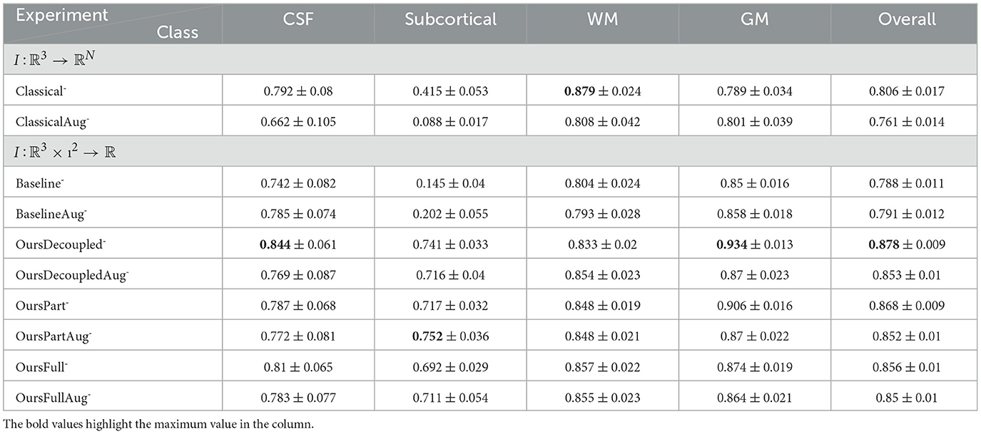
Table 4. Statistics of classification accuracy from all experiments using models of low capacity.

Table 5

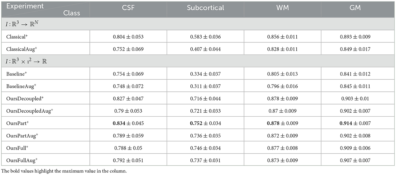
Table 5. Statistics of dice scores from experiments using models of high capacity.

Table 6

Table 6. Statistics of classification accuracy from all experiments using models of high capacity.

Figure 6

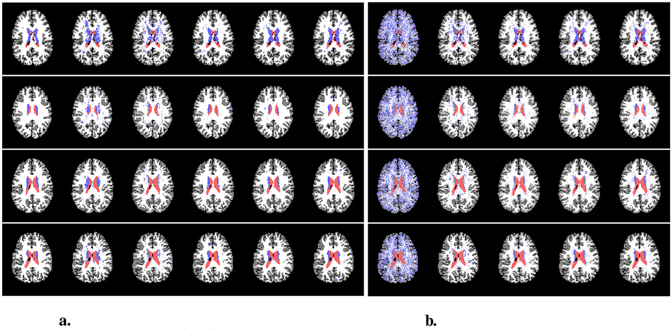
Figure 6. Examples of predictions. (A) shows the predictions from the original test set, and (B) shows the predictions from the augmented (rotated) test set. In (A), from left to right are ground-truth, Classical⁺, Baseline⁺, OursDecoupled⁺, OursPart⁺, and OursFull⁺. In (B), from left to right are Classical⁺, Baseline⁺, OursDecoupled⁺, OursPart⁺, and OursFull⁺. The colors of CSF, subcortical, WM, and GM are red, blue, white, and gray, respectively. (A) Predictions using original data. (B) Predictions using rotated data.

4.3.1 The impact of data augmentation

As we can see from the Tables 3–6, models trained with augmented data do not perform better than their counterparts trained with just original data, if not worse. Unlike 2D image datasets in the computer vision community that have various backgrounds and objects in their images, the HCP dataset is very uniform; thus, the distribution of the original training data is expected to be the same as the test set data. However, after augmentation, the distribution of the training data changed and it differs from the test data. Therefore, in this case, data augmentation does not help any of the models since the augmentation does not represent the diversity in this dataset. One extreme would be Classical^- vs. ClassicalAug^- that can be found in Tables 3, 4, the augmented data confused the model in terms of the subcortical region - a somewhat mixture of white and gray matter which is challenging for models to distinguish. Therefore, from now on, if not specified, we mainly discuss the models and results trained without data augmentation.

4.3.2 The impact of the ℝ³ spatial component

It is easy to observe that the the Baseline experiments perform worst among all. This is an anticipated outcome since it is usually the case that neighboring information is an essential type of local features.

4.3.3 Type 1 discretization vs Type 2 discretization

The classical CNNs use Type 1 discretization, while Type 2 discretization is used for the rest of the models. The classical CNNs do not perform as well as models that take into account the spherical geometry with spatial information but performs better than Baseline. However, Classical^- is not much better than Baseline⁺ while having far more parameters to train, and Classical⁺ performs even worse than OursDecoupled^-, OursPart^-, or OursFull^-, which have much less training parameters.

The results of the two extreme cases—Baseline that only takes into account spherical geometry but ignore any spatial information and Classical that only looks into the spatial part and discards spherical geometry—show that the voxel geometry and neighboring voxel correlation can both capture some decent amount of information to deal with the segmentation task, but they both have something that the other one cannot grasp, and combining the spherical geometry and the spatial correlation can boost the performance to a promising extent.

4.3.4 The impact of adding an ℝ³ part to baseline

On top of the Baseline, the easiest way to add spatial information to the purely voxel-based framework is what was done in OursDecoupled Section 4.2.3—a GCNN on S² to learn the geometric signals in individual signals and a regular classical CNN to take into account the local spatial information. We can see from the results that this setup immediately boosted the performance compared to the Baseline. We can also see that OursDecoupled⁺ performs better than OursDecoupled^-, for the sake of model capacity.

4.3.5 The argument for OursFull not performing the best

For models of low capacity, however, we can observe from Tables 3, 4 that our proposed method performs worse than OursDecoupled^-. In addition, for models of high capacity, even though we can see that OursFull⁺ and OursPart⁺ improve from their low capacity counterparts more than OursDecoupled⁺, OursFull⁺ does not perform as well as OursPart⁺ as shown in Tables 5, 6. This differs from our expectation since models with full roto-translational equivariance should be more capable of handling variances in data, thus should have better performance. Recall that the HCP dataset (Van Essen et al., 2013) contains scans that are preprocessed and aligned with axes, thus there is little variance in rotation. In this case, enforcing SE(3) equivariance in the model can be futile and be even confusing for the model.

To verify this theory, we evaluated all models on the rotated test set. Taking the N³ (N = 1 for Baseline models and N = 7 for the rest) grids of voxels we extracted from the test scans, we randomly rotate each grid using a rotation sampled from the octahedral symmetry group to create a new rotated test set. In this way, we do not need to interpolate while rotating, and the rotations are not aligned with the ones we used in our models to rotate the kernels while still resemble a discretization of the SO(3) group. Hence, we have two categories of models as well as two categories of the test set: models trained with original data vs. models trained with augmented data, and original test set vs. the randomly rotated test set.

4.3.6 Models trained with data augmentation tested with rotated test set

We see that all models trained with augmented training set have very similar performance results to the same models tested with the original test set, and they all perform better in this task than their counterparts trained with the original training set. This checks with our statement in Section 4.3.1 that the consistency of data distributions of the training and test sets boosts test performance. In this case, we used the same kind of rotations while augmenting the training set and test set; therefore, the consistency of data distributions is maintained. However, this can never be guaranteed in real life. We can see this from Tables 7–10.

Table 7

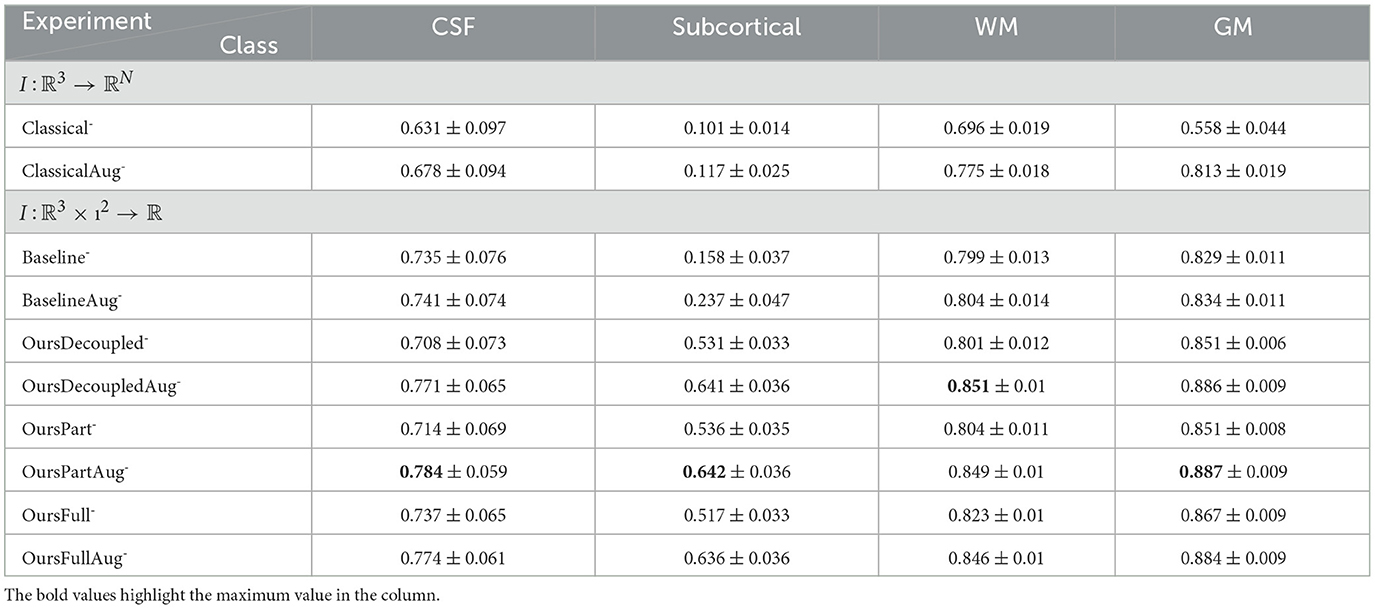
Table 7. Statistics of dice scores from experiments using rotated data and models of low capacity.

4.3.7 Models trained with original data tested with rotated test set

In this section, only models trained without data augmentation are compared and discussed. For models with both low and high capacity, OursFull models have the best performance among other models. OursFull^- remains 0.823 accuracy, decreased from 0.856 while OursFull⁺ decreased from 0.883 to 0.84. This is illustrated in Tables 8, 10. In terms of Dice scores, OursFull^- performs the best for all classes but the subcortical class, and OursFull⁺ has the best results for all classes, as shown in Tables 7, 9.

Table 8

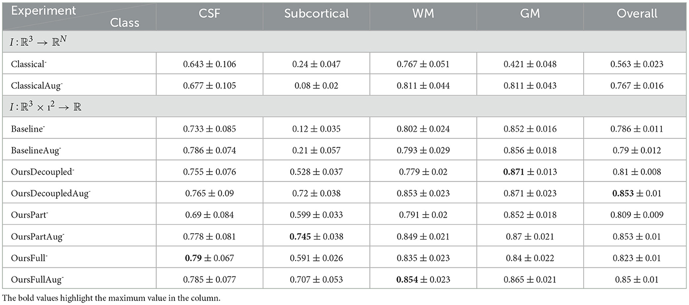
Table 8. Statistics of classification accuracy from experiments using rotated data and models of low capacity.

Table 9

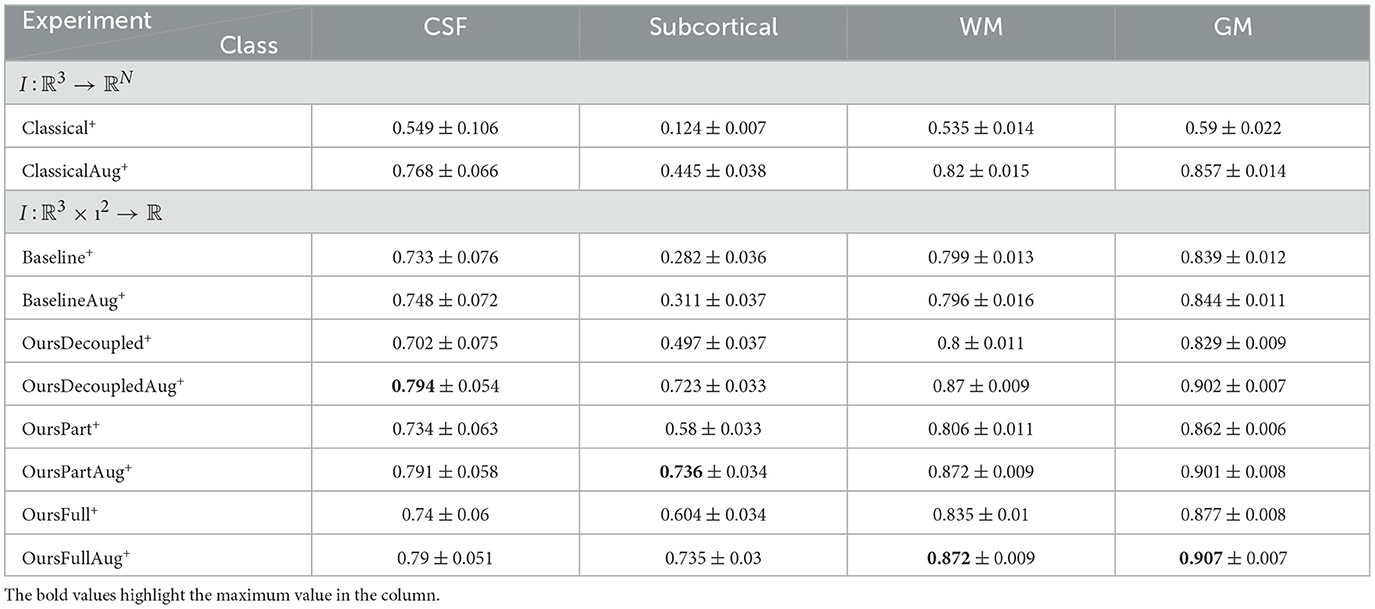
Table 9. Statistics of dice scores from experiments using rotated data and models of high capacity.

Table 10

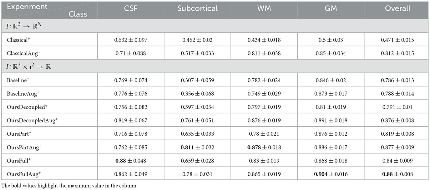
Table 10. Statistics of classification accuracy from experiments using rotated data and models of high capacity.

It is worth noticing that Baseline models almost do not suffer from performance drop while applied with rotated data. It is an SO(3)-network that preserves rotational equivariance on S². For a single-voxel input, the network is very resistant to variations, but the performance of this model is limited due to the lack of spatial interaction and thus in general worse than models with spatial interplay.

Examples of predictions using the rotated test set can be found in Figure 6B. It is easily observed that the classical CNN does not generalize well to the data variation, while models with rotational symmetry (either SO(3), 𝕋³ × SO(3), or SE(3)) generate better results. However, it is also noticeable that for a challenging minority class, subcortical region, OursFull⁺ performs better than the others while other models with some rotational equivariance do not predict a concentrated subcortical region. Zoom-in examples can be found in Figure 7. Predictions from Baseline are omitted from Figure 7 since it does not have the same level of performance.

Figure 7

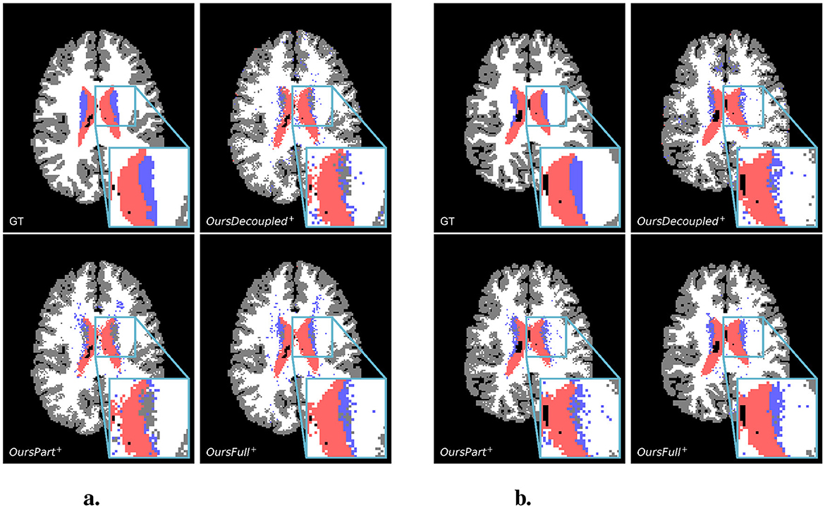
Figure 7. Showcases of zoom-in regions from predictions of the rotated test set. For both scan slices presented, from left to right, top to bottom, are the ground truth, prediction from OursDecoupled⁺, OursPart⁺, and OursFull⁺. The colors of different regions are the same as in Figure 6. (A) A test scan slice. (B) Another test scan slice.

4.3.7.1 Augmentation in training data vs. augmentation in testing data

We have experimented models trained with both the original training set and augmented training set, and models tested with both the original test set and randomly rotated test set. The random rotations applied to the test set can be seen as augmentation too. As was discussed above, data augmentation changes the distribution of the dataset, which creates inconsistency between the training and testing set. However, augmentation in the training set enables the models to see more data and thus even tested with the original test set, the performance of any model does not go far off, since the model has seen the type of data in the test set. The performance of models trained with data augmentation is worse than that of models trained with the original training set, though, due to the inconsistency of distributions between the training set and test set when only one of them is augmented. Figure 8A shows, for models tested with the original test set only, the decrease of model performance from models trained with the original training set to models trained with data augmentation. The y-axis shows the logistic map of the ratio of the performance decrease and is calculated by $L(x)=\frac{1}{e^{-\alpha x}}$ with α = 20, $x=\frac{C_{original}}{C_{augmented}}$, and C_original and C_augmented are the numbers indicating the performance (in this case, either dice score or accuracy as shown in the figure) of models tested with only the original test set but trained with the original (C_original) or augmented (C_augmented) training set. We can see from Figure 8A that the performance of the equivariant models we propose decrease less. This shows, from one perspective, the resistance of equivariant models to inconsistency of data distributions between training and testing data. On the other hand, having data augmentation only in the test set becomes a big problem for models without equivariance. Figure 8B shows, for models trained with the original training set only, the performance decrease from models tested with the original test set to those tested with rotated data. The y-axis values are calculated the same as the formula above, but the C_original and C_augmented become the numbers indicating the performance of models trained with the original training set only but tested with the original (C_original) or rotated (C_augmented) test set. We can see clearly from Figure 8B as well that the performance of classical CNN decreases the most using rotated data, and the decrease of performance goes down when we enforce more spatial equivariance in the model. Baseline models decrease the least, but again, the performance is limited due to the lack of information in ℝ³. Furthermore, the SE(3)-equivariance is implemented separately for the spatial and spherical parts and is with interpolation in the spatial part; thus, there are some errors introduced to it. Therefore, OursFull models always perform the best when there is variation in the test data.

Figure 8

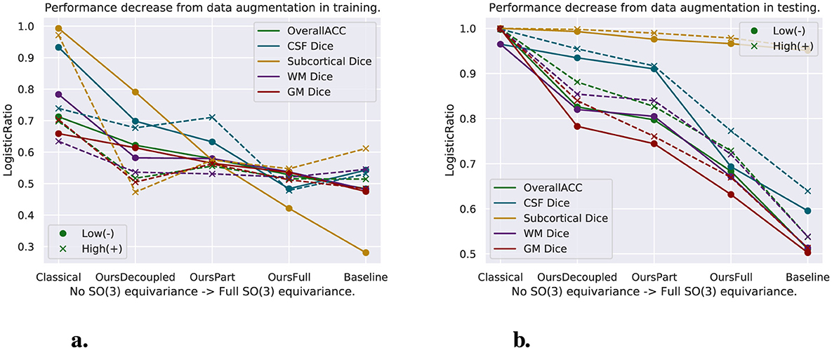
Figure 8. Logistic map of the ratio of two criteria to evaluate the proposed models. One criterion is for the models trained with augmented data compared to their counterparts trained with original data. For models trained both with original and augmented data, the left figure shows the decrease of test results while trained with data augmentation and tested with the original test set as shown in Tables 3–6. The second criterion is for the models trained with original data only. It is the decrease of performance while tested with rotated data, shown on the right figure. (A) Model performance decrease while trained with data augmentation. (B) Model performance decrease while applied with rotated test set.

4.3.7.2 Rotational invariance for Type 1 discretization

Furthermore, we have also experimented with networks that have some rotational invariance but in the classical CNN setup - viewing the DWI images as I:ℝ³ → ℝ^N. Taking the classical CNN setup we have in Section 4.2.1, we rotate the CNN kernels in each layer using the same rotations as in Section 4.2.4 to discretize SO(3). As was done above, we use the 60 rotations from the icosahedral symmetry group as well as only 12 of them (1 at each rotation axis) to act on the CNN kernels. In each layer, one rotation of the kernel is only convolved with the response of the corresponding rotation from the last layer; thus, this network is in fact 60 (or 12) independent networks, in which they share the same weights of different rotations. At the end, we take the average of the 60 (or 12) responses from all the rotations. With a small trial, we discovered that, as expected, even though this type of network does not perform as well as our spatial-directional GCNN as a whole, the performance decreases little in the full icosahedral group case with 60 rotations when tested with augmented data and decreases more when only a subset (12) of the group is used to rotate the kernels (see Table 11).

Table 11

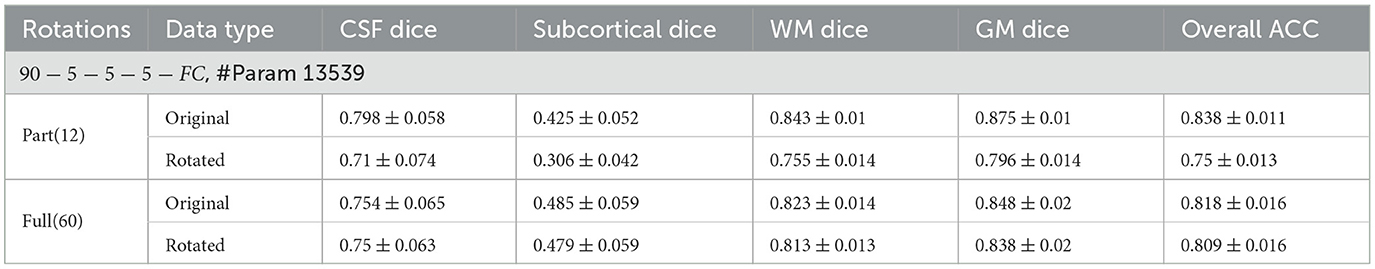
Table 11. Augmented CNN tested with original and rotated data.

This further demonstrates that having rotational equivariance in the model makes it much more robust to variance in the data - which, with no need of explanation, is inevitable when dealing with real-world raw data. Averaging rotational copies of a classical CNN achieves the goal of dealing with variance in data, but for non-linear data such as DWI, for which signals in voxels have some geometric structure, our full SE(3)-GCNN provides the best solution.

4.4 Comparison to state-of-the-art

We now compare our method to the approach of Müller et al. (2021). They used DWI data with q-space encoding in the diffusion part and the spatial part of the data is referred to as p-space, and these two parts of the data resemble the S² and ℝ³ spaces in our formulation. We use the b-vectors from the HCP dataset as the input to the q-space. In their case, the input of the network is a whole DWI scan, not a series of extracted patches like we do, and we cannot fit an entire HCP scan into the model without exceeding the memory limit of a 24 GB GPU. After discussion and agreement with one of the authors (V. Golkov), we decided to use a modified architecture of their network to get an as fair as possible comparison: (1) we provide their network with patches of the same size as ours (7 × 7 × 7), but with DWI signals that are only normalized by b0 instead of interpolated spherical functions in each voxel like we did in our method. (2) The best performing model hyper-parameters they provided in the paper (with 4 and 5 layers in totals) are optimized for receptive fields that are much larger than ours, we use instead their 3-layer network, which has almost the same level of performance. (3) We have also disabled padding in their network to cancel biases introduced in the networks. After 3 p-spatial layers, the output of their network without padding has spatial dimensions 1 × 1 × 1. Their method and ours thus perform the same task: voxel-wise classification. We used the Focal Loss (Lin et al., 2018) using the same parameters as all the experiments above. We used the suggested structure of their network with fully connected layers in the radial basis, which reportedly has better performance than ones without them. To make the comparison fair, we use a network whose hyper-parameters are different from what was presented in Liu et al. (2022) such that the number of trainable parameters is similar to that of Müller et al. (2021).

4.4.1 Network architectures

For Müller et al. (2021), we use the 1(pq)+1(q−reduction)+2(p) layer structure with the TP±1 basis presented in their paper and channels (5, 3, 0, 0), (5, 3, 0, 0), (10, 5, 0, 0), (4, 0, 0, 0) as presented in the Appendix section E.1 in their paper, except that we changed the output channel to 4 to fit our multiclass classification task and changed the p-space kernel sizes to 3 to ensure that the receptive field of the network is 7 × 7 × 7, as we discussed with the author. For our method, we use a ReLU(lift)−ReLU(gconv)−ReLU(gconv)−project−FC architecture such that there are three spatial layers as in Müller et al. (2021). With each layer split into 2, we use 10 − 10 − 20 − 40 − 20 − 10−proj.−4 as our layer structure such that we have similar numbers of parameters as Müller et al. (2021). Our method has 34964 parameters, while Müller et al. (2021) has 34,781 parameters.

4.4.2 Results

The results are shown in Table 12. We can see that our method performs better than Müller et al. (2021). To test the equivariance of both methods, we again test both models with the randomly rotated test set as presented above, and the results can be found in Table 13.

Table 12

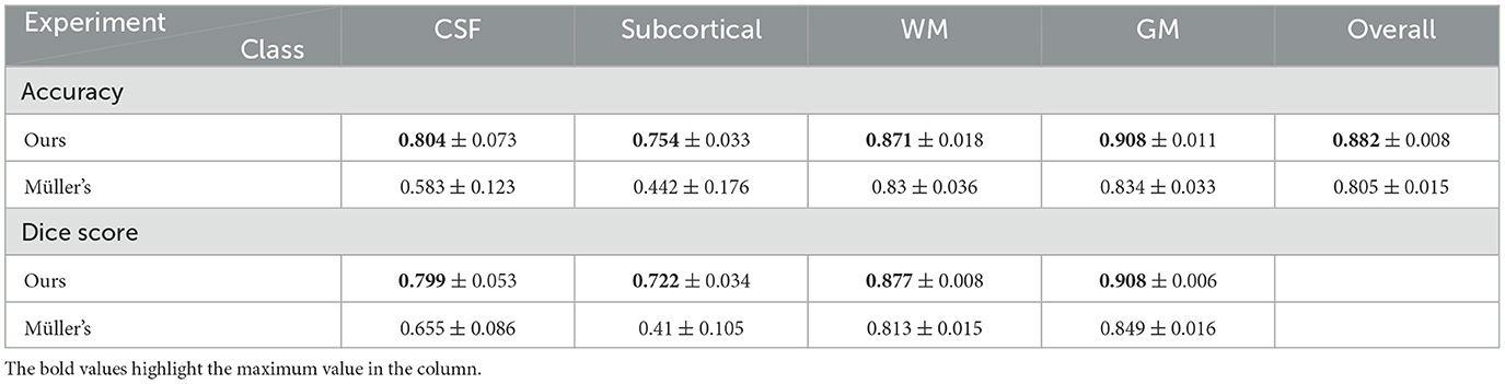
Table 12. Statistics of results from both our method and Müller's method.

Table 13

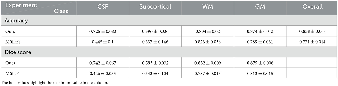
Table 13. Statistics of results from both our method and Müller's method tested with rotated test set.

We can see from the numbers that the performance of Müller et al. (2021) does not drop much either while tested with unseen rotated test set, similar to our method. As we can see from Figure 9, overall, Müller et al. (2021) lost less in percentage of the Dice scores of Subcortical, White matter, and overall accuracy but more in CSF Dice score. Both equivariant methods are more resistant to variations in the distributions of the training and test set than the non-equivariant models presented above. Moreover, since the overall performance decrease of Müller et al. (2021) while tested with rotated data is lower than our fully equivariant model, Müller et al. (2021) actually has better equivariance than all models we presented even though their prediction accuracies and dice scores are lower.

Figure 9

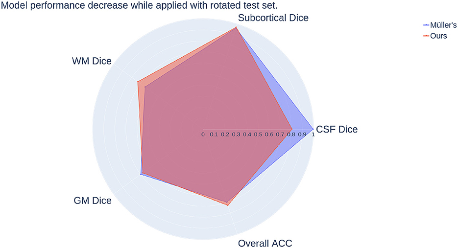
Figure 9. Comparison of model performance decrease while applied with rotated test set between our method and Müller's. The radial axis indicates the decrease, and it is the logistic map of the ratio calculated by the same scheme used in Figure 8.

4.5 Comparison to non-NN spherical harmonics feature classification

Following the method described in their paper, we extracted spherical harmonic features from each voxel of b−1000 DWIs and used SVMs for classification. Both one-vs-one and one-vs-all SVM configurations were applied to evaluate their comparative effectiveness in handling multiclass data. To normalize features, we experimented with both standard and min-max normalization methods. The performance of each setup was assessed using accuracy and Dice score metrics, consistent with the evaluation metrics for our proposed method. The results are shown in Table 14.

Table 14

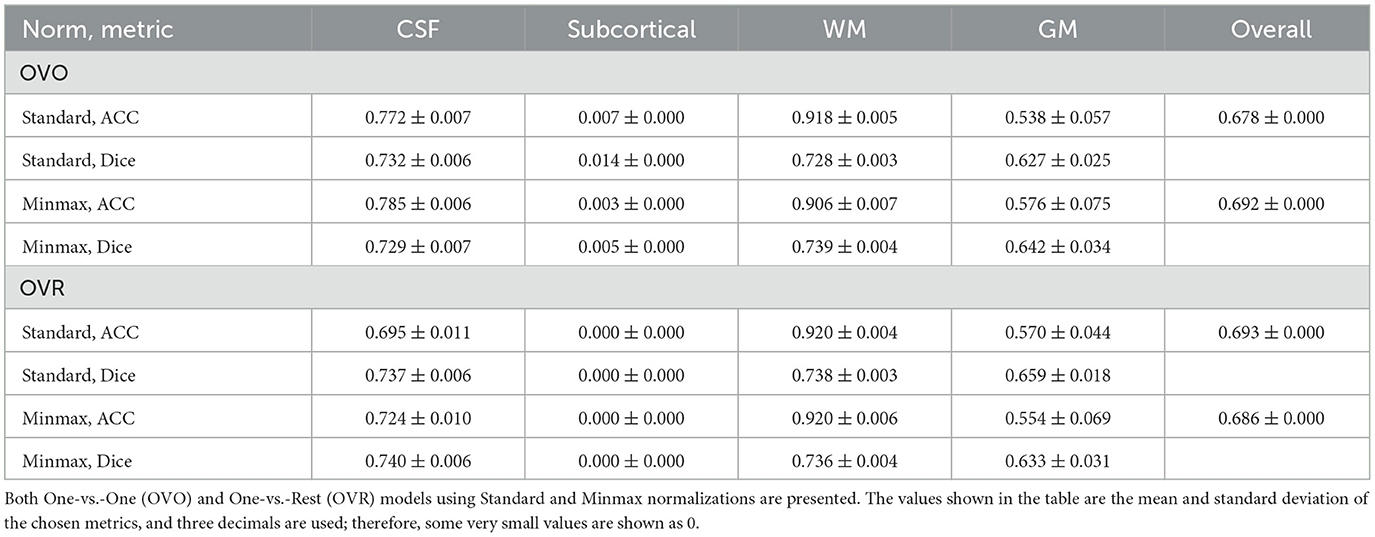
Table 14. Results for all models from Schnell et al. (2009) for b = 1000.

As shown in Table 14, the performance of the method from Schnell et al. (2009) is significantly lower than that of our proposed approach. In particular, for the challenging class–the subcortical region–the model showed minimal recognition capability. This result is expected as the rotation-invariant features derived independently from individual voxels inherently disregard the spatial relationships among voxels, which undermines model robustness. Furthermore, our SO(3) models, which similarly do not incorporate spatial voxel connectivity, nonetheless outperform the method in Schnell et al. (2009), underscoring the robustness and stability introduced by the equivariant convolutions within our model.

5 Discussion

The resistance to data variation that has been shown by our fully equivariant network was demonstrated on synthetically augmented data - with 90-degree rotations. Even though this synthetic augmentation did not cost any loss of signals or any interpolation-caused inaccuracy, it is desirable to verify the robustness of more complex group actions in CNNs using data with real-world variations (e.g., subjects scanned in different positions, affine variations in shapes). Acquiring this type of data is another challenge. On the other hand, data augmentation seems to be very robust against the variations in the rotated test set. However, this is because the augmentations applied in the training set and the test set are identical, and they modeled exactly the same distribution in the data. Our proposed equivariant methods deal with inconsistent distributions between the training set and the test set much better, which is usually the case in real world. In addition, our method outperforms (Müller et al., 2021) with the same amount of information given to the models. Even though both methods show similar resistance to variations in the distributions of the training and test set, our model has a more light-weight implementation using regular group representation with separable kernels. Furthermore, the experiments we conducted using Schnell et al. (2009) have shown the power of equivariant learning in non-Euclidean spaces. Using rotation-invariant features as in Schnell et al. (2009) is beneficial in terms of getting consistent features from spherical functions, regardless of the orientation. However, extracting invariant features from the very beginning also discards potentially valuable orientational information that is implicitly embedded in the data, and discarding spatial information completely severely weakens the capability of the model. This is easily shown by the fact that our SO(3) models that also discard spatial relationships outperform (Schnell et al., 2009).

In conclusion, we presented a systematic study of GCNNs of various group actions with the application to DWI segmentation. We interpreted images of DWI scans (I:ℝ³×S² → ℝ) as functions in the homogeneous spaces of groups with different complexities of symmetries and provided a detailed analysis of how different levels of complexities of these symmetries impact the performance of the network. It is shown from the models OursDecoupled and OursFull that whether or not more complex transformations should be imposed in the model is not always a clear-cut, since while tested on the original test set, OursDecoupled has a slightly better performance. OursDecoupled incorporates a mathematically well-defined, but physically impossible group action, yet it is computed more cheaply, while OursFull incorporates the SE(3) action, which corresponds to the expected physical transformations of the data. And, under any physically realistic turbulence in the test data resulting in unseen distributions, adding to the model possible transformations of the data (to the limit of their discretizations) provides a more stable performance. Therefore, we emphasize the importance of imposing the full roto-translation transformations in models as it is the kind that appears in the data. From the experiments, we conclude that (1) exploiting the spatial-directional interactions in the data is crucial for efficient learning of the features; (2) incorporating complex group actions of 3D rigid motions—SE(3)—might not be essential for highly aligned and preprocessed data such as the human connectome project (HCP) (Van Essen et al., 2013), but it shows significantly higher resistance to variations in data. For real-world raw data in which the positions of subjects are not perfectly aligned as in Van Essen et al. (2013), our proposal shows significant potential.

Data availability statement

The original contributions presented in the study are included in the article/Supplementary material, further inquiries can be directed to the corresponding author.

Ethics statement

The studies involving humans were approved by Connectome Coordination Facility. The studies were conducted in accordance with the local legislation and institutional requirements. Written informed consent for participation was not required from the participants or the participants' legal guardians/next of kin in accordance with the national legislation and institutional requirements.

Author contributions

RL: Conceptualization, Formal analysis, Investigation, Methodology, Project administration, Resources, Software, Validation, Visualization, Writing – original draft, Writing – review & editing. FL: Formal analysis, Methodology, Supervision, Writing – original draft, Writing – review & editing. EB: Conceptualization, Methodology, Visualization, Writing – review & editing. SD: Funding acquisition, Project administration, Resources, Supervision, Writing – review & editing. KE: Funding acquisition, Resources, Supervision, Writing – review & editing.

Funding

The author(s) declare financial support was received for the research, authorship, and/or publication of this article. This project has received funding from the European Union's Horizon 2020 research and innovation program under the Marie Sklodowska-Curie grant agreement No. 801199. This study only contains the author's views. The Research Executive Agency and the Commission are not responsible for any use that may be made of the information it contains. Data were provided [in part] by the Human Connectome Project, WU-Minn Consortium (Principal Investigators: David Van Essen and Kamil Ugurbil; 1U54MH091657) funded by the 16 NIH Institutes and Centers that support the NIH Blueprint for Neuroscience Research; and by the McDonnell Center for Systems Neuroscience at Washington University. This project is also partially funded by 3Shape A/S, as well as by the research program VENI (grant number 17290), financed by the Dutch Research Council (NWO).

Acknowledgments

We would like to thank Dr. Vladimir Golkov for his efforts and insights in helping us setting up experiments with their model (Müller et al., 2021).

Conflict of interest

The authors declare that the research was conducted in the absence of any commercial or financial relationships that could be construed as a potential conflict of interest.

Publisher's note

All claims expressed in this article are solely those of the authors and do not necessarily represent those of their affiliated organizations, or those of the publisher, the editors and the reviewers. Any product that may be evaluated in this article, or claim that may be made by its manufacturer, is not guaranteed or endorsed by the publisher.

Supplementary material

The Supplementary Material for this article can be found online at: https://www.frontiersin.org/articles/10.3389/frai.2025.1369717/full#supplementary-material

References

Andrearczyk, V., Fageot, J., and Depeursinge, A. (2020). Local rotation invariance in 3D CNNs. Med. Image Analy. 65:101756. doi: 10.1016/j.media.2020.101756

PubMed Abstract | Crossref Full Text | Google Scholar

Aronsson, J. (2022). Homogeneous vector bundles and 𝒢-equivariant convolutional neural networks. Sampl. Theory Signal Process. Data Anal. 20.

Google Scholar

Banerjee, M., Chakraborty, R., Archer, D., Vaillancourt, D., and Vemuri, B. C. (2019). “DMR-CNN: a CNN tailored for DMR scans with applications to PD calssifiaction,” in 2019 IEEE 16th International Symposium on Biomedical Imaging (ISBI 2019) (Venice), 388–391. doi: 10.1109/ISBI.2019.8759558

Crossref Full Text | Google Scholar

Basser, P., Mattiello, J., and LeBihan, D. (1994). MR diffusion tensor spectroscopy and imaging. Biophys. J. 66, 259–267. doi: 10.1016/S0006-3495(94)80775-1

PubMed Abstract | Crossref Full Text | Google Scholar

Bekkers, E., Veta, M. L. M., Eppenhof, K., Pluim, J., and Duits, R. (2018). Roto-translation covariant convolutional networks for medical image analysis. Proc. MICCAI 2018, 440–448. doi: 10.1007/978-3-030-00928-1_50

PubMed Abstract | Crossref Full Text | Google Scholar

Bekkers, E. J. (2019). “B-spline CNNS on lie groups,” in International Conference on Learning Representations.

Google Scholar

Boscaini, D., Masci, J., Rodolà, E., and Bronstein, M. (2016). “Learning shape correspondence with anisotropic convolutional neural networks,” in 30th Annual Conference on Neural Information Processing Systems, NIPS 2016, eds. D. Lee, M. Sugiyama, U. Luxburg, I. Guyon and R. Garnett (Barcelona), 29.

PubMed Abstract | Google Scholar

Bouza, J. J., Yang, C.-H., Vaillancourt, D., and Vemuri, B. C. (2021). “A higher order manifold-valued convolutional neural network with applications to diffusion MRI processing,” in Information Processing in Medical Imaging, A. Feragen, S. Sommer, J. Schnabel, and M. Nielsen (Cham: Springer International Publishing), 304–317.

Google Scholar

Caruyer, E., and Verma, R. (2015). On Facilitating the Use of HARDI in Population Studies by Creating Rotation-Invariant Markers. Med. Image Anal. 20, 87–96. doi: 10.1016/j.media.2014.10.009

PubMed Abstract | Crossref Full Text | Google Scholar

Chakraborty, R., Banerjee, M., and Vemuri, B. (2018a). A CNN for homogeneous riemannian manifolds with application to neuroimaging. arXiv [Preprint]. arXiv:1805.05487.

Google Scholar

Chakraborty, R., Banerjee, M., and Vemuri, B. C. (2018b). H-CNNS: Convolutional neural networks for riemannian homogeneous spaces. arXiv [Preprint]. arXiv:1805.05487.05481. doi: 10.48550/arXiv.1805.05487

Crossref Full Text | Google Scholar

Chakraborty, R., Bouza, J., Manton, J., and Vemuri, B. C. (2020). Manifoldnet: A deep neural network for manifold-valued data with applications. IEEE Trans. Pattern Analy. Mach. Intellig. 44, 799–810. doi: 10.1109/TPAMI.2020.3003846

PubMed Abstract | Crossref Full Text | Google Scholar

Chen, H., Liu, S., Chen, W., Li, H., and Hill, R. (2021). Equivariant Point Network for 3D Point Cloud Analysis, 14514–14523.

PubMed Abstract | Google Scholar

Cohen, T., Geiger, M., Köhler, J., and Welling, M. (2018). “Spherical CNNs,” in International Conference on Learning Representations (Vancouver, BC).

Google Scholar

Cohen, T., Geiger, M., and Weller, M. (2020). “A general theory of equivariant CNNs on homogeneous spaces,” in Advances in Neural Information Processing Systems (NeurIPS 2019), 9142–9153.

Google Scholar

Cohen, T., and Welling, M. (2016a). Group equivariant convolutional neural networks. Int. Conf. Mach. Learn. 2016, 2990–2999. doi: 10.48550/arXiv.1602.07576

Crossref Full Text | Google Scholar

Cohen, T. S., Weiler, M, Kicanaoglu, B., and Welling, M. (2019). “Gauge equivariant convolutional networks and the icosahedral CNN,” in International Conference on Machine Learning (Long Beach, CA), 1321–1330.

Google Scholar

Cohen, T. S., and Welling, M. (2016b). Steerable CNNs. arXiv. doi: 10.48550/arXiv.1612.08498

Crossref Full Text | Google Scholar

Diestel, J., and Spalsbury, A. (2014). The Joys of Haar Measure. Amer Mathematical Society.

Google Scholar

Elaldi, A., Dey, N., Kim, H., and Gerig, G. (2021). “Equivariant spherical deconvolution: Learning sparse orientation distribution functions from spherical data,” in Information Processing in Medical Imaging, eds. A. Feragen, S. Sommer, J. Schnabel, and M. Nielsen (Cham: Springer International Publishing), 267–278.

PubMed Abstract | Google Scholar

Gens, R., and Domingos, P. (2014). Deep Symmetry networks. Vancouver: NIPS, 2537–2545.

Google Scholar

Gerken, J. E., Aronsson, J., Carlsson, O., Linander, H., Ohlsson, F., Petersson, C., et al. (2023). Geometric deep learning and equivariant neural networks. Artif. Intell. Rev. 56, 14605–14662. doi: 10.1007/s10462-023-10502-7

Crossref Full Text | Google Scholar

Golkov, V., Dosovitskit, A., Sperl, J. I., Menzel, M. I., Czisch, M., Särmann, P., et al. (2016). q-space deep learning: twelve-fold shorter and model-free diffusion MRI scans. IEEE Trans. Med. 35, 1344–1351. doi: 10.1109/TMI.2016.2551324

PubMed Abstract | Crossref Full Text | Google Scholar

Graham, S., Epstein, D., and Rajpoot, N. (2020). Dense steerable filter cnns for exploiting rotational symmetry in histology images. IEEE Trans. Med. Imaging 39, 4124–4136. doi: 10.1109/TMI.2020.3013246

PubMed Abstract | Crossref Full Text | Google Scholar

Jupp, P. E., and Mardia, K. V. (1989). A unified view of the theory of directional statistics, 1975-1988. Int. Statist. Rev. 57, 261–294. doi: 10.2307/1403799

Crossref Full Text | Google Scholar

Knigge, D. M., Romero, D. W., and Bekkers, E. J. (2022). “Exploiting redundancy: separable group convolutional networks on lie groups,” in Proceedings of the 39th International Conference on Machine Learning, eds. K. Chaudhuri, S. Jegelka, L. Song, C. Szepesvari, G. Niu, and S. Sabato (New York: PMLR), 11359-11386.

Google Scholar

Kondor, R., and Trivedi, S. (2018). “On the generalization of equivariance and convolution in neural networks to the action of compact groups,” in International Conference on Machine Learning (Stockholm), 2747–2755.

Google Scholar

Lin, T.-Y., Goyal, P., Girshick, R., He, K., and Dollár, P. (2018). Focal loss for dense object detection. IEEE Trans. Pattern Anal. Mach. Intell. 42, 318–327. doi: 10.1109/TPAMI.2018.2858826

PubMed Abstract | Crossref Full Text | Google Scholar

Liu, R., Lauze, F., Erleben, K., and Darkner, S. (2021). “Bundle geodesic convolutional neural network for dwi segmentation from single scan learning,” in Computational Diffusion MRI, eds. S. Cetin-Karayumak, D. Christiaens, M. Figini, P. Guevara, N. Gyori, V. Nath, and T. Pieciak (Cham: Springer International Publishing), 121–132.

Google Scholar

Liu, R., Lauze, F. B., Bekkers, E. J., Erleben, K., and Darkner, S. (2022). “Group convolutional neural networks for DWI segmentation,” in Geometric Deep Learning in Medical Image Analysis (Strasbourg).

Google Scholar

Masci, J., Boscaini, D., Bronstein, M., and Vandergheynst, P. (2015). “Geodesic convolutional neural networks on riemannian manifolds,” in 2015 IEEE International Conference on Computer Vision Workshop (ICCVW) (Santiago), 832–840. doi: 10.1109/ICCVW.2015.112

Crossref Full Text | Google Scholar

Müller, P., Golkov, V., Tomassini, V., and Cremers, D. (2021). Rotation-Equivariant Deep Learning for Diffusion MRI. ISMRM.

Google Scholar

Novikov, D., Veraart, J., Jelescu, I., and Fieremans, E. (2018). Rotationally-invariant mapping of scalar and orientational metrics of neuronal microstructure with diffusion MRI. Neuroimage 174, 518–538. doi: 10.1016/j.neuroimage.2018.03.006

PubMed Abstract | Crossref Full Text | Google Scholar

Poulenard, A., Ovsjanikov, M., and Guibas, L. J. (2022). Equivalence between Se(3) equivariant networks via steerable kernels and group convolution. arXiv [Preprint] arXiv:2211.15903.

Google Scholar

Schnell, S., Saur, D., Kreher, B. W., Hennig, J., Burkhardt, H., and Kiselev, V. G. (2009). Fully automated classification of hardi in vivo data using a support vector machine. Neuroimage 46:642–651. doi: 10.1016/j.neuroimage.2009.03.003

PubMed Abstract | Crossref Full Text | Google Scholar

Schonsheck, S. C., Dong, B., and Lai, R. (2018). Parallel transport convolution: a new tool for convolutional neural networks on manifolds. arXiv [Preprint] arXiv:1805.07857.

Google Scholar

Schwab, E., Cetingül, H. E., Asfari, B., and Vidal, E. (2013). “Rotational invariant features for HARDI,” in Information Processing in Medical Imaging. Lecture Notes in Computer Science, Vol. 7917 (Berlin; Heidelberg: Springer).

Google Scholar

Sedlar, S., Alimi, A., Papadopoulo, T., Deriche, R., and Deslauriers-Gauthier, S. (2021). “A spherical convolutional neural network for white matter structure imaging via dMRI,” in Medical Image Computing and Computer Assisted Intervention-MICCAI 2021, eds. M. de Bruijne, P. C. Cattin, S. Cotin, N. Padoy, S. Speidel, Y., Zheng, and C. Essert (Cham: Springer), 529–539.

Google Scholar

Sedlar, S., Papadopoulo, T., Deriche, R., and Deslauriers-Gauthier, S. (2020). “Diffusion MRI fiber orientation distribution function estimation using voxel-wise spherical U-net,” in International MICCAI Workshop 2020 - Computational Diffusion MRI (Lima: MICCAI).

Google Scholar

Skibbe, H., and Reisert, M. (2017). Spherical tensor algebra: a toolkit for 3d image processing. J. Math. Imaging Vis. 58, 349–381. doi: 10.1007/s10851-017-0715-7

Crossref Full Text | Google Scholar

Smets, B. M. N., Portegies, J., Bekkers, E. J., and Duits, R. (2021). PDE-based Group Equivariant Convolutional Neural Networks. Cham: Springer.

Google Scholar

Sommer, S., and Bronstein, A. (2020). Horizontal flows and manifold stochastics in geometric deep learning. IEEE Trans. PAMI. 44, 811–822. doi: 10.1109/TPAMI.2020.2994507

PubMed Abstract | Crossref Full Text | Google Scholar

Tuchs, D. S. (2004). Q-ball imaging. Magnet. Reson. Med. 52, 1358–1372. doi: 10.1002/mrm.20279

PubMed Abstract | Crossref Full Text | Google Scholar

Van Essen, D. C., Smith, S. M., Barch, D. M., Behrens, T. E., Yacoub, E., and Ugurbil, K. (2013). The WU-Minn human connectome project: an overview. Neuroimage 80, 62–79. doi: 10.1016/j.neuroimage.2013.05.041

PubMed Abstract | Crossref Full Text | Google Scholar

Weiler, M., Forré, P., Verlinde, E., and Welling, M. (2021). Convolutional networks-isometry and gauge equivariant convolutions on riemannian manifolds. arXiv [Preprint] arXiv:2106.06020. doi: 10.48550/arXiv.2106.06020

Crossref Full Text | Google Scholar

Weiler, M., Geiger, M., Welling, M., Boomsma, W., and Cohen, T. (2018a). “3D steerable CNNs: learning rotationally equivariant features in volumetric data,” in Advances in Neural Information Processing Systems, 10401–10412.

Google Scholar

Weiler, M., Hamprecht, F., and Storath, M. (2018b). “Learning steerable filters for rotation equivariant CNNS,” in 2018 IEEE/CVF Conference on Computer Vision and Pattern Recognition (Salt Lake City, UT: IEEE), 849–858.

Google Scholar

Worrall, D., Garbin, S., Turmukhambetov, D., and Brostow, G. (2017). “Harmonic networks: deep translation and rotation equivariance,” in 2017 IEEE Conference on Computer Vision and Pattern Recognition (CVPR) (Honolulu, HI: IEEE).

Google Scholar

Zucchelli, M., Deslauriers-Gauthier, S., and Deriche, R. (2020). A computational framework for generating rotation invariant features and its application in diffusion MRI. Med. Image Anal. 60:101597. doi: 10.1016/j.media.2019.101597

PubMed Abstract | Crossref Full Text | Google Scholar