Impact of Box-Cox Transformation on Machine-Learning Algorithms

This paper studied the effects of applying the Box-Cox transformation for classification tasks. Different optimization strategies were evaluated, and the results were promising on four synthetic datasets and two real-world datasets. A consistent improvement in accuracy was demonstrated using a grid exploration with cross-validation. In conclusion, applying the Box-Cox transformation could drastically improve the performance by up to a 12% accuracy increase. Moreover, the Box-Cox parameter choice was dependent on the data and the used classifier.

Introduction

Feature transformation can improve the performance of a machine learning algorithm. Simple transformations already had a significant impact on classification performance (Bicego and Baldo, 2016; Liang et al., 2020). Motivated by their findings, the impact of the Box-Cox transformation for classification tasks was studied. Often, Box-Cox is used to increase the Gaussianity of data. This can help in some special cases; however, we observed that transformations that do not maximize the Gaussianity of the data are often superior for classification accuracy. Additionally, Bicego and Baldo (2016) have shown that the Gaussianity of datasets is not critical and by allowing the effect of the Box–Cox transformation work in operational ranges that do not necessarily correspond to an increase in Gaussianity, they have shown that class separability can be improved. Furthermore, they proposed an automatic procedure for obtaining an optimal transformation. Their procedure relied on the spherical and diagonal optimization of statistical measurements, such as maximum likelihood or Fisher criterion. They showed that both are capable of improving the classification result, although the diagonal case often gives higher accuracy. This can be expected due to the higher number of parameters. Furthermore, they demonstrated that the choice of optimization criteria depends on the classifier itself.

Gao et al. (2017) attempted to find the optimal Box-Cox transformation in big data. They focused on regression and tried to get a maximum likelihood estimation (MLE) for the Box-Cox parameter when the dataset is massive. By using MapReduce, they proposed an algorithm that can be run in parallel and is able to process big data in chunks.

Cheddad (2020) investigated the effect of the Box-Cox transformation on images. They proposed an image pre-processing tool by using the Box-Cox transformation for histogram transformation. The parameters for the transformation were calculated using the MLE. By using image histograms instead of the image data, the time complexity could be kept static, and thus independent of the size of the image.

However, our focus is on the classification of tabular data that fits into the main memory. We sought to explore a generalization of the approach from Bicego and Baldo (2016) and provide an optimization procedure that is classifier dependent.

Box-Cox Transformation

The original Box-Cox transformation is a one-dimensional transformation with one parameter often called λ and is applied element-wise to a vector y (Box and Cox, 1964):

$\begin{array}{l}\text{Let }y\in {ℝ}^n\text{ and }\lambda \in ℝ\\ y_i^{(\lambda )}=\{\begin{array}{ll}\frac{y_i^{(\lambda )}-1}{\lambda }\hfill & \text{if }\lambda \ne \text{0}\hfill \\ \ln \left(y_i\right)\hfill & \text{if }\lambda \text{=0}\hfill \end{array}\end{array}$

Many different criteria have been proposed for an optimal λ. The most used method, which was introduced by Box and Cox (1964), is a MLE. Other approaches include a Bayesian approach (Sweeting, 1984), robust estimators, Carroll and Ruppert (1985), Lawrance (1988), and Kim et al. (1996) and an attempt to iteratively maximize Gaussianity (Vélez et al., 2015). The Box-Cox transformation is mostly studied for regression tasks. For λ>1 the transformation is convex and for λ <1 the transformation is concave. As described by Bicego and Baldo (2016), the data is stretched in the positive direction for λ>1 and stretched in the negative direction for λ <1. Assuming the data is range standardized between 1 and 2, this means for λ>1 that data points near 1 have a smaller relative distance than points near 2 after applying the Box-Cox transformation (Bicego and Baldo, 2016). The opposite behavior holds for λ <1 (Bicego and Baldo, 2016). For λ = 1 the data is only shifted by 1 in the negative direction. The Box-Cox transformation is monotonic and therefore does not change the ordering of the data. These properties might help to increase class separability. For multi-dimensional data, X∈ℝ^n×p, it is usually applied p times as 1-dimensional mapping to each column with different values for λ. Therefore, the overall transformation is specified by a p-dimensional vector, Λ = [λ₁, λ₂, …, λ_p].

The optimization of the parameter vector Λ can be done in several ways. Naturally, one could optimize λ_i of the corresponding column X_i independently with traditional criteria such as MLE (Box and Cox, 1964) or the Bayesian approach (Sweeting, 1984). This will be referred to as diagonal setting,

$\begin{array}{ll}{\Lambda }^{*}=\left[\begin{array}{c}{\lambda }_1^{*}\\ {\lambda }_2^{*}\\ ...\\ {\lambda }_p^{*}\end{array}\right]=\left[\begin{array}{c}{\displaystyle \underset{{\lambda }_1}{argmin}}L({\lambda }_1,X_1)\\ {\displaystyle \underset{{\lambda }_2}{argmin}}L({\lambda }_2,X_2)\\ ...\\ {\displaystyle \underset{{\lambda }_p}{argmin}}L({\lambda }_p,X_p)\end{array}\right]& (1)\end{array}$

where L(·, ·) is a criterion that needs to be minimized. A simplification of this case is the spherical setting. Only a scalar value λ gets optimized and applied to every column.

$\begin{array}{ll}{\lambda }^{*}={\displaystyle \underset{\lambda }{argmin}}{\displaystyle \sum _{i=1}^{i=p}}L(\lambda ,X_i)& (2)\end{array}$

The most general case is called full and optimizes.

$\begin{array}{ll}{\Lambda }^{*}=\left[\begin{array}{c}{\lambda }_1^{*}\\ {\lambda }_2^{*}\\ ...\\ {\lambda }_p^{*}\end{array}\right]=\left[\begin{array}{c}{\displaystyle \underset{{\lambda }_1}{argmin}}L(\Lambda ,X)\\ {\displaystyle \underset{{\lambda }_2}{argmin}}L(\Lambda ,X)\\ ...\\ {\displaystyle \underset{{\lambda }_p}{argmin}}L(\Lambda ,X)\end{array}\right]& (3)\end{array}$

Motivation

To demonstrate the influence of the Box-Cox transformation, a stratified cross validation with 10 folds and 5 repetitions was executed on various artificial 2-dimensional binary classification tasks with varying Λs. For each direction, i∈{1, 2}, λ_i was distributed evenly in the interval [−5, 5] with a spacing of 1. Hence, 11 × 11 accuracy estimates were conducted. Accuracy measurements were carried out for the different classifiers described in Table 1, as implemented in the Python library scikit-learn (Pedregosa et al., 2011). Additionally, the corresponding acronyms are given. Unless otherwise stated, the default parameters were used, and if provided, random seeds/states were set to 42. Python version 3.6.0, scikit-learn version 0.24.2, NumPy version 1.19.5, and SciPy version 1.5.4 were used.

TABLE 1

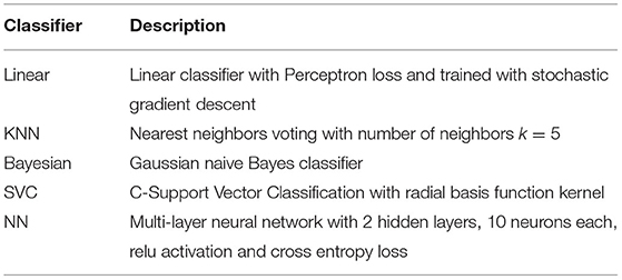
Table 1. Evaluated classifiers for a grid exploration and to test the proposed optimization method on real-world data: Details can be found in Pedregosa et al. (2011).

Figure 1 shows the different datasets that were used to study the accuracy for different values of Λ.

FIGURE 1

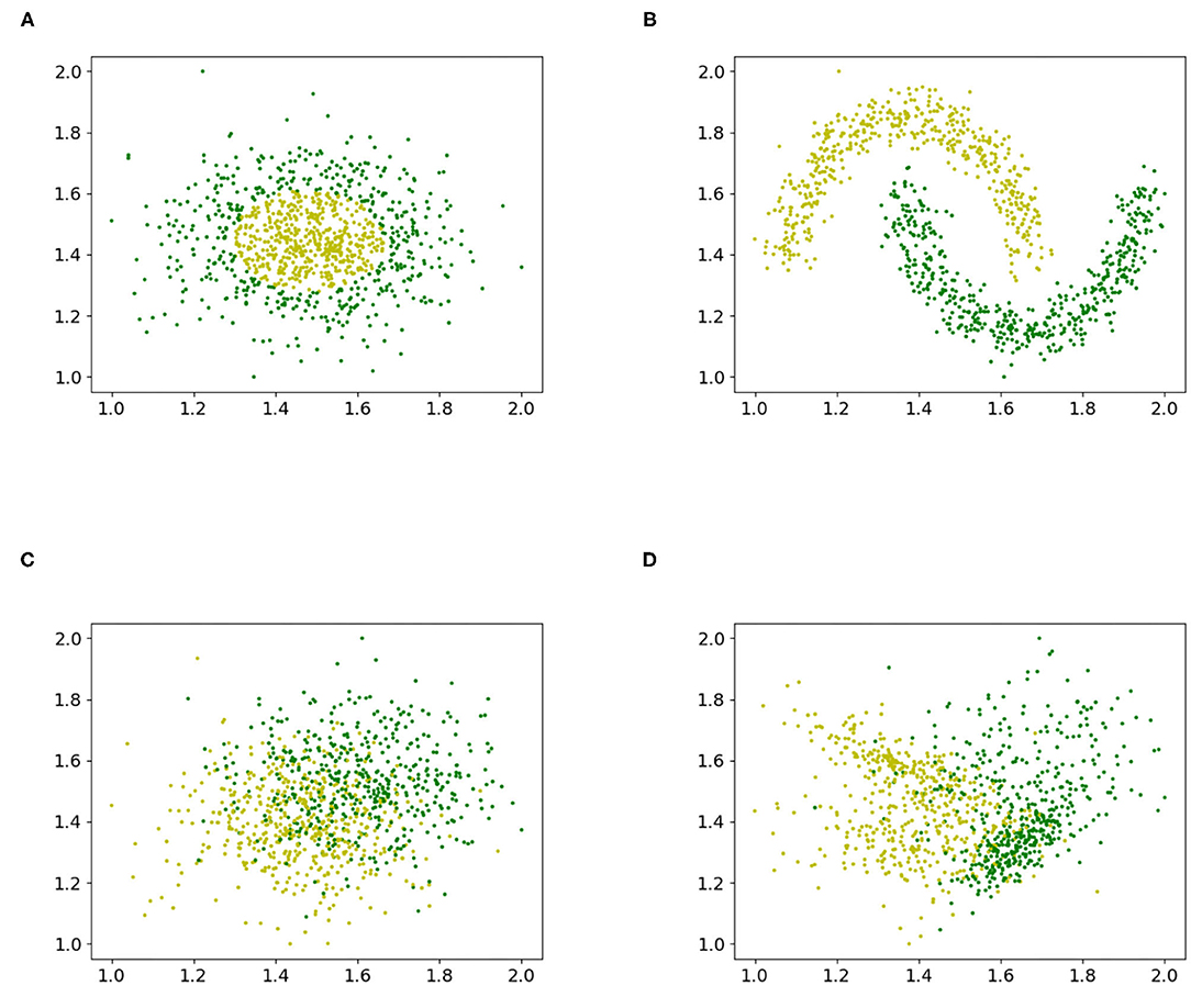
Figure 1. Various artificial binary classification problems were created to study the influence of the Box-Cox transformation with a grid exploration. (A) Gaussian quantiles, (B) interleaving half circles, (C) isotropic Gaussian blobs, and (D) random dataset.

Figure 2 shows the accuracy measurements for the exhaustive grid exploration of Λ on the random classification dataset Figure 1D. The corresponding pseudo-code is given in Algorithm 1. Before applying the Box-Cox transformation, all datasets were preprocessed with a range standardization between 1 and 2. This was done to show the exclusive behavior of the Box-Cox transformation without the influence of other effects; however, the transformation needed positive data. The upper range bound ensured that the features did not explode when transformed with a larger Λ. The results of the Box-Cox transformation were also standard scaled before being given to the classifiers.

FIGURE 2

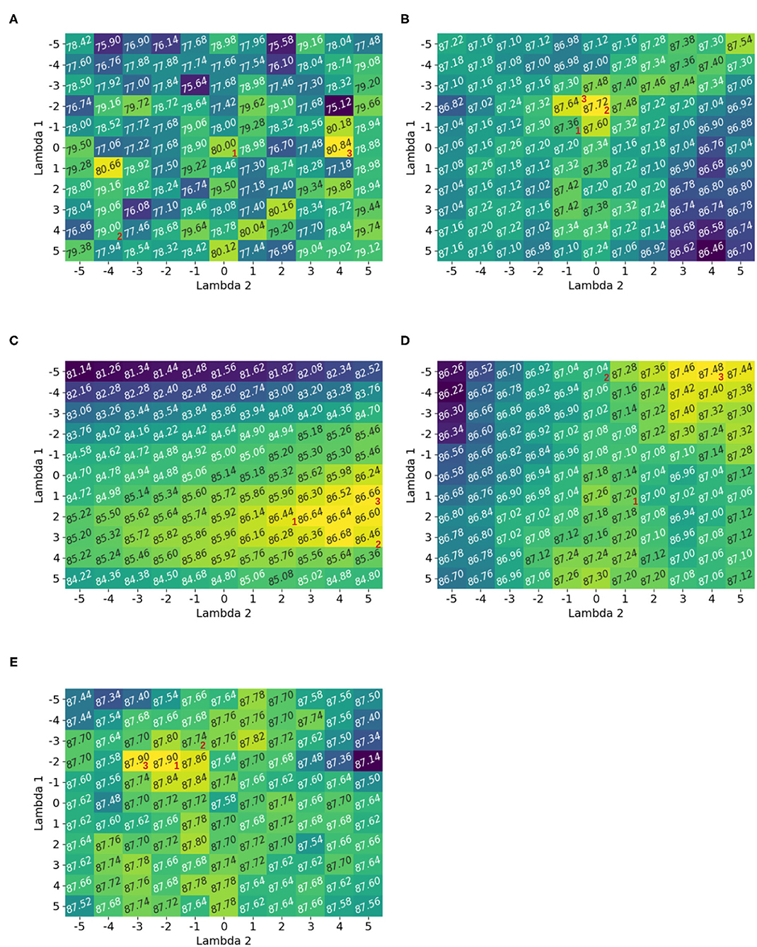
Figure 2. Accuracy heatmaps generated by Algorithm 1 for a random dataset. The numbers 1, 2, and 3 correspond to the optimal solution for the spherical, diagonal, and full optimization. If there are multiple solutions then only one possibility is shown. It was observed that the optimal parameter choice for the Box-Cox transformation depends on the classifier. The heatmaps showed multiple local maxima and full optimization led to the best optimization result. (A) Linear classifier, (B) KNN classifier, (C) Bayesian classifier, (D) SVC classifier, and (E) NN classifier.

ALGORITHM 1

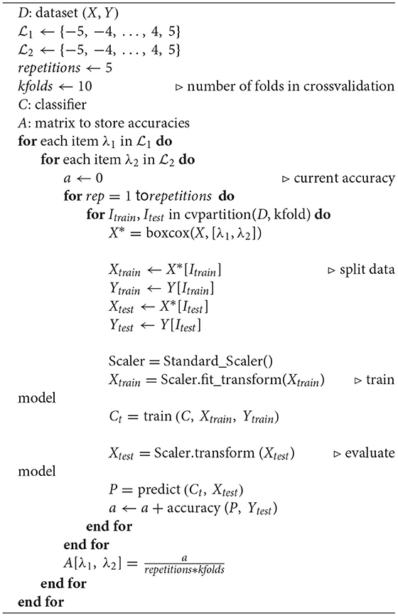
Algorithm 1 : 2D Accuracy Gridexploration

It was observed that the different heatmaps were not similar; hence, the Box-Cox transformation was dependent on the classifier itself. For example, Λ = [−5, 4] gave the best performance for the SVC classifier, but it was almost the worst for the neural network. While Λ = [1, 5] was the best for the Bayesian classifier, it was bad for the KNN classifier. This suggests that the optimization of the Box-Cox transformation was not only dependent on the data but also on the classifier. This observation was also made by Bicego and Baldo (2016).

The heatmaps also showed multiple local maxima. Hence, the optimization should be non-convex. Similar observations were made for the other datasets, and the corresponding heatmaps are provided in Appendix A.

Finally, it was obvious that the full optimization gave better results than the spherical and diagonal settings. The possible spherical configurations were seen on the diagonal of the heatmap (e.g., Λ∈{[−5, −5], [−4, −4], …, [5, 5]}). The diagonal can be illustrated by first fixing one direction λ_i = 1 and optimizing in the other direction and then vice versa. Possible optimal solutions for the spherical, diagonal, and full optimization were indicated with corresponding numbers 1, 2, and 3. If there were multiple options for the optimal solution in one direction for diagonal optimization, then the case that led to higher final optimization accuracy was used.

Table 2 summarizes the accuracy heatmaps for all four datasets in Figure 1. It shows the performance before applying the Box-Cox transformation and after applying the Box-Cox transformation with the best reported configuration of Λ. The numbers are rounded to the first decimal point. The accuracy before applying the Box-Cox transformation corresponds to a Box-Cox transformation with Λ = [1, 1] because this only shifts the data by 1 in each direction and therefore does not influence the classification result.

TABLE 2

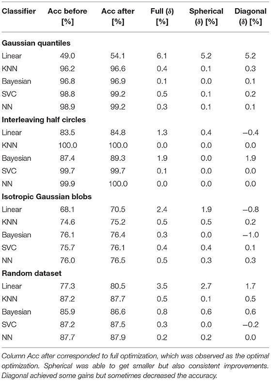
Table 2. Accuracy of five classifiers before and after applying Box-Cox transformation using three optimization strategies.

It was observed that the linear classifier benefited most from the Box-Cox transformation. The other classifiers also benefited, unless the classification result was almost perfect before applying the transformation (KNN and NN in the interleaving half circles dataset). Thus, Box-Cox transformation consistently improved the classification result.

It was also seen that, mostly, spherical optimization did not achieve the same improvements as full optimization. This is expected because of the lower number of parameters. In contrast, however, diagonal optimization resulted in even worse accuracies. This was observed, for example, for the linear classifier in the interleaving half circles dataset. Fixing in one direction and optimizing in the other direction resulted in an increase in accuracy (fixing λ₁ = 1 led to λ₂ = 4 with an improvement of 0.68%, and fixing λ₂ = 1 led to λ₁ = −3 with an improvement of 0.54%). However, combining the independent results led to Λ = [−3, 4] and a loss of accuracy of −0.36%. This can get arbitrarily bad because the outcome of a combination of the independent optimizations was unknown in advance.

To further study the behavior of the different optimization methods, the random dataset Figure 1D was generated 10 times with different random seeds and the accuracy for each optimization method was measured for the five classifiers given in Table 1 with a stratified cross validation with 10 folds and 5 repetitions. The average of the accuracy is given in Table 3.

TABLE 3

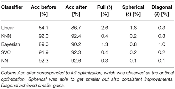
Table 3. Average accuracy of five classifiers before and after applying Box-Cox transformation using three optimization strategies for 10 times regenerated random dataset Figure 1D with different random seeds.

The Full optimization led consistently to the highest improvement in accuracy. Both Spherical and Diagonal optimization achieved an improvement for all classifiers. Diagonal optimization was better or equal than Spherical optimization for all classifiers except for the linear classifier.

Model and Optimization

The previous section showed that full optimization led to the best improvements. It was also demonstrated that the optimization was dependent on the classifier. Therefore, we propose a procedure for classifier-dependent multi-dimensional non-convex optimization. First, the general setup is described. Then, naive optimization is introduced. This was used as a baseline but suffered from the curse of dimensionality. Next, an iterative optimization is described that solved the dimensionality problem. Subsequently, various techniques for improving the iterative procedure are presented.

The general setup that was used with different optimization techniques consisted of a training function and a predicting function. It is shown in Algorithm 2. First, a model was trained to find the optimal parameter, Λ, for the Box-Cox transformation with a given classifier. Then the predicting function was used with the optimized Box-Cox parameter, Λ, to create predictions.

ALGORITHM 2

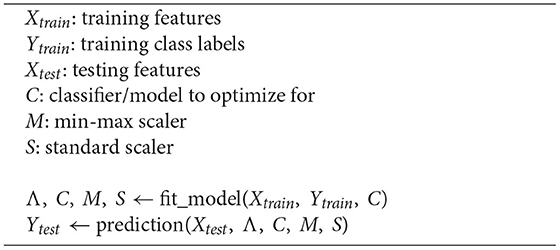
Algorithm 2 : Setup

The training procedure is given in Algorithm 3. It requires the features, the corresponding class labels, a classifier, and an optimization procedure for Λ. Suitable optimization procedures are given in Algorithm 5 (restricted to 2-dimensional data) and Algorithm 6 with further improvements for the latter in 6.1, 6.2, and 6.3. It first scaled the data into the range [1, 2] to ensure that the features were positive so that the Box-Cox transformation could be applied, and to ensure that the features did not explode at a larger Λ. Then, an optimization procedure was applied to find suitable values for Λ. As described in the previous section, this was dependent on the classifier itself. Next, the Box-Cox transformation was applied to the features with the optimized Λ. Then, the data were standard scaled to help classifiers that depended on a distance measure. Finally, the classifier was trained.

ALGORITHM 3

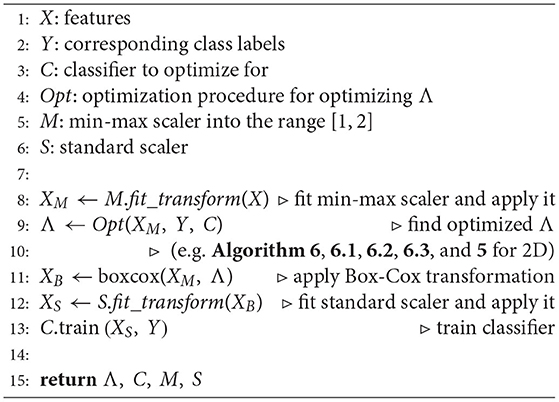
Algorithm 3 : fit_model(X, Y, C)

The prediction procedure is presented in Algorithm 4. It required the features, Λ, which was optimized during training, a fitted classifier, a fitted min-max scaler, and a fitted standard scaler. First, the method min-max scaled the data, then applied the Box-Cox transformation with the given Λ, then used standard scaling, and finally predicted the labels with the given classifier.

ALGORITHM 4

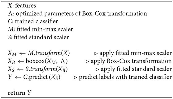
Algorithm 4 : prediction(X, Λ, C, M, S)

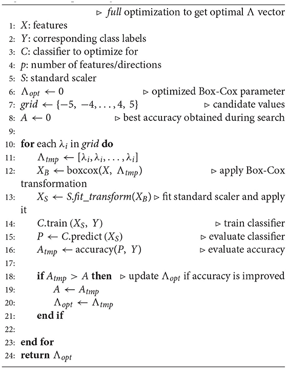
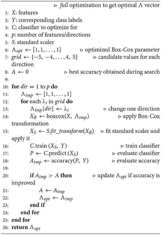
To follow the previously introduced notation in this paper, the optimization criteria L(·, ·) is defined as 1−ACC, which maximizes accuracy ACC by minimizing the 1−ACC optimizer. The first optimization procedure that was used in the training function was a grid search. This means that a set of possible values for every λ_i was specified. Then, the optimization tried all combinations. This was an exhaustive search and assuming model fitting and predicting as constant, it runs in polynomial time O(L^p) where L is the number of possible values and p is the number of features. Therefore, the grid search suffered from the curse of dimensionality. For example, trying 10 values for 10 features requires 10 billion evaluations. Therefore, this became quite infeasible. Nevertheless, it was used as a reference model for lower dimensional datasets. The pseudo-code for this method for the 2-dimensional case was given in Algorithm 5 and was directly used as optimization for training in Algorithm 3 in line 9.

ALGORITHM 5

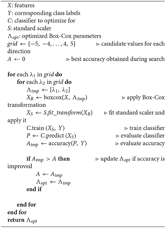
Algorithm 5 : 2D grid search(X, Y, C)

To solve the dimensionality problem of a grid search, we proposed an iterative optimization. First, an initial point, G∈ℝ^p, for Λ was specified. Then, starting from this point, all directions were fixed except for one. The not-fixed direction was optimized with a 1−dimensional grid search. Therefore, a set of candidate values for the search needed to be defined. Comparing the possible values and selecting the one that gave the highest improvement led to optimization in the first direction. Then, the next direction was unfixed and all other directions were fixed. Again, the best value was selected with a 1-dimensional grid search. This procedure was repeated until all directions were optimized once. This was referred to as one epoch. After that, the same procedure restarted with the previously optimized solution instead of the initial point G. The pseudocode for this iterative optimization was given in Algorithm 6 and will be referred to as Iterative grid search. It was directly used as an optimization procedure for training in Algorithm 3 in line 9. Assuming model fitting and predicting as constant, the advantage of this method is that it scaled linearly O(epochs·p·gridsize) in the number of features p, where gridsize denotes the number of points used for the 1-dimensional grid search. This procedure had three hyperparameters that influenced the result (initial starting point G, number of epochs, and the grid).

ALGORITHM 6

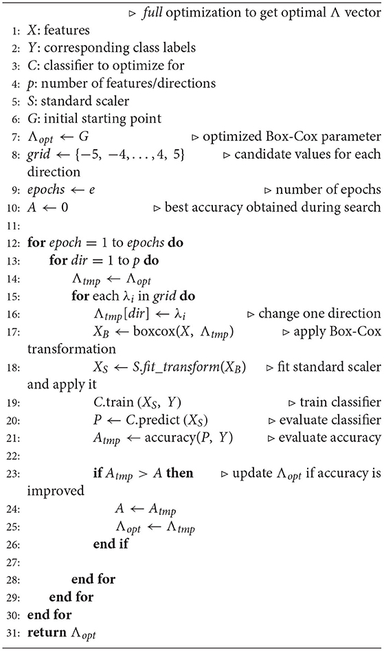
Algorithm 6 : Iterative grid search(X, Y, C)

Figure 3A shows why multiple epochs were beneficial. From the initial point G = [1, 1], first optimizing vertically in the λ₁ direction, and then horizontally in the λ₂ direction, gave an optimal value of 2 for Λ = [2, 2]. If another epoch, and thus another optimization in both directions, was added, the global optimal solution 3 at Λ = [3, 2] was obtained. Therefore, multiple epochs helped to find better optimization results.

FIGURE 3

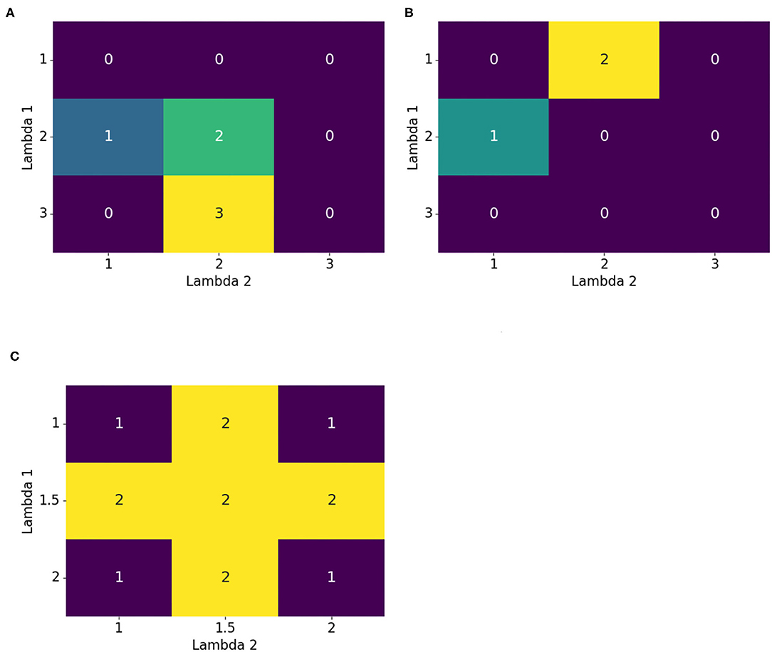
Figure 3. Motivations for improvements to the iterative method. Multiple epochs helped to further advance the optimization to the maximum. Multiple starting points and shuffling were introduced for escaping or avoiding a local maximum, and a finer grid provided the ability to explore hidden details. (A) Multiple epochs, (B) Multiple starting points and shuffling optimization order, and (C) Finer grid.

Another useful improvement was to restart the optimization with another initial point. Figure 3B illustrates this. Starting at G = [1, 1] and first optimizing vertically and then horizontally resulted in Λ_opt = [2, 1]. This cannot be further optimized with the given iterative method. Unfortunately, there was a better solution at Λ = [1, 2]. If, for example, the optimization started at G = [2, 2], the global optimal solution could be attained. Therefore, it was beneficial to restart the optimization procedure with multiple initial points. Corresponding modifications to the Iterative grid search optimization are found in Algorithm 6.1. It introduced the shift_epoch as a new hyperparameter that determined after how many epochs a new starting point G was generated.

ALGORITHM 6.1

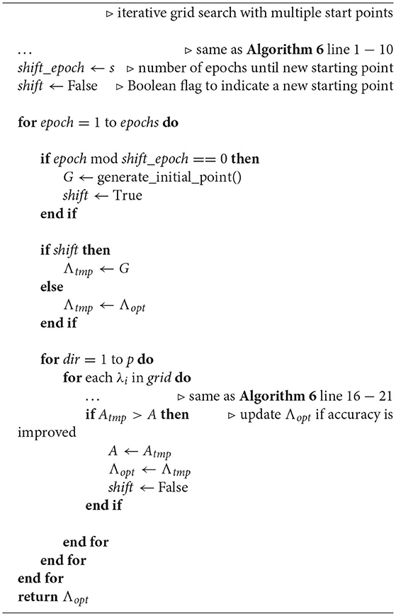
Algorithm 6.1: Shift(X, Y, C)

The previous problem could also be solved by changing the order of the optimization directions. So far, the directions have been optimized numerically; that is, first, λ₁ was optimized, then λ₂ and so on. Starting (in Figure 3B) again at the initial point G = [1, 1], instead of first optimizing in the vertical direction, optimization was done first in the horizontal direction. This directly found the global solution. Hence, shuffling the order of directions for optimization was also helpful. The corresponding changes to Iterative grid search are found in Algorithm 6.2. Again, there was a new hyperparameter shuffle_epoch that determined after how many epochs the optimization order got shuffled.

ALGORITHM 6.2

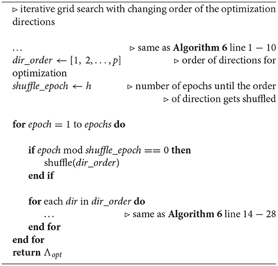
Algorithm 6.2 : Shuffle(X, Y, C)

Lastly, it might be possible to find a better solution if the grid search is denser. Figure 3C demonstrates this. If the grid only used integer values, then it was impossible to find one of the global optimal solutions = 2. Hence, the grid should be refined to 0.5 increments. Unfortunately, this doubled the computational demand. Another refinement may further improve the result but increase the computational demand even more. One solution to circumvent the increasing computational costs, was to use local refinement. This means that the grid became locally denser and smaller. Iterative grid search uses the same global grid for every 1-dimensional grid search (e.g. {−5, −4, …, 4, 5}). To get a finer grid, but with the same number of points, the grid needed to be attached locally to the current Λ_tmp. Since the number of grid points ought to remain the same and the grid became denser, it spanned a smaller range of values. For example, starting with the grid {−5, −4, …, 4, 5} and then doubling the resolution led to the following grid {−2.5, −2, …, 2, 2.5}. Both have the same number of points. Instead of testing globally, if any, λ_i∈{−5, −4, …, 4, 5} improved the result, the current optimal solution in this direction was used, and then the refined grid was attached to it. Therefore, it is tested, if any, λ_i∈{λ_{tmp, i}−2.5, λ_{tmp, i}−2, …, λ_{tmp, i}+2, λ_{tmp, i}+2.5} improved the accuracy. To take advantage of both global and local optimization, a global search was used at the beginning of the optimization to capture the full search domain. After some epochs, a local refinement was used to obtain a finer search space. With this modification, the computational cost remained the same. Additionally, it allowed for more and finer candidate values that could result in improvement. Incorporating this method into Iterative grid search is shown in Algorithm 6.3. As before, an additional hyperparameter finer_epoch was introduced to specify after how many epochs the grid was refined.

ALGORITHM 6.3

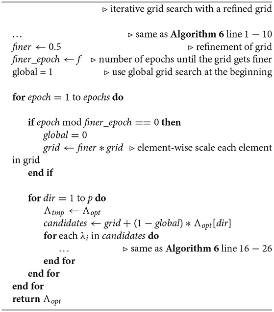
Algorithm 6.3 : Finer(X, Y, C)

Additionally, spherical and diagonal optimizations are given in Algorithms 7, 8. This was used for comparison with the proposed full optimization. These two methods were developed on classification accuracy like full optimization, rather than statistical evaluation (such as MLE or Fisher criterion) Bicego and Baldo (2016). The reason behind this approach is that the previous study showed that the Box-Cox parameter is classifier dependent.

ALGORITHM 7

Algorithm 7 : Spherical grid search(X, Y, C)

ALGORITHM 8

Algorithm 8 : Diagonal grid search(X, Y, C)

Results

Following the proposed optimization procedure was applied to different real-world datasets. The setup in Algorithm 2 was used which means that Algorithm 3 was used to train the model on the training data with the iterative optimization from Algorithm 6 and the corresponding improvements 6.1, 6.2, and 6.3. Then the performance was measured using the prediction function in Algorithm 4. The examined classifiers are given in Table 1. All results were measured with 10-fold stratified crossvalidation and 5 repetitions. To test the proposed method various settings for the hyperparameters were used. The setup is given in Table 4. Optimization in one direction was done evenly spaced over the interval [−5, 5] and gridsize corresponded to the number of grid points (e.g. gridsize of 11 gave the set {−5, −4, …, 4, 5} as candidate values). The Iterative grid search was just iterative optimization without any further improvements described in Algorithm 6. Shift, Shuffle, and Finer exclusively showed the influence of restarting the optimization with a new starting point given in Algorithm 6.1, changing the order of directions given in Algorithm 6.2, or refining the optimization grid given in Algorithm 6.3. Combined 1 and Combined 2 demonstrated how these improvements to the Iterative grid search optimization behaved in combination. The initial starting point, G∈ℝ^p, for the iterative optimization was chosen in each direction as the MLE. For comparison spherical and diagonal optimizations are given in Algorithms 7, 8 was also evaluated. Further traditional Box-Cox optimization of the log-likelihood function as in Box and Cox (1964) was applied column-wise. This approach maximized the Gaussianity of each column and is called MLE in the following tables.

TABLE 4

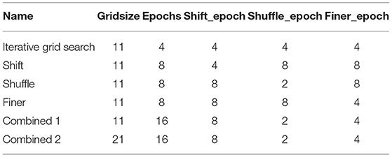
Table 4. Hyperparameter settings to test the iterative optimization on real-world data.

Sonar Dataset

The sonar dataset had 207 samples and 60 features. The labels were binary and indicated whether the sonar signal was reflected by a rock or metal. The measurements for the accuracy of the repeated cross-validation are given in Table 5. Additional measurements for the F1-score are given in the Appendix in Table B1.

TABLE 5

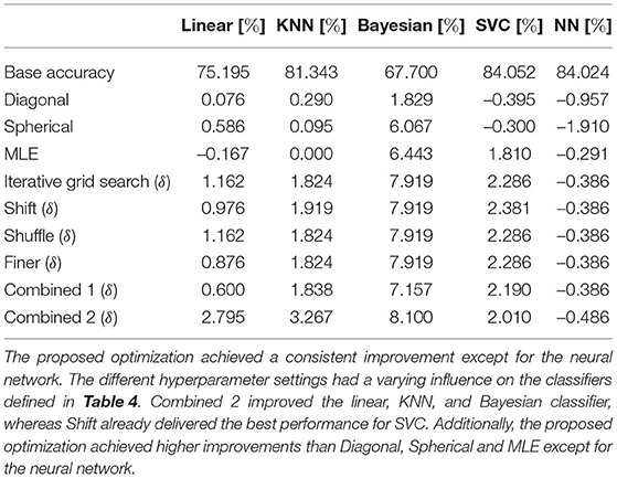
Table 5. Improvement δ in accuracy for different iterative optimization settings in the sonar dataset.

There was an improvement in accuracy for the proposed optimization for all classifiers except for the neural network. In particular, the Bayesian classifier improved on average by 7.8%. In contrast, the neural network decreased by −0.4% on average. The influence of the changes to the basic iterative optimization in Algorithm 6 with Shift, Shuffle, and Finer was observed for the linear and KNN classifiers. Shift restarted the optimization with a new initial point, and it seemed to decrease the accuracy for the linear classifier but slightly increased it for KNN. In contrast, shuffling the order of the directions during optimization did not result in an advantage for the classifier. Refining the grid after some epochs did not provide an increase in accuracy compared to basic iterative optimization. Combining these methods into one optimization sometimes decreased the performance (SVC) and sometimes increased the performance (KNN). Interestingly, the influence of the Combined 1 was better for the SVC and the neural network when compared to the Combined 2, which had a finer grid for Λ. The opposite was observed for the other classifiers. The Diagonal, Spherical, and MLE optimization performed worse than the proposed optimization except the MLE optimization lead to a smaller decrease in accuracy for the neural network. This behavior was also observed for the F1-score measurements given in Appendix in Table B1.

A 2-dimensional feature study was also performed. Two 2-dimensional datasets, Figures 4A,B, were created by extracting two random features from the sonar dataset. With a chi-square test, the ranks of the features were calculated. Then, a dataset with the two highest ranking features, Figure 4C and a dataset Figure 4D, with the third and fourth highest ranking features, were built. The performance of a grid search was measured and served as the baseline. This was done by using the training function in Algorithm 3 with 2D grid search from Algorithm 5 as optimization procedure and Algorithm 4 to create predictions. The grid search used the grid {−5, −4, …, 4, 5} in every direction. The datasets are shown in Figure 4, and the results for the accuracy are given in Table 6 and for the F1-scores in Appendix in Table B2.

FIGURE 4

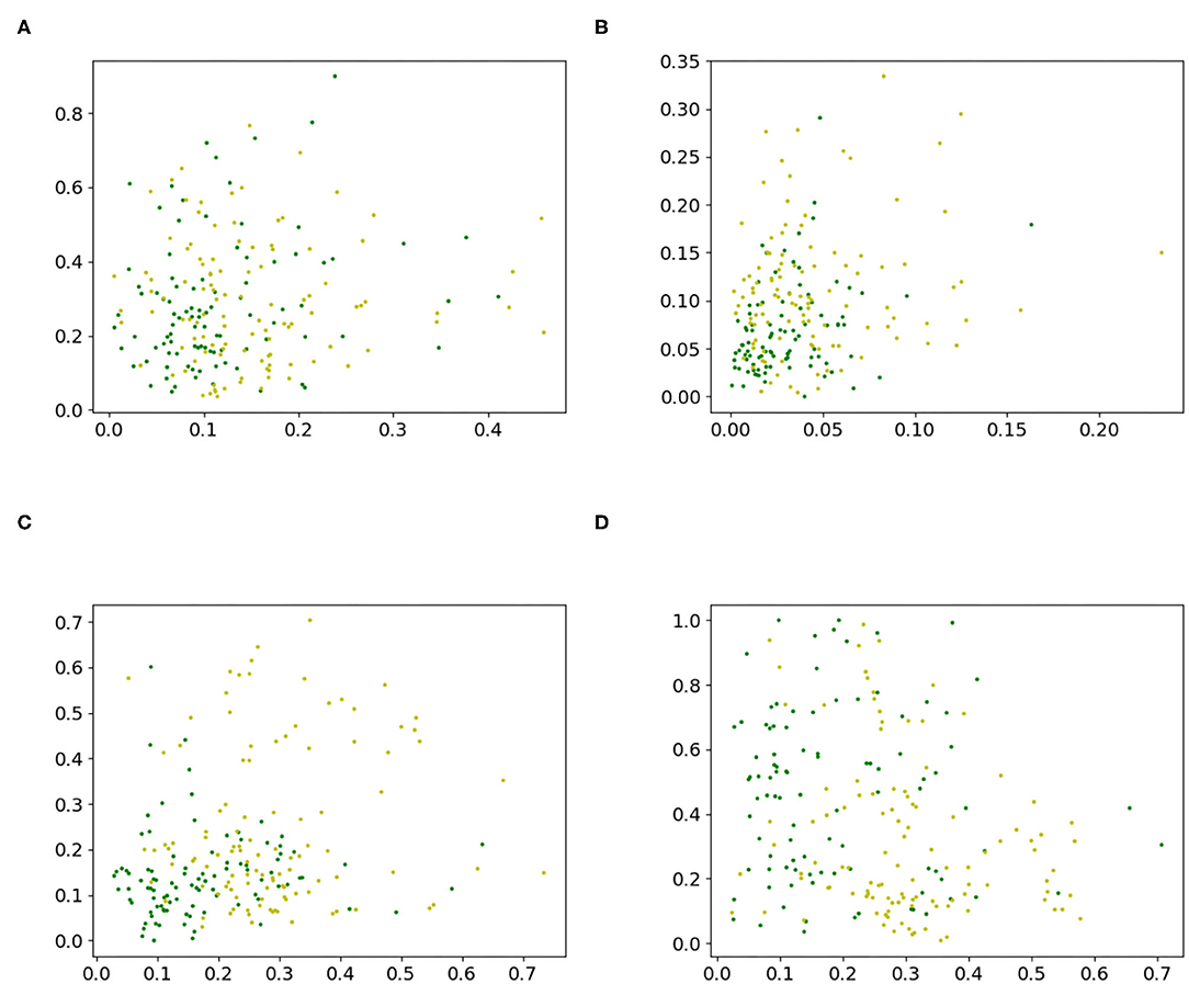
Figure 4. 2-D datasets extracted from the sonar dataset to compare proposed iterative optimization with a grid search. (A) features 8 and 41, (B) features 2 and 48, (C) features 11 and 45, and (D) features 12 and 36.

TABLE 6

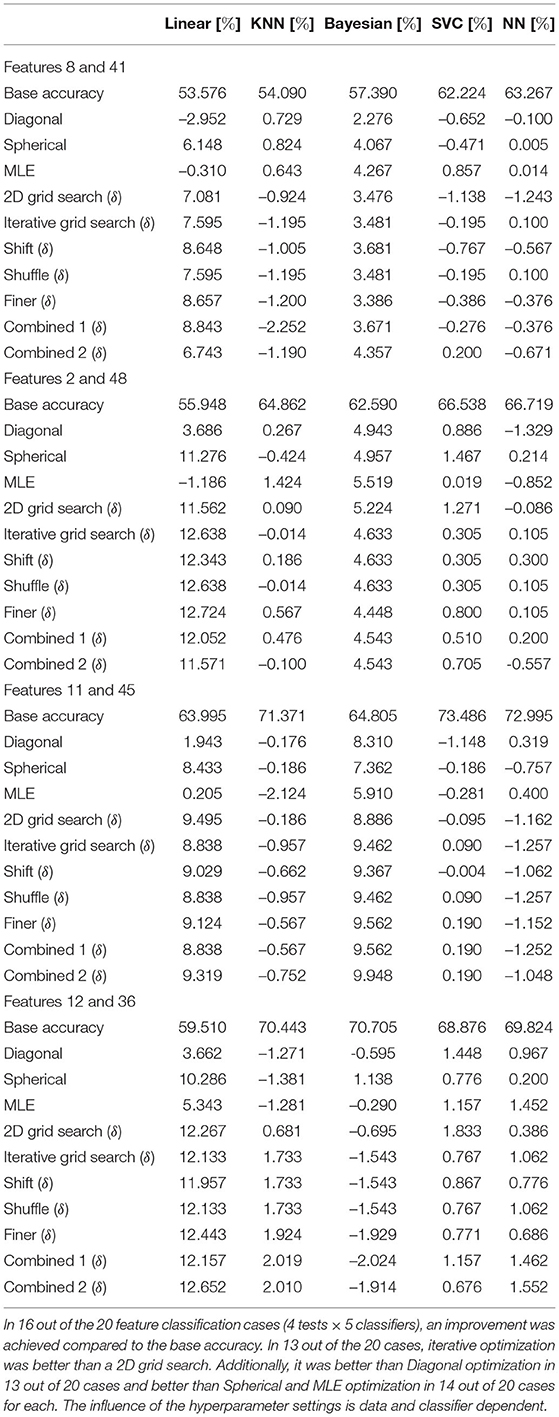
Table 6. Improvement δ in accuracy for different iterative optimization settings on 2-dimensional subsets of the sonar dataset.

The iterative method delivered an improvement of the base accuracy in 16 out of the 20 cases for at least one hyperparameter setting. Only the accuracy for the KNN classifier for features [8, 41] and [11, 45], the Bayesian classifier for features [12, 36], and the neural network for features [11, 45] could not be improved. Using the hyperparameter setting that resulted in the lowest loss for each case, the highest decrease in accuracy was only −1.543% (Bayesian classifier for features [12, 36]). In contrast, the best hyperparameter setting achieved a gain of 12.724% (linear classifier for features [12, 36]). Comparing the proposed iterative method to a grid search, the iterative optimization achieved better results for all classifiers for features [8, 41] for at least one hyperparameter setting except for the KNN classifier. Further, it provided gains for the linear, KNN, and neural network for features [2, 48], Bayesian, SVC, and neural network for features [11, 47], and linear, KNN and neural network for features [12, 36]. Hence, in 13 out of the 20 cases, iterative optimization resulted in better performance than 2D grid search. The gain in accuracy for the linear classifier was always positive. This also holds for the Bayesian classifier, except for features [12, 36]. The KNN classifier fluctuated around zero. Sometimes the iterative method cannot achieve any improvement for all tested hyperparameters setting (features [8, 41] and [11, 45]), and sometimes it was able to improve the result. For the SVC, there was always at least one hyperparameter choice that led to an improvement. The same can be observed for the neural network, except for features [11, 45]. Nevertheless, it resulted in a smaller loss of accuracy than grid search for the Shift, Finer, and Combined 2 cases. For all classifiers and datasets, there was often a set of hyperparameters that improved the result of the Iterative grid search optimization. Additionally, the influence of Shift and Finer compared to Iterative grid search was sometimes positive and sometimes negative. This varied between classifiers applied to the same dataset, for example, for features [8, 41] Finer increased the accuracy for the linear classifier but decreased the accuracy for the KNN classifier. Further, it varied between datasets for the same classifier, for example, the performance of the linear classifier for Shift increased for features [8, 41] but decreased for features [2, 48]. The same observation can be made for Combined 1 and Combined 2. Shuffle did not influence accuracy compared to Iterative grid search. The proposed method achieved better results than Diagonal optimization in 13 out of 20 cases. For Spherical and MLE optimization the results were better in 14 out of 20 cases for both. The measurements for the F1-score are given in Table 6. The proposed optimization achieved a better F1-score compared to the base accuracy in 12 out of 20 cases, compared to 2D grid search in 14 out of 20 cases, compared to Diagonal optimization in 13 out of 20 cases, compared to Spherical in 16 out of 20 cases and compared to MLE optimization in 12 out of 20 cases.

Breast Cancer Dataset

This dataset consisted of 569 samples and 30 features. It was a binary classification that distinguished between benign and malignant fine needle aspirate (FNA) samples. The influence of the iterative method on accuracy is given in Table 7. Additionally, measurements for the F1-score are given in the Appendix in Table C3.

TABLE 7

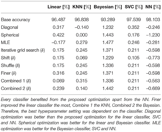
Table 7. Improvement δ in accuracy for different iterative optimization settings on the breast cancer dataset.

A similar observation to the sonar dataset was evident. There was an improvement for all classifiers except for the neural network. Again, the Bayesian classifier improved the most, and the influence of the different hyperparameter settings on the SVC was almost static. In comparison to Iterative grid search, Shift decreased the performance for all classifiers. Extending the Iterative grid search optimization with Shuffle had a small negative effect on the Bayesian classifier but did not change the accuracies of the other classifiers. Finer improved the results for the linear classifier but did not affect it for the other classifiers. Combined 1 improved the results of the KNN and neural network classifier compared to the Iterative grid search optimization. In contrast, Combined 2 only improved the neural network. The proposed optimization achieved an improvement of accuracy for the KNN and Bayesian classifier compared to Diagonal optimization, for the KNN, SVC, and NN compared to Spherical optimization, and for the linear classifier and KNN compared to the MLE optimization. The same was observed for the F1-scores in Appendix in Table C3 except that the proposed optimization achieved additionally an improvement for the linear classifier compared to the Diagonal optimization.

Again, a 2-dimensional feature study was performed. Two 2-dimensional datasets, Figures 5A,B, were created by randomly selecting two features from the breast cancer dataset. In addition, a dataset Figure 5C, with the two highest ranking features and a dataset, Figure 5D with the third and fourth highest ranking features were created by using the ranks of a chi-square test. The datasets are shown in Figure 5. The accuracy measurements are given in Table 8 and F1-scores in the Appendix in Table C4. A grid search with the grid {−5, −4, …, 4, 5} was also executed to obtain a baseline. Therefore, Algorithm 5 was used as an optimization procedure for the training method in Algorithms 3, 4 to create predictions.

FIGURE 5

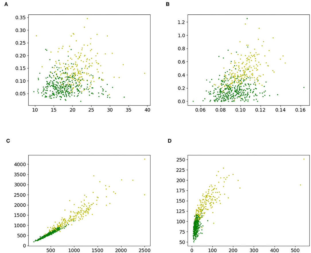
Figure 5. 2-D datasets extracted from the breast cancer dataset to compare proposed iterative optimization with a grid search. (A) Features 2 and 6, (B) features 5 and 27, (C) features 4 and 24, and (D) features 14 and 23.

TABLE 8

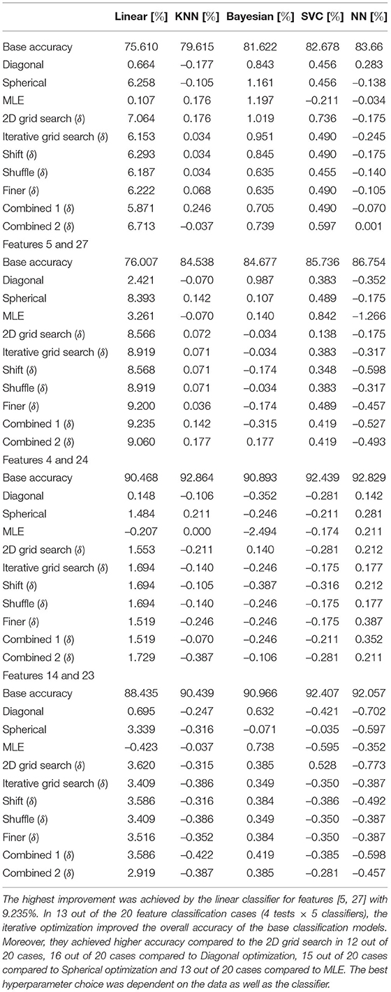
Table 8. Improvement δ in accuracy for different optimization settings on 2-dimensional subsets of the breast cancer dataset.

The iterative method resulted in an improvement of the base accuracy in 13 out of the 20 cases for at least one hyperparameter setting. The highest loss of the best hyperparameter setting was −0.387%. This was realized by the neural network for features [14, 23]. In contrast, the highest gain of 9.235% was achieved by the linear classifier for features [5, 27]. Compared to a grid search, the iterative method was able to achieve the same or better performance in 13 out of 20 cases for at least one hyperparameter setting. The linear classifier always benefited from the proposed optimization. The Bayesian classifier also achieved consistent improvements, except for features [4, 24]. The KNN classifier performance improved only in half of the cases (features [2, 6] and [5, 27]), as did that of the neural network (features [4, 24] and [2, 6]). As already observed in the experiment with the sonar dataset, Shift, and Finer both increased and decreased the performance compared to the Iterative grid search optimization. The influence varied from classifier to classifier and from dataset to dataset. For example, for features [2, 6] the linear classifier did benefit from the Shift, but the Bayesian classifier did not. In contrast, the linear classifier for features [5, 27] experienced a decrease in accuracy. Shuffle did not further influence the performance of the Iterative grid search method. Combined 1 and Combined 2 had varying influences depending on the classifier and the dataset. Compared to the proposed optimization, Diagonal optimization was worse in 16 out of 20 cases, Spherical optimization in 15 out of 20 cases, and MLE in 13 out of 20 cases. The F1-scores are given in the Appendix in Table C4 and comparable results were measured. The proposed optimization achieved a better score in 10 cases compared to the base accuracy, in 12 cases compared to 2D grid search, in 14 cases Diagonal optimization, in 15 cases compared to Spherical optimization, and in 13 cases compared to the MLE.

Discussion

With grid exploration, we have shown that the Box-Cox transformation is able to consistently improve the accuracy. This behavior was also observed by Bicego and Baldo (2016). According to their results, we have also demonstrated that optimization depends on the classifier. Further, we observed that full optimization leads to higher improvements. Therefore, suitable optimization is introduced. This method is further improved to be able to handle different problems during optimization. From two real-world datasets, we demonstrated that the proposed procedure is able to achieve improvements in accuracy and F1-score. Furthermore, we have shown that this optimization is superior to grid searches, diagonal, spherical, and MLE optimization in the majority of cases. We suspect that the iterative procedure introduces some implicit regularization. Grid search is likely to overfit the training data, whereas the iterative method might not be able to find a global solution on the training set and hence suffers less from overfitting. The proposed optimization also scales linearly with the ability to support finer grids. Real-world dataset studies have shown that the hyperparameter setting is dependent on the data itself and the classifier. Restarting the optimization with multiple starting points and refining the grid influenced the results. However, shuffling the optimization order did not have a meaningful impact.

The Box-Cox transformation is data-dependent. Hence, the optimal choice of λ varies, and we recommend using an appropriate optimization method. We have demonstrated that the optimization method should take the classifier into account. However, non-classifier-dependent optimization methods like MLE might also perform well. Therefore, the best approach to obtain the best Box-Cox transformation is to evaluate different optimization procedures and compare the results.

Conclusion

The impact of the Box-Cox transformation in classification tasks was examined. We extended the optimization of the parameters to a full dataset dependent problem and showed that this generalization improved the performance. An optimization procedure was proposed, successfully tested, and improvements up to 12% could be achieved.

In future work, an extensive application of the method to various datasets should be used to test the ability of the optimization. The influence of the hyperparameters should also be analyzed. Furthermore, the optimization could be improved by, for instance, replacing the 1-dimensional grid search with another 1-dimensional optimization. Although the Box-Cox transformation has been shown to increase the accuracy of a base classifier, it remains unclear whether it is also able to push the results of a classifier beyond state-of-the-art performance. Finally, the framework is designed with a general train-predict functionality that is often used in machine learning. Therefore, our method could also be applied to other tasks such as regression.

Data Availability Statement

The developed code and data are publicly available via the following link: github.com/Luca-Blum/Box-Cox-for-machine-learning.

Author Contributions

ME designed and led the study. LB, ME, and CM conceived the study. All authors approved final manuscript.

Conflict of Interest

The authors declare that the research was conducted in the absence of any commercial or financial relationships that could be construed as a potential conflict of interest.

Publisher's Note

All claims expressed in this article are solely those of the authors and do not necessarily represent those of their affiliated organizations, or those of the publisher, the editors and the reviewers. Any product that may be evaluated in this article, or claim that may be made by its manufacturer, is not guaranteed or endorsed by the publisher.

Supplementary Material

The Supplementary Material for this article can be found online at: https://www.frontiersin.org/articles/10.3389/frai.2022.877569/full#supplementary-material

References

Bicego, M., and Baldo, S. (2016). Properties of the box–cox transformation for pattern classification. Neurocomputing 218, 390–400. doi: 10.1016/j.neucom.2016.08.081

CrossRef Full Text | Google Scholar

Box, G. E. P., and Cox, D. R. (1964). An analysis of transformations. J. R. Stat. Soc. B 26, 211–252.

Google Scholar

Carroll, R. J., and Ruppert, D. (1985). Transformations in regression: a robust analysis. Technometrics 27, 1–12.

Google Scholar

Cheddad, A. (2020). On box-cox transformation for image normality and pattern classification. IEEE Access 8, 154975–154983. doi: 10.1109/access.2020.3018874

CrossRef Full Text | Google Scholar

Gao, Y., Zhang, T., and Yang, B. (2017). “Finding the best box-cox transformation in big data with meta-model learning: a case study on qct developer cloud,” in 2017 IEEE 4th International Conference on Cyber Security and Cloud Computing (CSCloud) (New York, NY: IEEE), 31–34.

Google Scholar

Kim, C., Storer, B. E., and Jeong, M. (1996). Note on box-cox transformation diagnostics. Technometrics 38, 178–180.

Google Scholar

Lawrance, A. J. (1988). Regression transformation diagnostics using local influence. J. Am. Stat. Assoc. 83, 1067–1072.

PubMed Abstract | Google Scholar

Liang, Y., Hussain, A., Abbott, D., Menon, C., Ward, R., and Elgendi, M. (2020). Impact of data transformation: an ecg heartbeat classification approach. Front. Digital Health 2, 53. doi: 10.3389/fdgth2020.610956

PubMed Abstract | CrossRef Full Text | Google Scholar

Pedregosa, F., Varoquaux, G., Gramfort, A., Michel, V., Thirion, B., Grisel, O., et al. (2011). Scikit-learn: machine learning in Python. J. Mach. Learn. Res. 12, 2825–2830.

Google Scholar

Sweeting, T. J. (1984). On the choice of prior distribution for the Box-Cox transformed linear model. Biometrika 71, 127–134.

Google Scholar

Vélez, J. I., Correa, J. C., and Marmolejo-Ramos, F. (2015). A new approach to the box–cox transformation. Front. Appl. Math. Stat. 1, 12. doi: 10.3389/fams.2015.00012

CrossRef Full Text | Google Scholar