Prediction of E. coli Concentrations in Agricultural Pond Waters: Application and Comparison of Machine Learning Algorithms

The microbial quality of irrigation water is an important issue as the use of contaminated waters has been linked to several foodborne outbreaks. To expedite microbial water quality determinations, many researchers estimate concentrations of the microbial contamination indicator Escherichia coli (E. coli) from the concentrations of physiochemical water quality parameters. However, these relationships are often non-linear and exhibit changes above or below certain threshold values. Machine learning (ML) algorithms have been shown to make accurate predictions in datasets with complex relationships. The purpose of this work was to evaluate several ML models for the prediction of E. coli in agricultural pond waters. Two ponds in Maryland were monitored from 2016 to 2018 during the irrigation season. E. coli concentrations along with 12 other water quality parameters were measured in water samples. The resulting datasets were used to predict E. coli using stochastic gradient boosting (SGB) machines, random forest (RF), support vector machines (SVM), and k-nearest neighbor (kNN) algorithms. The RF model provided the lowest RMSE value for predicted E. coli concentrations in both ponds in individual years and over consecutive years in almost all cases. For individual years, the RMSE of the predicted E. coli concentrations (log₁₀ CFU 100 ml⁻¹) ranged from 0.244 to 0.346 and 0.304 to 0.418 for Pond 1 and 2, respectively. For the 3-year datasets, these values were 0.334 and 0.381 for Pond 1 and 2, respectively. In most cases there was no significant difference (P > 0.05) between the RMSE of RF and other ML models when these RMSE were treated as statistics derived from 10-fold cross-validation performed with five repeats. Important E. coli predictors were turbidity, dissolved organic matter content, specific conductance, chlorophyll concentration, and temperature. Model predictive performance did not significantly differ when 5 predictors were used vs. 8 or 12, indicating that more tedious and costly measurements provide no substantial improvement in the predictive accuracy of the evaluated algorithms.

Introduction

Food safety is a fundamental public health concern which is threatened when waters with poor microbial quality are used for the irrigation of fresh produce. In the U.S. and around the world, regulatory or advisory thresholds on the microbial quality of irrigation waters are based on the concentrations of Escherichia coli (E. coli) measured in the water source (US Food and Drug Administration., 2015; Allende et al., 2018; Wen et al., 2020). Irrigation with water of substandard microbial quality has been implicated with foodborne outbreaks associated with the consumption of contaminated produce (Nygård et al., 2008; Kozak et al., 2013; Gelting et al., 2015). Additionally, it is known that pathogenic microorganisms transferred with irrigation water can internalize into crop tissues which extends their persistence and reduces the efficacy of post-harvest washing (Solomon et al., 2002; Martinez et al., 2015). Ensuring that water used for irrigation meets the recommended criteria is vital for protecting public health and reducing incidences of foodborne outbreaks.

Concentrations of fecal indicator organisms, primarily E. coli, are commonly used to characterize microbial water quality. Researchers have investigated the relationships between fecal microorganisms and water quality parameters such as dissolved oxygen, pH, turbidity, and nutrient levels with a goal of improving timeliness and predictability of microorganism concentrations in a water source (Francy et al., 2013; McEgan et al., 2013; Stocker et al., 2019). Such dependencies have varied considerably across studies. This may at least partially be explained by the complexity and non-linearity of relationships of fecal microorganisms with multiple water quality parameters, which in turn exhibit complex relationships.

Machine learning (ML) algorithms have been extensively shown to outperform traditional multivariate analyses in numerous aquatic ecology studies where the two analyses have been compared (Quetglas et al., 2011). The advantage of machine-learning methods is in their ability to mimic linear relationships between dependent and independent variables. Machine learning models are also able to assess associations and quantify predictability in the absence of the knowledge needed for developing process-based models (Thomas et al., 2018). Within the field of microbial water quality, several researchers have used ML algorithms to develop models which could be used to make rapid water quality determinations in rivers, streams, Great Lakes beaches, groundwater, drinking water wells, and water distribution systems (Brooks et al., 2016; Mohammed et al., 2018, 2021; Panidhapu et al., 2020; Tousi et al., 2021; Weller et al., 2021; White et al., 2021).

A large number of ML algorithms have been proposed and implemented in a variety of different research disciplines (Kuhn and Johnson, 2013). Common research goals are (a) to obtain an accurate predictive relationship between the predictors and target variables, and (b) to determine and rank the most influential predictors. By achieving these goals, researchers may be able to eliminate unimportant predictors from measurement programs which can potentially save a great deal of time and resources. The application of ML regressions in the field of microbial water quality is relatively new (Park et al., 2015; García-Alba et al., 2019; Stocker et al., 2019; Abimbola et al., 2020; Ballesté et al., 2020; Li et al., 2020; Belias et al., 2021; Wang et al., 2021). For agricultural waters, research into predicting E. coli concentrations using ML was done for streams (Weller et al., 2021), but so far no studies have utilized ML regressions to predict E. coli concentrations in agricultural irrigation ponds which serve as an important source of irrigation water across the United States and abroad.

The objectives of this work were (i) evaluate and compare the capabilities of several popular ML algorithms for predicting concentrations of E. coli from water quality parameters in irrigation ponds, and (ii) to determine the most influential predictors for the estimation of E. coli concentrations using a multiyear dataset.

Methods

Field Sites and Data Collection

Two working irrigation ponds in Maryland were sampled during the 2016–2018 growing seasons. Sampling typically occurred on a biweekly schedule between May and August. Specific details of the sampling procedures can be found in Pachepsky et al. (2018) and Stocker et al. (2021). Briefly, each pond was sampled in a grid-like pattern the maps of which are shown in Supplementary Figure 1. Pond P1 is located in central Maryland and provided irrigation water to the surrounding fruit fields. The northern part of the pond is surrounded by a forested area whereas the other two sides are covered by grasses or bushes. The fields around P1 received chemical fertilizers prior to planting each year in late March or early April.

Pond P2 is an excavated pond located on the University of Maryland's Wye Research and Education Center (WREC) which is located on Maryland's Eastern Shore. The pond receives water from a culvert at the northern end (location 12 on the map). The pond is surrounded by dense brush vegetation along the perimeter as well as by several trees planted further up from the banks. To the northern end of the pond is a small riparian area that surrounds an ephemeral creek while the southernmost portion has a wetland area that leads into the Wye River.

Along with each water sample that was collected, a YSI sonde was used to determine characteristics of the water quality in that sampling location. In 2016, a YSI MPS 556 (Yellow Springs Instruments, Yellow Springs Ohio) unit was used to measure dissolved oxygen (DO), pH (pH), specific conductance (SPC), and temperature (C) which were measured in-situ. At the laboratory, a Lamotte turbidimeter was used to measured turbidity (NTU) of the samples. In 2017, a YSI EXO 2 was used to measure all of the previously described water quality variables as well as the concentrations of chlorophyll (CHL), phycocyanin (PC), and fluorescent dissolved organic matter (f DOM). In 2018, the same YSI EXO 2 sonde was used but additional laboratory measurements were performed. These included ammonium (${\text{NH}}_4^{+}$), orthophosphate (${\text{PO}}_4^{3-}$), total nitrogen (TN), and total carbon (TC). Ammonium was measured using an ion-selective probe (CleanGrow, United Kingdom) which was calibrated prior to analysis which occurred on the same day as sample collected. Orthophosphate was run on a SEAL AQ300 discrete nutrient analyzer (SEAL Analytical, Mequon, Wisconsin). Total carbon and TN were analyzed on a Vario TOC cube (Elementar Hanau, Germany) using high temperature combustion and tandem TN_b and TC detectors.

E. coli enumeration was performed based on EPA method 1603 (US Environmental Protection Agency., 2005) which utilizes membrane filtration. Briefly, 100 ml of pond water was vacuum filtered through 0.45 μm membrane filters. Filters were then placed onto modified mTEC agar (BD Difco, Sparks, MD) and incubated for 2 h at 37°C and then 22 h at 44.5°C. After incubation, colonies that were purple in color were counted as E. coli. Each sample was duplicate plated and the resulting counts were then averaged.

Machine Learning Algorithms and Implementation

Several ML algorithms as well as a multiple linear regression (MLR) were compared in this work. The stochastic gradient boosting algorithm (SBG) builds the prediction model from an ensemble of weak models which in this case are decision trees (Friedman, 2002). Models are built in a step-wise fashion where at each step a weak model is fitted to a subsample of the training data drawn at random without replacement. The term “gradient boosting” comes from the fact the model is trying to minimize a loss function by tweaking parameters until a minimum value is reached. The R package “gbm” (Greenwell et al., 2020) was used develop SGB models. Parameters for the SGB algorithm are the number of trees (n.trees), the number of splits in the trees (interaction.depth), the learning rate (shrinkage), and minimum number of observations in terminal nodes of trees (n.minobsinnode).

The k-nearest neighbors (kNN) algorithm implements a non-parametric approach which computes distances from test datasets to the neighboring training datasets and uses these distances to determine the predicted value for the test dataset. The distances are computed from predictor values for training and test datasets. The number of neighbors (k) used for the prediction is the single parameter for this algorithm. A Euclidean distance measure was used to determine nearest neighbors. The “kknn” package (Schliep et al., 2016) was used to develop kNN models.

The support vector machines (SVM) algorithm finds the global minimum in the predictor (Cristianini and Shawe-Taylor, 2000). Support vector machines automatically select their model size and prevent overfitting by using special form of the regression cost function that balances accuracy and flexibility (Vapnik et al., 1995). Support vector machines neglects small errors which makes it robust and computationally treatable. It employs mapping to use linear regression while the relationship between original (not mapped) predictor and output variables is non-linear. The “kernlab” package (Karatzoglou et al., 2019) was used to run the SVM algorithm with a radial basis function kernel which has two control parameters. The γ parameter defines how far the influence of a single training example reaches and the parameter C controls the overfitting prevention.

The random forest (RF) algorithm creates predictions by generating many decision trees and combining their predictions in a weighted average giving the final prediction. The RF algorithm also has a built-in mechanism for preventing overfitting by random selection of inputs for the individual trees. As implemented in the ranger package (Wright and Ziegler, 2017), the algorithm includes three control parameters. The mtry parameter controls overfitting by determining the number of variables to randomly select at each split in the trees. The min.node.size parameter sets the minimum number of observations in a terminal node. The number of trees was kept at 500 to reduce computational intensity and because out-of-bag error did not appreciably change after this number of trees.

One of the outcomes of running RF algorithms is determining the most influential features that effect the model output. A random-forest based recursive feature elimination (RF-RFE) algorithm was applied to each dataset to determine the most influential predictors. The result of this procedure is to (i) find the subset of predictors with the minimum possible generalization error and (ii) to select the smallest possible subset of predictors which provide the optimal accuracy in model performance (Granitto et al., 2006). Within the algorithm, at each iteration feature importance is calculated based on the overall effect on the residual error and then the least important predictors are removed. The recursion is needed to address the problem that for some measures of relative importance, the results can change substantially over different subsets of the entire predictor list.

All ML algorithms as well as a MLR model were applied within the “caret” (classification and regression training) R package (Kuhn, 2008). This package contains functions that streamline training for complex ML regression and classification problems. The package facilitates the optimization and execution of ML algorithms and uses other R packages as functions for creating models. For each of the above-listed ML algorithms, we used the “caret” package to perform repeated cross-validation when fitting the ML models to the datasets. A default 10-fold cross-validation was performed with five repeats and then the results were averaged. The “caret” package was also applied to perform the recursive feature elimination. Algorithm tuning was performed during cross-validation and tuning was performed to minimize the average root mean squared error $\overline{RMSE}.$ The “caret” package contains a grid search function for control parameter tuning which was utilized in this study. The optimal control parameters as well as most influential variables were identified during cross-validation.

Comparison of Algorithm Performance Metrics

The average root mean square error $\overline{RMSE}$, coefficient of determination $\overline{R^2}$, and mean absolute error $\overline{MAE}$ were the metrics used to evaluate algorithm performance in this study. Averaging of RMSE, R² and MAE was done across 50 values of those statistics obtained for all cross-validation folds and repeats. The probability of the averages being the same for a pair of algorithms was determined from the corrected Student statistics t_c:

$\begin{array}{ll}{t}_{c,RMSE}=\frac{{\overline{RMSE}}_1-{\overline{RMSE}}_2}{\sqrt{h{\sigma }_{RMS{E}_1-RMS{E}_2}^2}};t_{c,MAE}=\frac{{\overline{MAE}}_1-{\overline{MAE}}_2}{\sqrt{h{\sigma }_{MA{E}_1-MA{E}_2}^2}};& (1)\end{array}$

$\begin{array}{l}{t}_{c,R^2}=\frac{\overline{R_1^2}-\overline{R_2^2}}{\sqrt{h{\sigma }_{R_1^2-R_2^2}^2}};\end{array}$

where subscripts “1” and “2” refer to the first and the second compared algorithms, ${\sigma }_{RMS{E}_1-RMS{E}_2}^2$, ${\sigma }_{MA{E}_1-MA{E}_2}^2$, and ${\sigma }_{R_1^2-R_2^2}^2$ are variances of differences between the values of RMSE, MAE, and R², respectively, obtained for the same fold and repeat, h is the variance correction term proposed by Bouckaert and Frank (2004) to account for the fact that that values of the metrics in the 50 individual random samples are not independent as they are obtained by the random subsampling of the same dataset. The value of h is determined as

$\begin{array}{ll}h=\frac{1}{k·r}+\frac{n_{testing}}{n_{training}}& (2)\end{array}$

where k is the number of folds and r is the number of repeats, n_training instances are used for training, and the remaining n_testing instances for testing in each of runs. The t_c statistics in (1) have the Student t distribution with k·r – 1 degrees of freedom. The value of the ratio n_testing/n_training was 0.1 in this work as recommended by Bouckaert and Frank (2004). Having the value and knowing the distribution of t_c, one can estimate the probability of the differences between the average metrics from two models being equal to zero. Bouckaert and Frank (2004) referred to this test statistic as the “corrected repeated k-fold cv test.”

Normalized root-mean-square-error (NRMSE) and mean absolute error (NMAE) were also computed by dividing the $\overline{RMSE}$ and the $\overline{MAE}$, respectively, by the range of E. coli concentrations (e.g., maximum–minimum concentration) and then multiplying by 100 for each year and predictor set. NRMSE and NMAE show the percentage of algorithm error relative to the spread of data.

Data Preprocessing and Analysis

Escherichia coli count data was log-transformed prior to statistical analysis. All observations of 0 CFU 100 ml⁻¹ were assigned a value of 0.5 to facilitate the log-transformation (US Environmental Protection Agency., 2005). Rows with missing values were removed prior to analysis. Data was not normalized or standardized before analysis. Preliminary findings showed that these operations did not substantially affect algorithms performance and in many cases resulted in poorer predictions.

To examine model performance and variable importance using different combinations of predictors, we created three different predictor sets. These included set A which is DO, pH, SPC, NTU, and C, set AB which is set A plus f DOM, PC, and CHL, and set ABC which is set AB plus ${\text{PO}}_4^{3-}$, ${\text{NH}}_4^{+}$, TN, and TC. Models with the Set A were developed for the individual years 2016 to 2018 and the combined 3-year dataset. Models with Set AB predictors were developed for 2017 and 2018, and models with the set ABC predictor were built only for 2018 where all 12 of the parameters were measured.

A separate study was performed to evaluate the models developed with the combined P1 and P2 datasets as opposed to models developed with separate P1 and P2 datasets. Only the predictor set A was evaluated in this exercise because these predictors were present in all years of observations and across ponds. The combined dataset was modeled with and without the introduction of a categorical variable “site” that labeled the data from different ponds.

Results

Summary of Monitoring Data

The P1 2016A, 2017A, and 2018A datasets contained 50, 126, and 138 samples, respectively, after row removal due to missing values. The P1 2017AB and 2018 AB were 126 and 138 samples, respectively, while the 2018ABC dataset was 92 samples after row removal. For P2, the sample set sizes were 97, 148, and 202 samples for 2016A, 2017A, and 2018A, respectively and the 2017AB and 2018AB had the same dimensions as the A scenario set. The P2 2018ABC dataset had 202 samples.

Escherichia coli and other water quality variable concentration averages and standard errors are shown in Supplementary Table 1. The two ponds contained similar concentration ranges of E. coli in general although the P1 2017 dataset year contained consistently higher concentrations. The 2016 datasets for each pond contained higher amounts of missing values of E. coli concentrations compared to the 2017 and 2018 datasets which had relatively few (<5%).

Values of most of the water quality parameters were similar between ponds with a few exceptions. Pond 2 in 2017 and 2018 had elevated DO concentrations compared to other instances. CHL and PC were also several times higher in P2 than in P1 in 2017 and 2018. The 2016 NTU concentrations at P2 were considerably higher than in other cases. Orthophosphate concentrations were about 16.5 times greater at P2 than in P1 in 2018. However, P1 had an average ${\text{NH}}_4^{+}$ concentration which was about three times greater than in P2. Average SPC values varied between 142.59 and 166.95 across the two ponds. Average f DOM values were higher in P2 in 2017 and 2018 than P1 for each corresponding year.

Evaluation of Machine Learning Algorithm Performance

The $\overline{RMSE}$ values and standard errors of RMSE are presented in Table 1. As expected, the MLR performed substantially worse than the ML algorithms for both ponds and for all years and predictor sets. The differences between the performance of the ML algorithms were less substantial. Overall, the differences among average SVM, RF, and SGB $\overline{RMSE}$ for the same ponds and years were <10%. The kNN demonstrated relatively larger spread of differences between its RMSE and $\overline{RMSE}$ of other ML algorithms and the range of those differences was from 1.5 to 24.9%.

TABLE 1

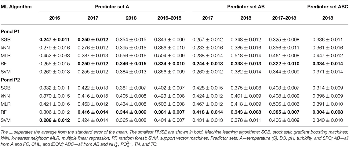
Table 1. Average root-mean-squared errors (RMSE) of logarithms of E. coli concentrations predicted with four machine learning algorithms and multiple linear regression.

Random Forest as the Best-Performing Algorithm

The RF algorithm provided the smallest $\overline{RMSE}$ value in 88% of cases. Only in 2016, the SGB and SVM algorithms, on average, provided lower RMSE values for P1 and P2, respectively. The SGB algorithm provided the second smallest $\overline{RMSE}$ in 75% of cases. Probabilities of $\overline{RMSE}$ being equal for RF and other algorithms are shown in Figure 1. The probability ranges differed between the ponds and among algorithms. Whereas the probabilities of equal $\overline{RMSE}$ for SGB and RF were high for Pond 1, Pond 2 had a greater spread of probabilities that were generally lower. Similarly, the range of probabilities of equality of $\overline{RMSE}$ for RF and kNN was much wider for Pond 2 compared with Pond 1. Probabilities of equal $\overline{RMSE}$ for RF and SVM were relatively high in both ponds. Ranges of those probabilities were similar in both ponds, unlike with other algorithms. The two significant differences in model performance occurred between the RF and kNN algorithms with the 2018 A (P < 0.043) and the 2018 ABC (P < 0.001) P2 datasets.

FIGURE 1

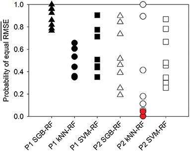
Figure 1. Probabilities for the mean RMSE value to be the same in the RF and other ML applications based on the corrected t-statistic. Symbols in red show statistical significance.

Interannual Differences in Algorithm Performance

Probabilities of the absence of differences in $\overline{RMSE}$ for pairs of years varied by year, algorithm, and pond (Supplementary Table 2). Comparisons between 2016 and 2017 performance were not significant in the P1 dataset. For P2, the SVM, RF, and SGB algorithms performed significantly better on the 2017 than the 2016 set. The 2017 predictor A set showed significantly better performance than the 2018 A set in P1 but was not found to significantly differ for any model in P2. Between the 2016 and 2018 predictor A sets, the SGB, kNN, and SVM algorithms performed significantly better for the 2016 dataset than for the 2018 dataset whereas the performance, while better for RF and MLR in 2016, did not significantly differ. The MLR model was the only model at P2 which showed significantly better performance in 2016 when compared to 2018.

Multiannual Algorithm Performance

When ML algorithms were applied to the three-year dataset from P1 with the predictor set A, the $\overline{RMSE}$ appeared to lie between the maximum and minimum $\overline{RMSE}$ obtained for individual years for the same pond and predictor set. For P2 and predictor set A, the $\overline{RMSE}$ of the three-year dataset were slightly higher than the largest of the individual year $\overline{RMSE}$. A similar pattern was observed with the predictor set AB and the 2-year dataset. The $\overline{RMSE}$ for P1 was between the $\overline{RMSE}$s of individual years, whereas with P2 data, the $\overline{RMSE}$ of individual years were smaller than the $\overline{RMSE}$ of the 2-year dataset.

Effect of the Predictor Set Expansion

Expanding the predictor set size from A to AB in the 2017 resulted in a slight increase of $\overline{RMSE}$ in most cases with the one exception being for the RF model in P1. Transition from A to AB and then to ABC predictor sets generally led to the decrease of $\overline{RMSE}$ (Figure 2). However, in some cases there was effectively no difference (i.e., RF in P1 between AB and ABC and kNN between all sets in P2). In P1, there was a gradual decrease in RMSE with increased number of predictors whereas for P2 the largest RMSE decreases were between AB and ABC with kNN being the exception. In all cases the 12-predictor ABC set showed the best performance for all ML algorithms at both ponds.

FIGURE 2

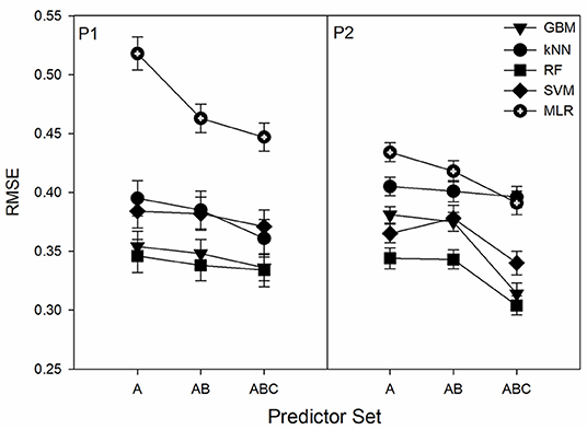
Figure 2. Dependence of the root-mean-squared error (RMSE) on the predictor set size. Predictor sets have 5, 8, and 12 predictors for A, AB, and ABC, respectively. Displayed results are from the 2018 datasets.

Other Metrics of Algorithm Performance

The differences between algorithm performance measured with mean absolute error (MAE) and the determination coefficient (R²) were similar to the differences found with RMSE values (Supplementary Tables 3, 4). However, in a few instances the model with the best performance changed when analyzing different metrics. For example, the SGB model provided the best performance in the 2018 ABC predictor set in P1 and the kNN provided the best result for the 2016–2018 predictor set A for P2 when using MAE as a metric. These two were predicted most accurately by the RF model when RMSE is used. Similarly, the SGB model in P1 2017–2018 AB predictor set in P1 provided the highest R²-value and the kNN model was best in the 2017 A predictor set in P2 whereas both were predicted best by the RF model when using RMSE.

The RF algorithm provided either the best (12 cases) or the second best (4 cases) value of the average MAE. The SGB and SVM algorithms were the closest to the RF (Supplementary Table 3). Similar to the results comparing RMSE, the 2016 and 2017A and AB sets were predicted with the lowest errors according to average MAE and errors were generally lower with P1 than P2. The only significant differences in ML model performances using the MAE metric was between the RF and kNN in the P2 2018 ABC dataset (P = 0.004) (Supplementary Figure 2). Based on R²-values, the RF model was preferred in 12 of 16 cases with it being second in two cases and tied with the SGB model in two cases (Supplementary Table 4). Interestingly, R²-values for the 2017 A and AB sets were the lowest across models despite this year having the smallest average RMSE and MAE values. Similar to results with RMSE and MAE, kNN was the only ML model to perform significantly worse (P = 0.003) than the RF model which occurred for the 2017–2018 AB dataset (Supplementary Figure 3).

Normalized RMSE and MAE were calculated for all years and predictor sets for both ponds (Supplementary Tables 5, 6). The preferred algorithm did not change from those presented in Table 1 and Supplementary Table 2 for values of RMSE and MAE, since for a given dataset, RMSE and MAE values from all algorithm were divided by the same value. The percentages of the errors as shown by examination of NRMSE values (Supplementary Table 5) for the ML algorithms were generally around 10 % of the data range for the P1 2016A, 2017A, 2016–2018A, and 2017AB datasets. The P1 2018A, AB, and ABC datasets contained higher errors which were between 10 and 20%. The MLR algorithm provided consistently higher errors which were typically in the range of 15–20% except for the 2017 datasets which had <10% error. P2 contained greater relative error (15–20%) than the P1 datasets with the exception being the 2018A, AB, and ABC data in which errors were in the same range between ponds. Values of NMAE were consistently lower than those of NRMSE and were in the range of 5.2% to (RF P1 2017A) to 15.5% (MLR P2 2018 A).

Algorithm Performance for the Combined Pond 1 and Pond 2 Datasets

Results of combining the P1 and P2 datasets are shown in Supplementary Table 6. The SVM algorithm performed the best in terms of values of RMSE, R², and MAE in the combined 2016 dataset whereas the RF algorithm showed the best performance in the 2017, 2018, and 2016–2018 datasets. The algorithm performance for the combined P1 and P2 dataset was never better than the performance of both ponds run individually for certain years but was typically higher than one pond and lower for the other (Table 1; Supplementary Tables 3–5). Including “site” as a categorical input generally improved the performance of the combined P1/P2 datasets across years (Supplementary Table 7).

Recursive Feature Elimination

In almost all scenarios the RF model was shown to provide the best $\overline{RMSE}$ values when compared to the other models. For this reason, a recursive feature elimination in “caret” was performed using the RF model to determine and rank the most important features for each pond and by year. Supplementary Figure 4 shows the reduction in RMSE values for the RF models for each year. Examination of the graph shows that in most cases the models do not greatly benefit from more than five predictors but the specific predictors varied by pond and year. The predictor importance order for each year from the RF-RFE was recorded and each variable received a numeric value corresponding to the overall ranking (Table 2). In this way, the variables with the lowest scores corresponded to being picked as consistently most important.

TABLE 2

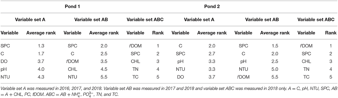
Table 2. The top five important variable as determined by the recursive feature selection algorithm in caret with Random Forests.

Within the various predictor set scenarios, there were some parameters that were consistently highly ranked as important features. These included SPC, C, f DOM, CHL, and NTU. All other parameters showed largely inconsistent ranking. While SPC was consistently ranked in the top two variables for all scenarios, temperature was as well for variable sets A and AB but was ranked poorly in the ABC datasets. The PC-value was consistently ranked low in the datasets that contained this parameter. Similarly, ${\text{NH}}_4^{+}$ and ${\text{PO}}_4^{3-}$, the only ionic nutrients measured in the study were also ranked low in the ABC set. Conversely, TN and TC were ranked fourth and fifth important in both ponds in the 2018 datasets. Interestingly, the 2018 ABC parameter sets had identical rankings of the five top important features and overall similar rankings of the remaining seven parameters.

Discussion

While model performance generally did not significantly differ, the RF model was found to provide consistently better performance than any of the other models evaluated. Several publications focusing on ML model evaluation specifically for microbial water quality purposes have reached similar conclusions (Avila et al., 2018; Chen et al., 2020; Weller et al., 2021). The SGB model was found to provide the second-best performance across all three metrics from all datasets. In several empirical ML comparison studies, it has been stated that SGB models usually outperform RF models (Maclin and Opitz, 1997; Caruana and Niculescu-Mizil, 2006; Hastie et al., 2009) but other studies report the opposite (Bauer and Kohavi, 1999; Manchanda et al., 2007; Khoshgoftaar et al., 2010). Therefore, the choice of “the best” model may be dataset-dependent which to some degree was evident in the results of this work (Table 1; Supplementary Tables 3, 4). Also, the performance of both models is dependent on how they are tuned. SGB are considered harder to tune than RF models, contain greater sensitivity of tuning parameters with regard to the output, and have a greater number of tuning parameters (Freeman et al., 2016). Both RF and SGB algorithms are tree-based but the SGB algorithm incorporates a boosting procedure whereby model fitting is additive and each new tree is fit to the residuals of the previous tree with the goal of minimizing the most egregious errors according to a specific loss function such as MSE. Because SGBs are additive, they are more susceptible to over- or underfitting which the RF model is robust to because the individual trees are independent and are averaged to create the forest. Lastly, when bagging (RF) and boosting (SGB) type algorithms have been compared, bagging has been described to provide better results when datasets are noisy or there are class imbalances (Maclin and Opitz, 1997; Khoshgoftaar et al., 2010).

The performance of the SVM and kNN algorithms was generally poorer than the RF and SGB algorithms (Table 1) but in most cases the performance did not significantly differ (Figure 1). One possibility is that both SVM and kNN algorithms have been reported to not handle missing values, near-zero variance predictors, or noisy data as well as RF or SGB algorithms (Kuhn and Johnson, 2013). The SVM algorithm typically provided lower RMSE than the kNN algorithm and this may be because SVM is robust to outliers especially when non-linear kernels are used. The RBF kernel was used in this study because it provided substantially better results than the linear or polynomial kernels (data not shown) which was also reported in the work by Weller et al. (2021) who used ML algorithms for the prediction of E. coli in NY streams. Several other water quality studies have also reported better performance of SVM than kNN when the two have been compared (Modaresi and Araghinejad, 2014; Danades et al., 2016; Babbar and Babbar, 2017; Prakash et al., 2018; Chen et al., 2020). Finally, the kNN has been reported to not perform well with high dimensional or highly scattered datasets which is why centering and scaling is recommended. However, in our work, this pre-processing procedure did not affect results but may explain why SVM is preferred in other water quality datasets.

Different performance metrics in general agreed with each other, but in some cases contradicted. For example, while all algorithms showed the best $\overline{RMSE}$ on the 2017 P1 dataset (Table 1), this year was ranked the worst predicted by the R² metric (Supplementary Table 4). This is caused by the distribution of observed and predicted data along a 1:1 line. This example highlights the importance on the choice of performance metric reported in algorithm evaluation studies and the advantage of using multiple performance metrics.

We compared only five different algorithms in this study which were chosen due their popularity, but many more ML algorithms and their modifications exist and can be tested for regression-type application (Kuhn, 2008; Kuhn and Johnson, 2013; Weller et al., 2021). We chose not to run artificial neural networks (ANN) due to constraints of the dataset dimensions but other researchers have found success in applying ANN algorithms in the field of microbial water quality (Motamarri and Boccelli, 2012; Buyrukoglu et al., 2021). Other promising algorithms for water quality determinations include those founded in Bayesian statistical methods such as Naïve Bayes or Bayesian Belief Networks (Avila et al., 2018; Panidhapu et al., 2020) and the use of ensemble or model stacking methods (Buyrukoglu et al., 2021).

Several predictor variables emerged as consistently important for both ponds and across years of observations. These included f DOM, SPC, C, and CHL, and NTU. Positive relationships between dissolved organic matter (f DOM) and concentrations of planktonic fecal bacteria in water have been reported (Rincon and Pulgarin, 2004; Bouteleux et al., 2005). The relationship is likely governed by the presence of suspended organic substances which may promote the growth and survival of E. coli in the present study by providing nutrients, an attachment surface, and decreasing direct cellular photo-inactivation (Rincon and Pulgarin, 2004; Garcia-Armisen and Servais, 2009; Maraccini et al., 2016; KatarŽyte et al., 2018).

In both ponds and in every year NTU was positively correlated with E. coli concentrations (data not shown). Positive associations of fecal bacteria and NTU have been previously presented (Francy et al., 2013; Partyka et al., 2018; Weller et al., 2020) and can also be related to the level of suspended particulates which have been shown to enhance E. coli survival in water (KatarŽyte et al., 2018). Additionally, elevated NTU levels may indicate recent disruption of bottom sediments either by bioturbation or runoff-related mixing which results in the resuspension of fecal bacteria contained in sediments (Cho et al., 2010; Stocker et al., 2016).

The presence of CHL in the lists of most important predictors apparently reflects mutualistic relationships between algae and E. coli have been reported and attributed to solar shielding as well algae providing a source of labile organic nutrients which promote bacterial persistence (Englebert et al., 2008; Vogeleer et al., 2014). On average in both ponds, when chlorophyll-a (CHL-a) levels were higher, E. coli concentrations were lower (Supplementary Table 1). There may exist a threshold level at which there is a mutualistic relationship between E. coli and algae and above this level there exists competition (Ansa et al., 2011).

The concentrations of SPC were determined as most important in the largest number of cases in the study. The concentrations of SPC in water are proportional to the ion concentrations present. Ionic nutrient concentrations in water have often shown positive relationships with the concentrations of E. coli present (Lim and Flint, 1989; Ozkanca, 1993; Shelton et al., 2014). Recent research has also demonstrated that E. coli survival rates in freshwater increase with conductivity by way of reducing osmotic stress and improving membrane stability but can be detrimental above certain levels (DeVilbiss et al., 2021). Runoff reaching waterways may either have a dilutional effect and lower water conductance or increase it (Baker et al., 2019). Rapid changes in SPC may be used as an indicator of when influent such as runoff or precipitation has reached water sources and thus may provide good indication of when E. coli concentrations can be expected to change within a waterbody.

Temperature effects on E. coli persistence in the environment are perhaps the most well-documented of any other variables in the literature but may also be the most inconsistent. Numerous review and meta-analysis articles indicate E. coli persistence is negatively influenced by higher temperatures (Blaustein et al., 2013; Stocker et al., 2014; Cho et al., 2016). However, others have reported positive relationships (Truchado et al., 2018) while some have reported inconsistent direction of the relationship when multiple sites were included in the same study (Francy et al., 2013; McEgan et al., 2013). These diverse dependencies reveal the complexity of the relationships between E. coli and the predictors which govern the aquatic habitat and affect survival. Ultimately, ML algorithms are expected to handle the complex interactions and non-linear relationships better than traditional regression models in aquatic studies (Quetglas et al., 2011; Weller et al., 2021).

Through additional scenario testing (Table 2; Supplementary Tables 3, 4) it was discovered that model performances did not substantially change when the 2017 and 2018 datasets were held at a lower number of predictors. This indicates while parameters introduced in later years of the study were found to be at times more important, the core 5 predictors utilized in 2016A, 2017A, and 2018A predictor sets (C, SPC, NTU, DO, and pH) were found to be largely suitable for predicting E. coli concentrations in agricultural pond waters. This finding is of special interest as each additional predictor introduces additional burden on water quality characterization program. Additionally, results of this study indicate that E. coli concentrations in irrigation ponds may be “now casted” by using relatively cheap deployable on-line sensor suites that are used for continuous monitoring. It must be acknowledged that this study utilized measurements of a total of 12 predictors. Many additional predictors exist (e.g., ORP, total suspended solids, or various nutrient concentrations such as nitrate or ammonia) which may further improve the predictive performance of the ML algorithms or lead to the creation of similar simple and effective sets of variables as those identified in this study.

We realize that the effect of redundancy of predictors was not fully elucidated in this work. There exist multiple suggestions on redundancy removal as a preprocessing step of regressions using correlations between predictors, variance inflation estimation, or principal component analysis as a basis for the removal of covarying predictors. Multiple methods are suggested in the literature to reduce the effects of the input reduction on variable importance determinations (Bøvelstad et al., 2007). These methods tend to increase the reliability of the regression results (more data per coefficient), but at the same time, they may change the perception of the relative importance of input variables (Ransom et al., 2019). Applying these methods to several ML algorithms and assessing results presents an interesting research avenue. In this work, we limited the study by analyzing correlations between inputs. As expected, the only strong correlations were found between DO and pH (data not shown). The most likely mechanism for the observed co-linearity is photosynthetic activity in the ponds which consumes dissolved CO₂ (raising pH) and releases DO (raising DO). We cannot exclude the effect of this correlation on the occurrence and position of DO and pH in lists of important inputs.

The algorithm performance for the combined P1 and P2 dataset was never better than the performance of both ponds run individually for certain years but was typically higher than one pond and lower for the other (Table 1; Supplementary Tables 3–5). Explanations for this may be site-specific responses of E. coli concentrations to differences in predictor levels in each pond which may in some cases be similar and in others dissimilar. For example, P2 had elevated levels of the photosynthetic pigments PC and CHL compared to P1. Similarly, DO and pH levels in P2 were typically higher in P2 than in P1 (Supplementary Table 1). It is therefore possible that there were different extents to the effects of these predictor levels on E. coli concentrations which were unique for each pond. If monitoring datasets are available for multiple water bodies, one can pool these datasets together and compare the performance between site-specific models and those developed using pooled datasets across locations. Alternatively, one may use “site” as categorical variable input which may preserve site-specific interactions between E. coli and predictors within a larger model. Indeed, in the present study, adding “site” (e.g., Pond 1 or Pond 2) generally improved the performance of all algorithms on the P1/P2 combined datasets (Supplementary Tables 5, 6).

The results of this work were gathered by studying only two irrigation ponds both in the state of Maryland and as such the scope of inference is limited. However, in the literature there is a lack of information regarding E. coli and water quality dynamics in irrigation sources let alone those involving ML algorithms. The current study suggests a framework for using ML algorithms for irrigation water quality determinations.

Conclusions

Overall, all ML algorithms performed well in predicting E. coli in the datasets. The RF algorithm predicted better in more cases than the other models when assessed in terms of average values of root-mean-squared-error, coefficient of determination, and mean absolute error (MAE). However, when those performance metrics were treated as statistics, there was no significant difference between the ML algorithm performance in most cases. The MLR model consistently provided the worst results which demonstrated the non-linearity of the relationships between E. coli and its predictors. The recursive feature elimination exercise revealed similarities in important features across years and sites. Namely, SPC, NTU, C, CHL, and f DOM were found to be the most influential variables for the prediction of E. coli in the studied ponds. However, it was also shown that the algorithm performances were not substantially improved when predictor sets were expanded to 8 and 12 variables from the core 5 variable list (pH, DO, SPC, C, NTU). The performance of the RF model as well as its relatively simple set up and deployment indicate it may be a valuable tool for water quality managers and researchers to utilize when predicting the microbial quality of irrigation waters.

Data Availability Statement

The raw data supporting the conclusions of this article are part of MS's doctoral dissertation which will be published in Spring of 2022. After this time the data will be made available by email request to the corresponding author, without undue reservation.

Author Contributions

MS and YP designed the monitoring program, planned and performed the data analysis, and co-wrote the manuscript. MS oversaw and participated in the data collection. RH critically evaluated the manuscript and advised MS as needed. YP obtained funding for the project. All authors contributed to the article and approved the submitted version.

Funding

This work was supported through the USDA's Agricultural Research Service project number 8042-12630-011-00D. RH salary was supported, in part, by the USDA National Institute of Food and Agriculture, Hatch project 1014496.

Conflict of Interest

The authors declare that the research was conducted in the absence of any commercial or financial relationships that could be construed as a potential conflict of interest.

Publisher's Note

All claims expressed in this article are solely those of the authors and do not necessarily represent those of their affiliated organizations, or those of the publisher, the editors and the reviewers. Any product that may be evaluated in this article, or claim that may be made by its manufacturer, is not guaranteed or endorsed by the publisher.

Acknowledgments

We sincerely thank all who participated in sample collection and processing as well as field-preparation and data entry. The authors would also like to acknowledge the help of the USDA's Agricultural Research Learning Experience (ARLE) program along with the Hispanic Serving Institutions initiative for supporting researchers to help plan and conduct the work. We greatly appreciate the hard work and contributions of Jaclyn Smith and Billie Morgan at USDA-ARS-EMFSL as well Dr. Jo Ann van Kessel and her support scientists Laura Del Collo and Jakeitha Sonnier.

Supplementary Material

The Supplementary Material for this article can be found online at: https://www.frontiersin.org/articles/10.3389/frai.2021.768650/full#supplementary-material

References

Abimbola, O. P., Mittelstet, A. R., Messer, T. L., Berry, E. D., Bartelt-Hunt, S. L., and Hansen, S. P. (2020). Predicting Escherichia coli loads in cascading dams with machine learning: an integration of hydrometeorology, animal density and grazing pattern. Sci. Total Environ. 722:137894. doi: 10.1016/j.scitotenv.2020.137894

PubMed Abstract | CrossRef Full Text | Google Scholar

Allende, A., Datta, A. R., Smith, W. A., Adonis, R., MacKay, A., and Adell, A. D. (2018). Implications of new legislation (US FSMA) and guidelines (EC) on the establishment of management systems for agricultural water. Food Microbiol. 75, 119–125. doi: 10.1016/j.fm.2017.10.002

PubMed Abstract | CrossRef Full Text | Google Scholar

Ansa, E. D. O., Lubberding, H. J., Ampofo, J. A., and Gijzen, H. J. (2011). The role of algae in the removal of Escherichia coli in a tropical eutrophic lake. Ecol. Eng. 37, 317–324. doi: 10.1016/j.ecoleng.2010.11.023

CrossRef Full Text | Google Scholar

Avila, R., Horn, B., Moriarty, E., Hodson, R., and Moltchanova, E. (2018). Evaluating statistical model performance in water quality prediction. J. Environ. Manage. 206, 910–919. doi: 10.1016/j.jenvman.2017.11.049

PubMed Abstract | CrossRef Full Text | Google Scholar

Babbar, R., and Babbar, S. (2017). Predicting river water quality index using data mining techniques. Environ. Earth Sci. 76, 1–15. doi: 10.1007/s12665-017-6845-9

CrossRef Full Text | Google Scholar

Baker, M. E., Schley, M. L., and Sexton, J. O. (2019). Impacts of expanding impervious surface on specific conductance in urbanizing streams. Water Resour. Res. 55, 6482–6498. doi: 10.1029/2019WR025014

CrossRef Full Text | Google Scholar

Ballesté, E., Belanche-Muñoz, L. A., Farnleitner, A. H., Linke, R., Sommer, R., Santos, R., et al. (2020). Improving the identification of the source of faecal pollution in water using a modelling approach: from multi-source to aged and diluted samples. Water Res. 171:115392. doi: 10.1016/j.watres.2019.115392

PubMed Abstract | CrossRef Full Text | Google Scholar

Bauer, E., and Kohavi, R. (1999). An empirical comparison of voting classification algorithms: bagging, boosting, and variants. Mach. Learn. 36, 105–139. doi: 10.1023/A:1007515423169

CrossRef Full Text | Google Scholar

Belias, A., Brassill, N., Roof, S., Rock, C., Wiedmann, M., and Weller, D. (2021). Cross-validation indicates predictive models may provide an alternative to indicator organism monitoring for evaluating pathogen presence in southwestern US agricultural water. Front. Water 87:693631. doi: 10.3389/frwa.2021.693631

CrossRef Full Text | Google Scholar

Blaustein, R. A., Pachepsky, Y., Hill, R. L., Shelton, D. R., and Whelan, G. (2013). Escherichia coli survival in waters: temperature dependence. Water Res. 47, 569–578. doi: 10.1016/j.watres.2012.10.027

PubMed Abstract | CrossRef Full Text | Google Scholar

Bouckaert, R. R., and Frank, E. (2004). “Evaluating the replicability of significance tests for comparing learning algorithms,” in Pacific-Asia Conference on Knowledge Discovery and Data Mining (Berlin; Heidelberg: Springer), 3–12. doi: 10.1007/978-3-540-24775-3_3

CrossRef Full Text | Google Scholar

Bouteleux, C., Saby, S., Tozza, D., Cavard, J., Lahoussine, V., Hartemann, P., et al. (2005). Escherichia coli behavior in the presence of organic matter released by algae exposed to water treatment chemicals. Appl. Environ. Microbiol. 71, 734–740. doi: 10.1128/AEM.71.2.734-740.2005

PubMed Abstract | CrossRef Full Text | Google Scholar

Bøvelstad, H. M., Nygård, S., Størvold, H. L., Aldrin, M., Borgan, Ø., Frigessi, A., et al. (2007). Predicting survival from microarray data - a comparative study. Bioinformatics 23, 2080–2087. doi: 10.1093/bioinformatics/btm305

PubMed Abstract | CrossRef Full Text | Google Scholar

Brooks, W., Corsi, S., Fienen, M., and Carvin, R. (2016). Predicting recreational water quality advisories: a comparison of statistical methods. Environ. Model. Softw. 76, 81–94. doi: 10.1016/j.envsoft.2015.10.012

CrossRef Full Text | Google Scholar

Buyrukoglu, G., Buyrukoglu, S., and Topalcengiz, Z. (2021). Comparing regression models with count data to artificial neural network and ensemble models for prediction of generic Escherichia coli population in agricultural ponds based on weather station measurements. Microbial Risk Anal. 2021:100171. doi: 10.1016/j.mran.2021.100171

CrossRef Full Text | Google Scholar

Caruana, R., and Niculescu-Mizil, A. (2006). “An empirical comparison of supervised learning algorithms,” in Proceedings of the 23rd international conference on Machine learning (Pittsburgh, PA), 161–168. doi: 10.1145/1143844.1143865

CrossRef Full Text | Google Scholar

Chen, K., Chen, H., Zhou, C., Huang, Y., Qi, X., Shen, R., et al. (2020). Comparative analysis of surface water quality prediction performance and identification of key water parameters using different machine learning models based on big data. Water Res. 171:115454. doi: 10.1016/j.watres.2019.115454

PubMed Abstract | CrossRef Full Text | Google Scholar

Cho, K. H., Pachepsky, Y. A., Kim, J. H., Guber, A. K., Shelton, D. R., and Rowland, R. (2010). Release of Escherichia coli from the bottom sediment in a first-order creek: experiment and reach-specific modeling. J. Hydrol. 391, 322–332. doi: 10.1016/j.jhydrol.2010.07.033

CrossRef Full Text | Google Scholar

Cho, K. H., Pachepsky, Y. A., Oliver, D. M., Muirhead, R. W., Park, Y., Quilliam, R. S., et al. (2016). Modeling fate and transport of fecally-derived microorganisms at the watershed scale: state of the science and future opportunities. Water Res. 100, 38–56. doi: 10.1016/j.watres.2016.04.064

PubMed Abstract | CrossRef Full Text | Google Scholar

Cristianini, N., and Shawe-Taylor, J. (2000). An Introduction to Support Vector Machines and Other Kernel-Based Learning Methods. Cambridge: Cambridge University Press. doi: 10.1017/CBO9780511801389

PubMed Abstract | CrossRef Full Text | Google Scholar

Danades, A., Pratama, D., Anggraini, D., and Anggriani, D. (2016). “Comparison of accuracy level K-nearest neighbor algorithm and support vector machine algorithm in classification water quality status,” in 2016 6th International Conference on System Engineering and Technology (ICSET) IEEE (Bandung), 137–141. doi: 10.1109/ICSEngT.2016.7849638

PubMed Abstract | CrossRef Full Text | Google Scholar

DeVilbiss, S. E., Steele, M. K., Krometis, L. A. H., and Badgley, B. D. (2021). Freshwater salinization increases survival of Escherichia coli and risk of bacterial impairment. Water Res. 191:116812. doi: 10.1016/j.watres.2021.116812

PubMed Abstract | CrossRef Full Text | Google Scholar

Englebert, E. T., McDermott, C., and Kleinheinz, G. T. (2008). Impact of the alga Cladophora on the survival of E. coli, Salmonella, and Shigella in laboratory microcosm. J. Great Lakes Res. 34, 377–382. doi: 10.3394/0380-1330(2008)34[377:IOTACO]2.0.CO;2

CrossRef Full Text | Google Scholar

Francy, D. S., Stelzer, E. A., Duris, J. W., Brady, A. M. G., Harrison, J. H., Johnson, H. E., et al. (2013). Predictive models for Escherichia coli concentrations at inland lake beaches and relationship of model variables to pathogen detection. Appl. Environ. Microbiol. 79, 1676–1688. doi: 10.1128/AEM.02995-12

PubMed Abstract | CrossRef Full Text | Google Scholar

Freeman, E. A., Moisen, G. G., Coulston, J. W., and Wilson, B. T. (2016). Random forests and stochastic gradient boosting for predicting tree canopy cover: comparing tuning processes and model performance. Canad. J. For. Res. 46, 323–339. doi: 10.1139/cjfr-2014-0562

CrossRef Full Text | Google Scholar

Friedman, J. H. (2002). Stochastic gradient boosting. Comput. Statist. Data Anal. 38, 367–378. doi: 10.1016/S0167-9473(01)00065-2

CrossRef Full Text | Google Scholar

García-Alba, J., Bárcena, J. F., Ugarteburu, C., and García, A. (2019). Artificial neural networks as emulators of process-based models to analyse bathing water quality in estuaries. Water Res. 150, 283–295. doi: 10.1016/j.watres.2018.11.063

PubMed Abstract | CrossRef Full Text | Google Scholar

Garcia-Armisen, T., and Servais, P. (2009). Partitioning and fate of particle-associated E. coli in river waters. Water Environ. Res. 81, 21–28. doi: 10.2175/106143008X304613

PubMed Abstract | CrossRef Full Text | Google Scholar

Gelting, R. J., Baloch, M. A., Zarate-Bermudez, M., Hajmeer, M. N., Yee, J. C., Brown, T., et al. (2015). A systems analysis of irrigation water quality in an environmental assessment of an E. coli O157: H7 outbreak in the United States linked to iceberg lettuce. Agric. Water Manage. 150, 111–118. doi: 10.1016/j.agwat.2014.12.002

CrossRef Full Text | Google Scholar

Granitto, P. M., Furlanello, C., Biasioli, F., and Gasperi, F. (2006). Recursive feature elimination with random forest for PTR-MS analysis of agroindustrial products. Chem. Intell. Lab. Syst. 83, 83–90. doi: 10.1016/j.chemolab.2006.01.007

CrossRef Full Text | Google Scholar

Greenwell, B., Boehmke, B., Cunningham, J., and Developers, G. (2020). gbm: Generalized Boosted Regression Models. R Package Version 2.1.8. Available online at: https://CRAN.R-project.org/package=gbm

Hastie, T., Tibshirani, R., and Friedman, J. (2009). The Elements of Statistical Learning: Data Mining, Inference, and Prediction, 2nd Edn. NY: Springer. doi: 10.1007/b94608

CrossRef Full Text | Google Scholar

Karatzoglou, A., Smola, A., Hornik, K., and Karatzoglou, M. A. (2019). Package ‘Kernlab’. CRAN R Project. R package version 0.9-29. Available online at: https://cran.r-project.org/web/packages/kernlab/index.html

KatarŽyte, M., MeŽine, J., Vaičiute, D., Liaugaudaite, S., Mukauskaite, K., Umgiesser, G., et al. (2018). Fecal contamination in shallow temperate estuarine lagoon: source of the pollution and environmental factors. Mar. Pollut. Bull. 133, 762–772. doi: 10.1016/j.marpolbul.2018.06.022

PubMed Abstract | CrossRef Full Text | Google Scholar

Khoshgoftaar, T. M., Van Hulse, J., and Napolitano, A. (2010). Comparing boosting and bagging techniques with noisy and imbalanced data. IEEE Trans. Syst. Man Cybern. A Syst. Hum. 41, 552–568. doi: 10.1109/TSMCA.2010.2084081

PubMed Abstract | CrossRef Full Text | Google Scholar

Kozak, G. K., MacDonald, D., Landry, L., and Farber, J. M. (2013). Foodborne outbreaks in Canada linked to produce: 2001 through 2009. J. Food Prot. 76, 173–183. doi: 10.4315/0362-028X.JFP-12-126

PubMed Abstract | CrossRef Full Text | Google Scholar

Kuhn, M. (2008). Building predictive models in R using the caret package. J. Stat. Softw. 28, 1–26. doi: 10.18637/jss.v028.i05

CrossRef Full Text | Google Scholar

Kuhn, M., and Johnson, K. (2013). Applied Predictive Modeling, Vol. 26. New York, NY: Springer. p. 13. doi: 10.1007/978-1-4614-6849-3

CrossRef Full Text | Google Scholar

Li, Y., Wang, X., Zhao, Z., Han, S., and Liu, Z. (2020). Lagoon water quality monitoring based on digital image analysis and machine learning estimators. Water Res. 172:115471. doi: 10.1016/j.watres.2020.115471

PubMed Abstract | CrossRef Full Text | Google Scholar

Lim, C. H., and Flint, K. P. (1989). The effects of nutrients on the survival of Escherichia coli in lake water. J. Appl. Bacteriol. 66, 559–569. doi: 10.1111/j.1365-2672.1989.tb04578.x

PubMed Abstract | CrossRef Full Text | Google Scholar

Maclin, R., and Opitz, D. (1997). “An empirical evaluation of bagging and boosting,” in AAAI-97 Proceedings (Providence), 546–551.

PubMed Abstract | Google Scholar

Manchanda, S., Dave, M., and Singh, S. B. (2007). An empirical comparison of supervised learning processes. Int. J. Eng. 1:21. doi: 10.5121/ijitcs.2011.1408

CrossRef Full Text | Google Scholar

Maraccini, P. A., Mattioli, M. C. M., Sassoubre, L. M., Cao, Y., Griffith, J. F., Ervin, J. S., et al. (2016). Solar inactivation of enterococci and Escherichia coli in natural waters: effects of water absorbance and depth. Environ. Sci. Technol. 50, 5068–5076. doi: 10.1021/acs.est.6b00505

PubMed Abstract | CrossRef Full Text | Google Scholar

Martinez, B., Stratton, J., Bianchini, A., Wegulo, S., and Weaver, G. (2015). Transmission of Escherichia coli O157: H7 to internal tissues and its survival on flowering heads of wheat. J. Food Prot. 78, 518–524. doi: 10.4315/0362-028X.JFP-14-298

PubMed Abstract | CrossRef Full Text | Google Scholar

McEgan, R., Mootian, G., Goodridge, L. D., Schaffner, D. W., and Danyluk, M. D. (2013). Predicting Salmonella populations from biological, chemical, and physical indicators in Florida surface waters. Appl. Environ. Microbiol. 79, 4094–4105. doi: 10.1128/AEM.00777-13

PubMed Abstract | CrossRef Full Text | Google Scholar

Modaresi, F., and Araghinejad, S. (2014). A comparative assessment of support vector machines, probabilistic neural networks, and K-nearest neighbor algorithms for water quality classification. Water Resour. Manage. 28, 4095–4111. doi: 10.1007/s11269-014-0730-z

CrossRef Full Text | Google Scholar

Mohammed, H., Hameed, I. A., and Seidu, R. (2018). Comparative predictive modelling of the occurrence of faecal indicator bacteria in a drinking water source in Norway. Sci. Total Environ. 628, 1178–1190. doi: 10.1016/j.scitotenv.2018.02.140

PubMed Abstract | CrossRef Full Text | Google Scholar

Mohammed, H., Tornyeviadzi, H. M., and Seidu, R. (2021). Modelling the impact of weather parameters on the microbial quality of water in distribution systems. J. Environ. Manage. 284:111997. doi: 10.1016/j.jenvman.2021.111997

PubMed Abstract | CrossRef Full Text | Google Scholar

Motamarri, S., and Boccelli, D. L. (2012). Development of a neural-based forecasting tool to classify recreational water quality using fecal indicator organisms. Water Res. 46, 4508–4520. doi: 10.1016/j.watres.2012.05.023

PubMed Abstract | CrossRef Full Text | Google Scholar

Nygård, K., Lassen, J., Vold, L., Andersson, Y., Fisher, I., Löfdahl, S., et al. (2008). Outbreak of Salmonella Thompson infections linked to imported rucola lettuce. Foodborne Pathog. Dis. 5, 165–173. doi: 10.1089/fpd.2007.0053

PubMed Abstract | CrossRef Full Text | Google Scholar

Ozkanca, R. (1993). Survival and Physiological Status of Escherichia coli in Lake Water Under Different Nutrient Conditions. Doctoral dissertation, University of Warwick.

Pachepsky, Y., Kierzewski, R., Stocker, M., Sellner, K., Mulbry, W., Lee, H., et al. (2018). Temporal stability of Escherichia coli concentrations in waters of two irrigation ponds in Maryland. Appl. Environ. Microbiol. 84, e01876–17. doi: 10.1128/AEM.01876-17

PubMed Abstract | CrossRef Full Text | Google Scholar

Panidhapu, A., Li, Z., Aliashrafi, A., and Peleato, N. M. (2020). Integration of weather conditions for predicting microbial water quality using Bayesian Belief Networks. Water Res. 170:115349. doi: 10.1016/j.watres.2019.115349

PubMed Abstract | CrossRef Full Text | Google Scholar

Park, Y., Pachepsky, Y. A., Cho, K. H., Jeon, D. J., and Kim, J. H. (2015). Stressor-response modeling using the 2D water quality model and regression trees to predict chlorophyll-a in a reservoir system. J. Hydrol. 529, 805–815. doi: 10.1016/j.jhydrol.2015.09.002

CrossRef Full Text | Google Scholar

Partyka, M. L., Bond, R. F., Chase, J. A., and Atwill, E. R. (2018). Spatiotemporal variability in microbial quality of western US agricultural water supplies: a multistate study. J. Environ. Qual. 47, 939–948. doi: 10.2134/jeq2017.12.0501

PubMed Abstract | CrossRef Full Text | Google Scholar

Prakash, R., Tharun, V. P., and Devi, S. R. (2018). “A comparative study of various classification techniques to determine water quality,” in 2018 Second International Conference on Inventive Communication and Computational Technologies (ICICCT) (Coimbatore), 1501–1506. IEEE. doi: 10.1109/ICICCT.2018.8473168

PubMed Abstract | CrossRef Full Text | Google Scholar

Quetglas, A., Ordines, F., and Guijarro, B. (2011). “The use of Artificial Neural Networks (ANNs) in aquatic ecology,” in Artificial Neural Networks - Application (London: IntechOpen). doi: 10.5772/16092

CrossRef Full Text | Google Scholar

Ransom, C. J., Kitchen, N. R., Camberato, J. J., Carter, P. R., Ferguson, R. B., Fernández, F. G., et al. (2019). Statistical and machine learning methods evaluated for incorporating soil and weather into corn nitrogen recommendations. Comput. Electron. Agric. 164:104872. doi: 10.1016/j.compag.2019.104872

CrossRef Full Text | Google Scholar

Rincon, A. G., and Pulgarin, C. (2004). Effect of pH, inorganic ions, organic matter and H₂O₂ on E. coli K12 photocatalytic inactivation by TiO₂: implications in solar water disinfection. Appl. Catal. B Environ. 51, 283–302. doi: 10.1016/j.apcatb.2004.03.007

CrossRef Full Text | Google Scholar

Schliep, K., Hechenbichler, K., and Schliep, M. K. (2016). kknn: Weighted k-Nearest Neighbors. R package version 1.3.1. Available online at: https://CRAN.R-project.org/package=kknn

PubMed Abstract | Google Scholar

Shelton, D. R., Pachepsky, Y. A., Kiefer, L. A., Blaustein, R. A., McCarty, G. W., and Dao, T. H. (2014). Response of coliform populations in streambed sediment and water column to changes in nutrient concentrations in water. Water Res. 59, 316–324. doi: 10.1016/j.watres.2014.04.019

PubMed Abstract | CrossRef Full Text | Google Scholar

Solomon, E. B., Yaron, S., and Matthews, K. R. (2002). Transmission of Escherichia coli O157: H7 from contaminated manure and irrigation water to lettuce plant tissue and its subsequent internalization. Appl. Environ. Microbiol. 68, 397–400. doi: 10.1128/AEM.68.1.397-400.2002

PubMed Abstract | CrossRef Full Text | Google Scholar

Stocker, M. D., Pachepsky, Y. A., Hill, R. L., Sellner, K. G., Macarisin, D., and Staver, K. W. (2019). Intraseasonal variation of E. coli and environmental covariates in two irrigation ponds in Maryland, USA. Sci. Total Environ. 670, 732–740. doi: 10.1016/j.scitotenv.2019.03.121

PubMed Abstract | CrossRef Full Text | Google Scholar

Stocker, M. D., Pachepsky, Y. A., and Shelton, D. R. (2014). Performance of Weibull and linear semi-logarithmic models in simulating Escherichia coli inactivation in waters. J. Environ. Qual. 43, 1559–1565. doi: 10.2134/jeq2014.01.0023

PubMed Abstract | CrossRef Full Text | Google Scholar

Stocker, M. D., Pachepsky, Y. A., Smith, J., Morgan, B., Hill, R. L., and Kim, M. S. (2021). Persistent patterns of E. coli concentrations in two irrigation ponds from 3 years of monitoring. Water. Air. Soil Pollut. 232, 1–15.

Stocker, M. D., Rodriguez-Valentin, J. G., Pachepsky, Y. A., and Shelton, D. R. (2016). Spatial and temporal variation of fecal indicator organisms in two creeks in Beltsville, Maryland. Water Qual. Res. J. Canada 51, 167–179. doi: 10.2166/wqrjc.2016.044

CrossRef Full Text | Google Scholar

Thomas, M. K., Fontana, S., Reyes, M., Kehoe, M., and Pomati, F. (2018). The predictability of a lake phytoplankton community, over time-scales of hours to years. Ecol. Lett. 21:619–628. doi: 10.1111/ele.12927

PubMed Abstract | CrossRef Full Text | Google Scholar

Tousi, E. G., Duan, J. G., Gundy, P. M., Bright, K. R., and Gerba, C. P. (2021). Evaluation of E. coli in sediment for assessing irrigation water quality using machine learning. Sci. Total Environ. 700:149286. doi: 10.1016/j.scitotenv.2021.149286

PubMed Abstract | CrossRef Full Text | Google Scholar

Truchado, P., Hernandez, N., Gil, M. I., Ivanek, R., and Allende, A. (2018). Correlation between E. coli levels and the presence of foodborne pathogens in surface irrigation water: establishment of a sampling program. Water Res. 128, 226–233. doi: 10.1016/j.watres.2017.10.041

PubMed Abstract | CrossRef Full Text | Google Scholar

US Environmental Protection Agency. (2005). Method 1603: Escherichia coli (E. coli) in Water by Membrane Filtration Using Modified membrane-Thermotolerant Escherichia coli Agar (Modified mTEC). EPA-821-R-04-025 Washington, DC: U.S. Environmental Protection Agency, Office of Water.

US Food and Drug Administration. (2015). Food safety modernization act produce safety rule. Fed. Regist. 80, 74353–74672.

Vapnik, V., Guyon, I., and Hastie, T. (1995). Support vector machines. Mach. Learn. 20, 273–297. doi: 10.1007/BF00994018

CrossRef Full Text | Google Scholar

Vogeleer, P., Tremblay, Y. D., Mafu, A. A., Jacques, M., and Harel, J. (2014). Life on the outside: role of biofilms in environmental persistence of Shiga-toxin producing Escherichia coli. Front. Microbiol. 5:317. doi: 10.3389/fmicb.2014.00317

PubMed Abstract | CrossRef Full Text | Google Scholar

Wang, R., Kim, J. -., and Li, M. -. (2021). Predicting stream water quality under different urban development pattern scenarios with an interpretable machine learning approach. Sci. Total Environ 761:144057. doi: 10.1016/j.scitotenv.2020.144057

PubMed Abstract | CrossRef Full Text | Google Scholar

Weller, D., Belias, A., Green, H., Roof, S., and Wiedmann, M. (2020). Landscape, water quality, and weather factors associated with an increased likelihood of foodborne pathogen contamination of New York streams used to source water for produce production. Front. Sustain. Food Syst. 3:124. doi: 10.3389/fsufs.2019.00124

PubMed Abstract | CrossRef Full Text | Google Scholar

Weller, D. L., Love, T. M., and Wiedmann, M. (2021). Interpretability versus accuracy: a comparison of machine learning models built using different algorithms, performance measures, and features to predict E. coli levels in agricultural water. Front. Artif. Intell. 4:628441. doi: 10.3389/frai.2021.628441

PubMed Abstract | CrossRef Full Text | Google Scholar

Wen, X., Chen, F., Lin, Y., Zhu, H., Yuan, F., Kuang, D., et al. (2020). Microbial indicators and their use for monitoring drinking water quality—a review. Sustainability 12:2249. doi: 10.3390/su12062249

CrossRef Full Text | Google Scholar

White, K., Dickson-Anderson, S., Majury, A., McDermott, K., Hynds, P., Brown, R. S., et al. (2021). Exploration of E. coli contamination drivers in private drinking water wells: an application of machine learning to a large, multivariable, geo-spatio-temporal dataset. Water Res. 197:117089. doi: 10.1016/j.watres.2021.117089

PubMed Abstract | CrossRef Full Text | Google Scholar

Wright, M. N., and Ziegler, A. (2017). ranger: a fast implementation of random forests for high dimensional data in C++ and R. Journal of Statistical Software 77:1–17. doi: 10.18637/jss.v077.i01

CrossRef Full Text | Google Scholar