 Thomas Kehrenberg
 Zexun Chen
 Novi Quadrianto
95% of researchers rate our articles as excellent or good
Learn more about the work of our research integrity team to safeguard the quality of each article we publish.
Find out more
ORIGINAL RESEARCH article
Front. Artif. Intell. , 12 May 2020
Sec. Machine Learning and Artificial Intelligence
Volume 3 - 2020 | https://doi.org/10.3389/frai.2020.00033
This article is part of the Research Topic Ethical Machine Learning and Artificial Intelligence (AI) View all 7 articles
The issue of fairness in machine learning models has recently attracted a lot of attention as ensuring it will ensure continued confidence of the general public in the deployment of machine learning systems. We focus on mitigating the harm incurred by a biased machine learning system that offers better outputs (e.g., loans, job interviews) for certain groups than for others. We show that bias in the output can naturally be controlled in probabilistic models by introducing a latent target output. This formulation has several advantages: first, it is a unified framework for several notions of group fairness such as Demographic Parity and Equality of Opportunity; second, it is expressed as a marginalization instead of a constrained problem; and third, it allows the encoding of our knowledge of what unbiased outputs should be. Practically, the second allows us to avoid unstable constrained optimization procedures and to reuse off-the-shelf toolboxes. The latter translates to the ability to control the level of fairness by directly varying fairness target rates. In contrast, existing approaches rely on intermediate, arguably unintuitive, control parameters such as covariance thresholds.
Algorithmic assessment methods are used for predicting human outcomes in areas such as financial services, recruitment, crime and justice, and local government. This contributes, in theory, to a world with decreasing human biases. To achieve this, however, we need fair machine learning models that take biased datasets, but output non-discriminatory decisions to people with differing protected attributes such as gender and marital status. Datasets can be biased because of, for example, sampling bias, subjective bias of individuals, and institutionalized biases (Olteanu et al., 2019; Tolan, 2019). Uncontrolled bias in the data can translate into bias in machine learning models.
There is no single accepted definition of algorithmic fairness for automated decision-making but several have been proposed. One definition is referred to as statistical or demographic parity. Given a binary protected attribute (e.g., married/unmarried) and a binary decision (e.g., yes/no to getting a loan), demographic parity requires equal positive rates (PR) across the two sensitive groups (married and unmarried individuals should be equally likely to receive a loan). Another fairness criterion, equalized odds (Hardt et al., 2016), takes into account the binary decision, and instead of equal PR requires equal true positive rates (TPR) and false positive rates (FPR). This criterion is intended to be more compatible with the goal of building accurate predictors or achieving high utility (Hardt et al., 2016). We discuss the suitability of the different fairness criteria in the discussion section at the end of the paper.
There are many existing models for enforcing demographic parity and equalized odds (Calders et al., 2009; Kamishima et al., 2012; Zafar et al., 2017a,b; Agarwal et al., 2018; Creager et al., 2019). However, these existing approaches to balancing accuracy and fairness rely on intermediate, unintuitive control parameters such as allowable constraint violation ϵ (e.g., 0.01) in Agarwal et al. (2018), or a covariance threshold c (e.g., 0 that is controlled by another parameters τ and μ – 0.005 and 1.2 – to trade off this threshold and accuracy) in Zafar et al. (2017a). This is related to the fact that many of these approaches embed fairness criteria as constraints in the optimization procedure (Quadrianto and Sharmanska, 2017; Zafar et al., 2017a,b; Donini et al., 2018).
In contrast, we provide a probabilistic classification framework with bias controlling mechanisms that can be tuned based on positive rates (PR), an intuitive parameter. Thus, giving humans the control to set the rate of positive predictions (e.g., a PR of 0.6). Our framework is based on the concept of a balanced dataset and introduces latent target labels, which, instead of the provided labels, are now the training label of our classifier. We prove bounds on how far the target labels diverge from the dataset labels. We instantiate our approach with a parametric logistic regression classifier and a Bayesian non-parametric Gaussian process classifier (GPC). As our formulation is not expressed as a constrained problem, we can draw upon advancements in automated variational inference (Bonilla et al., 2016; Krauth et al., 2016; Gardner et al., 2018) for learning the fair model, and for handling large amounts of data.
The method presented in this paper is closely related to a number of previous works, e.g., Calders and Verwer, 2010; Kamiran and Calders, 2012. Proper comparison with them requires knowledge of our approach. We will thus explain our approach in the subsequent sections, and defer detailed comparisons to section 4.
We will start by describing several notions of group fairness. For each individual, we have a vector of non-sensitive attributes , a class label , and a sensitive attribute (e.g., racial origin or gender). We focus on the case where s and y are binary. We assume that a positive label y = 1 corresponds to a positive outcome for an individual—for example, being accepted for a loan. Group fairness balances a certain condition between groups of individuals with different sensitive attribute, s vs. s′. The term ŷ below is the prediction of a machine learning model that, in most works, uses only non-sensitive attributes x. Several group fairness criteria have been proposed (e.g., Hardt et al., 2016; Chouldechova, 2017; Zafar et al., 2017a):
Equalized odds criterion corresponds to Equality of Opportunity (3) plus equality of false positive rate.
The Bayes-optimal classifier only satisfies these criteria if the training data itself satisfies them. That is, in order for the Bayes-optimal classifier to satisfy demographic parity, the following must hold: ℙ(y = 1|s) = ℙ(y = 1|s′), where y is the training label. We call a dataset for which ℙ(y, s) = ℙ(y)ℙ(s) holds, a balanced dataset. Given a balanced dataset, a Bayes-optimal classifier learns to satisfy demographic parity and an approximately Bayes-optimal classifier should learn to satisfy it at least approximately. Here, we motivated the importance of balanced datasets via the demographic parity criterion, but it is also important for equality of opportunity which we discuss in section 2.1.
In general, however, our given dataset is likely to be imbalanced. There are two common solutions to this problem: either pre-process or massage the dataset to make it balanced, or constrain the classifier to give fair predictions despite it having been trained on an unbalanced dataset. Our approach takes parts from both solutions.
An imbalanced dataset can be turned into a balanced dataset by either changing the class labels y or the sensitive attributes s. In the use cases that we are interested in, s is considered an integral part of the input, representing trustworthy information and thus should not be changed. y, conversely, is often not completely trustworthy; it is not an integral part of the sample but merely an observed outcome. In a hiring dataset, for instance, y might represent the hiring decision, which can be biased, and not the relevant question of whether someone makes a good employee.
Thus, we introduce new target labels ȳ such that the dataset is balanced: ℙ(ȳ, s) = ℙ(ȳ)ℙ(s). The idea is that these target labels still contain as much information as possible about the task, while also forming a balanced dataset. This introduces the concept of the accuracy-fairness trade-off: in order to be completely accurate with respect to the original (not completely trustworthy) class labels y, we would require ȳ = y, but then, the fairness constraints would not be satisfied.
Let ηs(x) = ℙ(y = 1|x, s) denote the distribution of y in the data. The target distribution is then given by
due to the marginalization rules of probabilities. The conditional probability ℙ(ȳ|y, s) indicates with which probability we want to keep the class label. This probability could in principle depend on x which would enable the realization of individual fairness. The dependence on x has to be prior knowledge as it cannot be learned from the data. This prior knowledge can encode the semantics that “similar individuals should be treated similarly” (Dwork et al., 2012), or that “less qualified individuals should not be preferentially favored over more qualified individuals” (Joseph et al., 2016). Existing proposals for guaranteeing individual fairness require strong assumptions, such as the availability of an agreed-upon similarity metric, or knowledge of the underlying data generating process. In contrast, in group fairness, we partition individuals into protected groups based on some sensitive attribute s and ask that some statistics of a classifier be approximately equalized across those groups (see Equations 1–3). In this case, ℙ(ȳ|y, s) does not depend on x.
Returning to Equation (4), we can simplify it with
arriving at . ms and bs are chosen such that ℙ(ȳ, s) = ℙ(ȳ)ℙ(s). This can be interpreted as shifting the decision boundary depending on s so that the new distribution is balanced.
As there is some freedom in choosing ms and bs, it is important to consider what the effect of different values is. The following theorem provides this (the proof can be found in the Supplementary Material):
Theorem 1. The probability that y and ȳ disagree (y ≠ ȳ) for any input x in the dataset is given by:
where
Thus, if the threshold ts is small, then only if there are inputs very close to the decision boundary (ηs(x) close to ) would we have ȳ ≠ y. ts determines the accuracy penalty that we have to accept in order to gain fairness. The value of ts can be taken into account when choosing ms and bs (see section 3). If ηs satisfies the Tsybakov condition (Tsybakov et al., 2004), then we can give an upper bound for the probability.
Definition 1. A distribution η satisfies the Tsybakov condition if there exist C > 0, λ > 0 and such that for all t ≤ t0,
This condition bounds the region close to the decision boundary. It is a property of the dataset.
Corollary 1.1. If η(x, s) = ℙ(y = 1|x, s) satisfies the Tsybakov condition in x, with constants C and λ, then the probability that y and ȳ disagree (y ≠ ȳ) for any input x in the dataset is bounded by:
Section 3 discusses how to choose the parameters for in order to make it balanced.
In contrast to demographic parity, equality of opportunity (just as equality of accuracy) is satisfied by a perfect classifier. Imperfect classifiers, however, do not by default satisfy it: the true positive rate (TPR) is different for different subgroups. The reason for this is that while the classifier is optimized to have a high TPR overall, it is not optimized to have the same TPR in the subgroups.
The overall TPR is a weighted sum of the TPRs in the subgroups:
In datasets where the positive label y = 1 is heavily skewed toward one of the groups (say, group s = 1; meaning that ℙ(s = 1|y = 1) is high and ℙ(s = 0|y = 1) is low), overall TPR might be maximized by setting the decision boundary such that nearly all samples in s = 0 are classified as y = 0, while for s = 1 a high TPR is achieved. The low TPR for s = 0 is in this case weighted down and only weakly impacts the overall TPR. For s = 0, the resulting classifier uses s as a shorthand for y, mostly ignoring the other features. This problem usually persists even when s is removed from the input features because s is implicit in the other features.
A balanced dataset helps with this issue because in such datasets, s is not a useful proxy for the balanced label ȳ (because we have ℙ(ȳ, s) = ℙ(ȳ)ℙ(s)) and s cannot be used as a shorthand. Assuming the dataset is balanced in s (ℙ(s = 0) = ℙ(s = 1)), for such datasets ℙ(s = 0|y = 1) = ℙ(s = 1|y = 1) holds and the two terms in Equation (11) have equal weight.
Here as well there is an accuracy-fairness trade-off: assuming the unconstrained model is as accurate as its model complexity allows, adding additional constraints like equality of opportunity can only make the accuracy worse.
For training, we are only given the unbalanced distribution ηs(x) and not the target distribution . However, is needed in order to train a fair classifier. One approach is to explicitly change the labels y in the dataset, in order to construct . We discuss this approach and its drawback in the related work section (section 4).
We present a novel approach which only implicitly constructs the balanced dataset. This framework can be used with any likelihood-based model, such as Logistic Regression and Gaussian Process models. The relation presented in Equation (4) allows us to formulate a likelihood that targets while only having access to the imbalanced labels y. As we only have access to y, ℙ(y|x, s, θ) is the likelihood to optimize. It represents the probability that y is the imbalanced label, given the input x, the sensitive attribute s that available in the training set and the model parameters θ for a model that is targeting ȳ. Thus, we get
As we are only considering group fairness, we have ℙ(y = 1|ȳ, x, s, θ) = ℙ(y = 1|ȳ, s).
Let be the likelihood function of a given model, where f gives the likelihood of the label y′ given the input x and the model parameters θ. As we do not want to make use of s at test time, f does not explicitly depend on s. The likelihood with respect to ȳ is then given by f: ℙ(ȳ|x, s, θ) = fθ(x, ȳ); and thus, does not depend on s. The latter is important in order to avoid direct discrimination (Barocas and Selbst, 2016). With these simplifications, the expression for the likelihood becomes
The conditional probabilities, ℙ(y|ȳ, s), are closely related to the conditional probabilities in Equation (4) and play a similar role of “transition probabilities.” Section (1) explains how to choose these transition probabilities in order to arrive at a balanced dataset. For a binary sensitive attribute s (and binary label y), there are 4 transition probabilities (see Algorithm 1 where ):
A perhaps useful interpretation of Equation (13) is that, even though we don't have access to ȳ directly, we can still compute the expectation value over the possible values of ȳ.
The above derivation applies to binary classification but can easily be extended to the multi-class case.
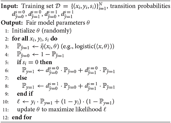
Algorithm 1. Fair learning with target labels ȳ
This section focuses on how to set values of the transition probabilities in order to arrive at balanced datasets.
Before we consider concrete values, we give some intuition for the transition probabilities. Let s = 0 refer to the protected group. For this group, we want to make more positive predictions than the training labels indicate. Variable ȳ is supposed to be our target proxy label. Thus, in order to make more positive predictions, some of the y = 0 labels should be associated with ȳ = 1. However, we do not know which. So, if our model predicts ȳ = 1 (high ℙ(ȳ = 1|x, θ)) while the training label is y = 0, then we allow for the possibility that this is actually correct. That is, ℙ(y = 0|ȳ = 1, s = 0) is not 0. If we choose, for example, ℙ(y = 0|ȳ = 1, s = 0) = 0.3 then that means that 30% of positive target labels ȳ = 1 may correspond to negative training labels y = 0. This way we can have more ȳ = 1 than y = 1, overall. On the other hand, predicting ȳ = 0 when y = 1 holds, will always be deemed incorrect: ℙ(y = 1|ȳ = 0, s = 0) = 0; this is because we do not want any additional negative labels.
For the non-protected group s = 1, we have the exact opposite situation. If anything, we have too many positive labels. So, if our model predicts ȳ = 0 (high ℙ(ȳ = 0|x, θ)) while the training label is y = 1, then we should again allow for the possibility that this is actually correct. That is, ℙ(y = 1|ȳ = 0, s = 1) should not be 0. On the other hand, ℙ(y = 0|ȳ = 1, s = 1) should be 0 because we do not want additional positive labels for s = 1. It could also be that the number of positive labels is exactly as it should be, in which case we can just set y = ȳ for all data points with s = 1.
A balanced dataset is characterized by an independence of the label ȳ and the sensitive attribute s. Given that we have complete control over the transition probabilities, we can ensure this independence by requiring ℙ(ȳ = 1|s = 0) = ℙ(ȳ = 1|s = 1). Our constraint is then that both of these probabilities are equal to the same value, which we will call the target rate PRt (“PR” as positive rate):
This leads us to the following constraints for s′ ∈ {0, 1}:
We call ℙ(y = 1|s = j) the base rate which we estimate from the training set:
Expanding the sum, we get
This is a system of linear equations consisting of two equations (one for each value of s′) and four free variables: ℙ(ȳ = 1|y, s) with y, s ∈ {0, 1}. The two unconstrained degrees of freedom determine how strongly the accuracy will be affected by the fairness constraint. If we set ℙ(ȳ = 1|y = 1, s) to 0.5, then this expresses the fact that a train label y of 1 only implies a target label ȳ of 1 in 50% of the cases. In order to minimize the effect on accuracy, we make ℙ(ȳ = 1|y = 1, s) as high as possible and ℙ(ȳ = 1|y = 0, s), conversely, as low as possible. However, the lowest and highest possible values are not always 0 and 1 respectively. To see this, we solve for ℙ(ȳ = 1|y = 0, s = j) in Equation (18):
If were greater than 1, then setting ℙ(ȳ = 1|y = 0, s = j) to 0 would imply a ℙ(ȳ = 1|y = 1, s = j) value greater than 1. A visualization that shows why this happens can be found in the Supplementary Material. We thus arrive at the following definitions:
Algorithm 2 shows pseudocode of the procedure, including the computation of the allowed minimal and maximal value.
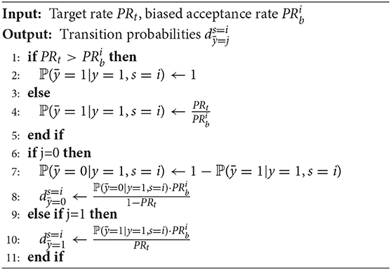
Algorithm 2. Targeting a balanced dataset
Once all these probabilities have been found, the transition probabilities needed for Equation (13) are fully determined by applying Bayes' rule:
As shown, there is a remaining degree of freedom when targeting a balanced dataset: the target rate PRt: = ℙ(ȳ = 1). This is true for both fairness criteria that we are targeting. The choice of targeting rate affects how much η and differ as implied by Theorem 1 (PRt affects ms and bs). should remain close to η as only represents an auxiliary distribution that does not have meaning on its own. The threshold ts in Theorem 1 (Equation 8) gives an indication of how close the distributions are. With the definitions in Equations (20) and (21), we can express ts in terms of the target rate and the base rate:
This shows that ts is smallest when and PRt are closest. However, as has different values for different s, we cannot set for all s. In order to keep both ts = 0 and ts = 1 small, it follows from Equation (23) that PRt should at least be between and . A more precise statement can be made when we explicitly want to minimize the sum ts = 0+ts = 1: assuming and , the optimal choice for PRt is (see Supplementary Material for details). We call this choice . For , analogous statements can be made, but this is of less interest as this case does not appear in our experiments.
The previous statements about ts do not directly translate into observable quantities like accuracy if the Tsybakov condition is not satisfied, and even if it is satisfied, the usefulness depends on the constants C and λ. Conversely, the following theorem makes generally applicable statement about the accuracy that can be achieved. Before we get to the theorem, we introduce some notation. We are given a dataset , where the xi are vectors of features and the yi the corresponding labels. We refer to the tuples (x, y) as the samples of the dataset. The number of samples is .
We assume binary labels (y ∈ {0, 1}) and thus can form the (disjoint) subsets and with
Furthermore, we associate each sample with a classification ŷ ∈ {0, 1}. The task of making the classification ŷ = 0 or ŷ = 1 can be understood as sorting each sample from into one of two sets: and , such that and .
We refer to the set as the set of correct (or accurate) predictions. The accuracy is given by .
Definition 2.
is called the base acceptance rate of the dataset .
Definition 3.
is called the predictive acceptance rate of the predictions.
Theorem 2. For a dataset with the base rate ra and corresponding predictions with a predictive acceptance rate of , the accuracy is limited by
Corollary 2.1. Given a dataset that consists of two subsets and () where p is the ratio of to and given corresponding acceptance rates and and predictions with target rates and , the accuracy is limited by
The proofs are fairly straightforward and can be found in the Supplementary Material.
Corollary 2.1 implies that in the common case where group s = 0 is disadvantaged () and also underrepresented (), the highest accuracy under demographic parity can be achieved at with
However, this means willingly accepting a lower accuracy in the (smaller) subset that is compensated by a very good accuracy in the (larger) subset . A decidedly “fairer” approach is to aim for the same accuracy in both subsets. This is achieved by using the average of the base acceptance rates for the target rate. As we balance the test set in our experiments, this kind of sacrificing of one demographic group does not work there. We compare the two choices ( and ) in section 5.
There is a fairness definition related to demographic parity which allows conditioning on “legitimate” risk factors ℓ when considering how equal the demographic groups are treated (Corbett-Davies et al., 2017). This cleanly translates into balanced datasets which are balanced conditioned on ℓ:
We can interpret this as splitting the data into partitions based on the value of ℓ, where the goal is to have all these partitions be balanced. This can easily be achieved by our method by setting a PRt(ℓ) for each value of ℓ and computing the transition probabilities for each sample depending on ℓ.
There are several ways to enforce fairness in machine learning models: as a pre-processing step (Kamiran and Calders, 2012; Zemel et al., 2013; Louizos et al., 2016; Lum and Johndrow, 2016; Chiappa, 2019; Quadrianto et al., 2019), as a post-processing step (Feldman et al., 2015; Hardt et al., 2016), or as a constraint during the learning phase (Calders et al., 2009; Zafar et al., 2017a,b; Donini et al., 2018; Dimitrakakis et al., 2019). Our method enforces fairness during the learning phase (an in-processing approach) but, unlike other approaches, we do not cast fair-learning as a constrained optimization problem. Constrained optimization requires a customized procedure. In Goh et al. (2016), Zafar et al. (2017a), and Zafar et al. (2017b), suitable majorization-minimization/convex-concave procedures (Lanckriet and Sriperumbudur, 2009) were derived. Furthermore, such constrained optimization approaches may lead to more unstable training, and often yield classifiers with both worse accuracy and more unfair (Cotter et al., 2018).
The approaches most closely related to ours were given by Kamiran and Calders (2012) who present four pre-processing methods: Suppression, Massaging the dataset, Reweighing, and Sampling. In our comparison we focus on methods 2, 3, and 4, because the first one simply removes sensitive attributes and those features that are highly correlated with them. All the methods given by Kamiran and Calders (2012) aim only at enforcing demographic parity.
The massaging approach uses a classifier to first rank all samples according to their probability of having a positive label (y = 1) and then flips the labels that are closest to the decision boundary such that the data then satisfies demographic parity. This pre-processing approach is similar in spirit to our in-processing method but differs in the execution. In our method (section 3.2), “ranking” and classification happen in one step and labels are not explicitly flipped but assigned probabilities of being flipped.
The reweighting method reweights samples based on whether they belong to an over-represented or under-represented demographic group. The sampling approach is based on the same idea but works by resampling instead of reweighting. Both reweighting and sampling aim to effectively construct a balanced dataset, without affecting the labels. This is in contrast to our method which treats the class labels as potentially untrustworthy and allows defying them.
One approach in Calders and Verwer (2010) is also worth mentioning. It is based on a generative Naïve Bayes model in which a latent variable L is introduced which is reminiscent to our target label ȳ. We provide a discriminative version of this approach. In discriminative models, parameters capture the conditional relationship of an output given an input, while in generative models, the joint distribution of input-output is parameterized. With this conditional relationship formulation (ℙ(y|ȳ, s) = ℙ(ȳ|y, s)ℙ(y|s)/ℙ(ȳ|s)), we can have detailed control in setting the target rate. Calders and Verwer (2010) focuses only on the demographic parity fairness metric.
We compare the performance of our target-label model with other existing models based on two real-world datasets. These datasets have been previously considered in the fairness-aware machine learning literature.
The proposed method is compatible with any likelihood-based algorithm. We consider both a non-parametric and a parametric model. The non-parametric model is a Gaussian process model, and logistic regression is the parametric counterpart. Since our fairness approach is not being framed as a constrained optimization problem, we can reuse off-the-shelf toolboxes including the GPyTorch library by Gardner et al. (2018) for Gaussian process models. This library incorporates recent advances in scalable variational inference including variational inducing inputs and likelihood ratio/REINFORCE estimators. The variational posterior can be derived from the likelihood and the prior. We need just need to modify the likelihood to take into account the target labels (Algorithm 1).
We run experiments on two real-world datasets. The first dataset is the Adult Income dataset (Dua and Graff, 2019). It contains 33,561 data points with census information from US citizens. The labels indicate whether the individual earns more (y = 1) or less (y = 0) than $50,000 per year. We use the dataset with either race or gender as the sensitive attribute. The input dimension, excluding the sensitive attributes, is 12 in the raw data; the categorical features are then one-hot encoded. For the experiments, we removed 2,399 instances with missing data and used only the training data, which we split randomly for each trial run. The second dataset is the ProPublica recidivism dataset. It contains data from 6,167 individuals that were arrested. The data was collected when investigating the COMPAS risk assessment tool (Angwin et al., 2016). The task is to predict whether the person was rearrested within two years (y = 1 if they were rearrested, y = 0 otherwise). We again use the dataset with either race or gender as the sensitive attributes.
Any fairness method that is targeting demographic parity, treats the training set as defective in one way: the acceptance rates are not equal in the training set and this needs to be corrected. As such, it does not make sense to evaluate these methods on a dataset that is equally defective. Predicting at equal acceptance rates is the correct result and the test set should reflect this.
In order to generate a test set which has the property of equal acceptance rates, we subsample the given, imbalanced, test set. For evaluating demographic parity, we discard datapoints from the imbalanced test set such that the resulting subset satisfies for all i and j. This balances the set in terms of s and ensures ℙ(y, s) = ℙ(y)ℙ(s), but does not force the acceptance rate to be , which in the case of the Adult dataset would be a severe change as the acceptance rate is naturally quite low there. Using the described method ensures that the minimal amount of data is discarded for the Adult dataset. We have empirically observed that all fairness algorithms benefit from this balancing of the test set.
The situation is different for equality of opportunity. A perfect classifier automatically satisfies equality of opportunity on any dataset. Thus, an algorithm aiming for this fairness constraint should not treat the dataset as defective. Consequently, for evaluating equality of opportunity we perform no balancing of the test set.
We evaluate two versions of our target label model1: FairGP, which is based on Gaussian Process models, and FairLR, which is based on logistic regression. We also train baseline models that do not take fairness into account.
In both FairGP and FairLR, our approach is implemented by modifying the likelihood function. First, the unmodified likelihood is computed (corresponding to ℙ(ȳ = 1|x, θ)) and then a linear transformation (dependent on s) is applied as given by Equation (13). No additional ranking of the samples is needed, because the unmodified likelihood already supplies ranking information.
The fair GP models and the baseline GP model are all based on variational inference and use the same settings. During training, each batch is equivalent to the whole dataset. The number of inducing inputs is 500 on the ProPublica dataset and 2500 on the Adult dataset which corresponds to approximately 1/8 of the number of training points for each dataset. We use a squared-exponential (SE) kernel with automatic relevance determination (ARD) and the probit function as the likelihood function. We optimize the hyper-parameters and the variational parameters using the Adam method (Kingma and Ba, 2015) with the default parameters. We use the full covariance matrix for the Gaussian variational distribution.
The logistic regression is trained with RAdam (Liu et al., 2019) and uses L2 regularization. For the regularization coefficient, we conducted a hyper-parameter search over 10 folds of the data. For each fold, we picked the hyper-parameter which achieved the best fairness among those 5 with the best accuracy scores. We then averaged over the 10 hyper-parameter values chosen in this way and then used this average for all runs to obtain our final results.
In addition to the GP and LR baselines, we compare our proposed model with the following methods: Support Vector Machine (SVM), Kamiran and Calders, 2012 (“reweighing” method), Agarwal et al., 2018 (using logistic regression as the classifier) and several methods given by Zafar et al. (2017a,b), which include maximizing accuracy under demographic parity fairness constraints (ZafarFairness), maximizing demographic parity fairness under accuracy constraints (ZafarAccuracy), and removing disparate mistreatment by constraining the false negative rate (ZafarEqOpp). Every method is evaluated over 10 repeats that each have different splits of the training and test set.
Following Zafar et al. (2017b), we evaluate demographic parity on the Adult dataset. Table 1 shows the accuracy and fairness for several algorithms. In the table, and in the following, we use PRs = i to denote the observed rate of positive predictions per demographic group ℙ(ŷ = 1|s = i). Thus, PRs = 0/PRs = 1 is a measure for demographic parity, where a completely fair model would attain a value of 1.0. This measure for demographic parity is also called “disparate impact” (see e.g., Feldman et al., 2015; Zafar et al., 2017a). As the results in Table 1 show, FairGP and FairLR are clearly fairer than the baseline GP and LR. We use the mean () for the target acceptance rate. The difference between fair models and unconstrained models is not as large with race as the sensitive attribute, as the unconstrained models are already quite fair there. The results of FairGP are characterized by high fairness and high accuracy. FairLR achieves similar results to FairGP, but with generally slightly lower accuracy but better fairness. We used the two step procedure of Donini et al. (2018) to verify that we cannot achieve the same fairness result with just parameter search on LR.
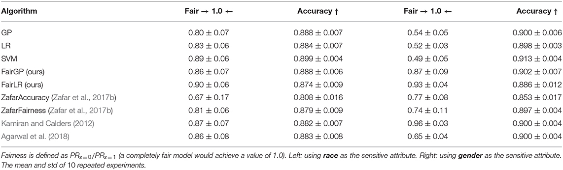
Table 1. Accuracy and fairness (with respect to demographic parity) for various methods on the balanced test set of the Adult dataset.
In Figure 1, we investigate which choice of target (, or ) gives the best result. We use for all following experiments as this is the fairest choice (cf. section 3.2). The Figure 1A shows results from Adult dataset with race as sensitive attribute where we have , and . performs best in term of the trade-off.
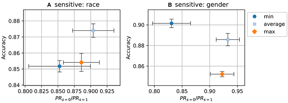
Figure 1. Accuracy and fairness (demographic parity) for various target choices. (A) Adult dataset using race as the sensitive attribute; (B) Adult dataset using gender. Center of the cross is the mean; height and width of the box encode half of standard derivation of accuracy and disparate impact.
Figures 2A,B show runs of FairLR where we explicitly set a target acceptance rate, PRt: = ℙ(ȳ = 1), instead of taking the mean . A perfect targeting mechanism would produce a diagonal. The plot shows that setting the target rate has the expected effect on the observed acceptance rate. This tuning of the target rate is the unique aspect of the approach. This would be very difficult to achieve with existing fairness methods; a new constraint would have to be added. The achieved positive rate is, however, usually a bit lower than the targeted rate (e.g., around 0.15 for the target 0.2). This is due to using imperfect classifiers; if TPR and TNR differ from 1, the overall positive rate is affected (see e.g., Forman, 2005 for discussion of this).
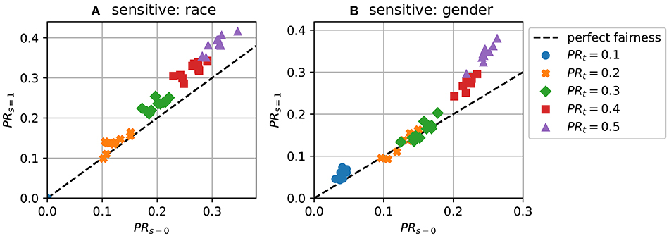
Figure 2. Predictions with different target acceptance rates (demographic parity) for 10 repeats. (A) PRs = 0 vs PRs = 1 using race as the sensitive attribute; (B) PRs = 0 vs PRs = 1 using gender.
Figures 3A,B show the same data as Figure 2 but with different axes. It can be seen from this Figures 3A,B that the fairness-accuracy trade-off is usually best when the target rate is close to the average of the positive rates in the dataset (which is around 0.2 for both sensitive attribute).
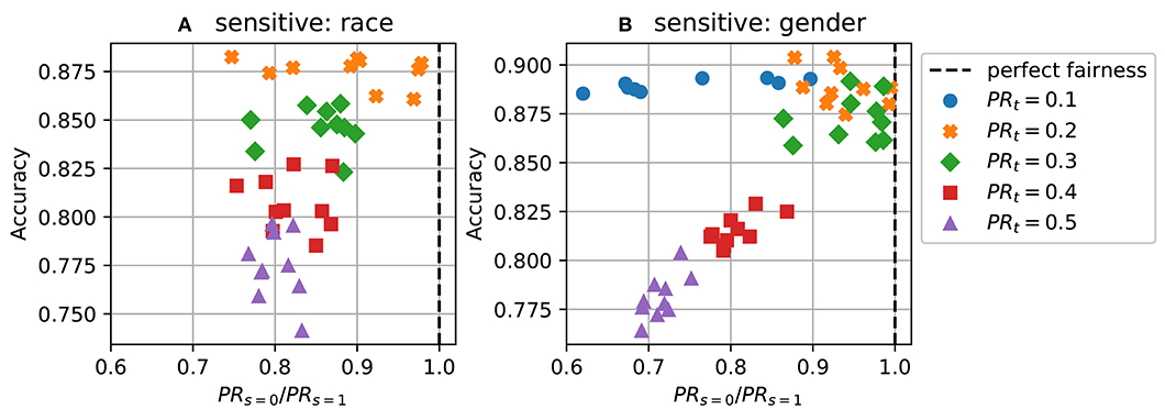
Figure 3. Predictions with different target acceptance rates (demographic parity) for 10 repeats. (A) Disparate impact vs accuracy on Adult dataset using race as the sensitive attribute; (B) Disparate impact vs accuracy using gender.
For equality of opportunity, we again follow Zafar et al. (2017a) and evaluate the algorithm on the ProPublica dataset. As we did for demographic parity, we define a measure of equality of opportunity via the ratio of the true positive rates (TPRs) within the demographic groups. We use TPRs = i to denote the observed TPR in group i: ℙ(ŷ = 1|y = 1, s = i), and TNRs = i for the observed true negative rate (TNR) in the same manner. The measure is then given by TPRs = 0/TPRs = 1. A perfectly fair algorithm would achieve 1.0 on the measure.
The results of 10 runs are shown in Figures 4, 5. Figures 4A,B show the accuracy-fairness trade-off; Figures 5A,B show the achieved TPRs. In the accuracy-fairness plot, varying PRt is shown to produce an inverted U-shape: Higher PRt still leads to improved fairness, but at a high cost in terms of accuracy.
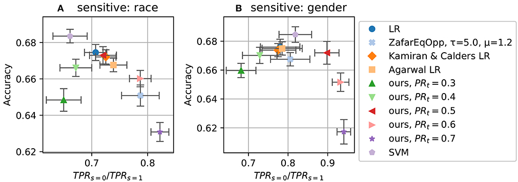
Figure 4. Accuracy and fairness (with respect to equality of opportunity) for various methods on ProPublica dataset. (A): using race as the sensitive attribute; (B): using gender. A completely fair model would achieve a value of 1.0 in the x-axis. See Figures 5A,B on how these choices of PR setting translate to TPRs = 0 vs TPRs = 1.
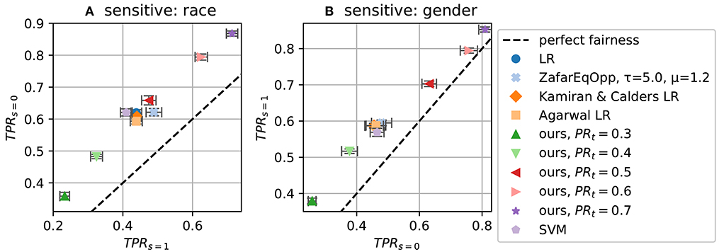
Figure 5. Fairness measure TPRs = 0 vs TPRs = 1 (equality of opportunity) for different target PRs (PRt). (A) On dataset ProPublica recidivism using race as the sensitive attribute; (B) using gender.
The latter two plots make clear that the TPR ratio does not tell the whole story: the realization of the fairness constraint can differ substantially. By setting different target PRs for our method, we can affect TPRs as well, where higher PRt leads to higher TPR, stemming from the fact that making more positive predictions increases the chance of making correct positive predictions.
Figure 5 shows that our method can span a wide range of possible TPR values. Tuning these hidden aspects of fairness is the strength of our method.
Fairness is fundamentally not a challenge of algorithms alone, but very much a sociological challenge. A lot of proposals have emerged recently for defining and obtaining fairness in machine learning-based decision making systems. The vast majority of academic work has focused on two categories of definitions: statistical (group) notions of fairness and individual notions of fairness (see Verma and Rubin, 2018 for at least twenty different notions of fairness). Statistical notions are easy to verify but do not provide protections to individuals. Individual notions do give individual protections but need strong assumptions, such as the availability of an agreed-upon similarity metric, which can be difficult in practice. We acknowledge that a proper solution to algorithmic fairness cannot rely on statistics alone. Nevertheless, these statistical fairness definitions can be helpful in understanding the problem and working toward solutions. To facilitate this, at every step, the trade-offs that are present should be made very clear and long-term effects have to be considered as well (Kallus and Zhou, 2018; Liu et al., 2018).
Here, we have developed a machine learning framework which allows us to learn from an implicit balanced dataset, thus satisfying the two most popular notions of fairness (Verma and Rubin, 2018), demographic parity (also known as avoiding disparate treatment) and equality of opportunity (or avoiding disparate mistreatment). Additionally, we indicate how to extend the framework to cover conditional demographic parity as well. The framework allows us to set a target rate to control how the fairness constraint is realized. For example, we can set the target positive rate for demographic parity to be 0.6 for different groups. Depending on the application, it can be important to specify whether non-discrimination ought to be achieved by more positive predictions or more negative predictions. This capability is unique to our approach and can be used as an intuitive mechanism to control the realization of fairness. Our framework is general and will be applicable for sensitive variables with binary and multi-level values. The current work focuses on a single binary sensitive variable. Future work could extend our tuning approach to other fairness concepts like the closely related predictive parity group fairness (Chouldechova, 2017) or individual fairness (Dwork et al., 2012).
The datasets generated for this study are available on request to the corresponding author.
All authors listed have made a substantial, direct and intellectual contribution to the work, and approved it for publication.
This work was supported by the UK EPSRC project EP/P03442X/1 EthicalML: Injecting Ethical and Legal Constraints into Machine Learning Models and the Russian Academic Excellence Project 5–100.
The authors declare that this study received funding from Nvidia Corporation and Amazon.com, Inc. The funder was not involved in the study design, collection, analysis, interpretation of data, the writing of this article or the decision to submit it for publication.
This manuscript has been released as a pre-print at arXiv (Kehrenberg et al., 2018). We gratefully acknowledge NVIDIA for GPU donations, and Amazon for AWS Cloud Credits. We thank Chao Chen and Songzhu Zheng for their inspiration of our main proof. The work by ZC was done while he was at the University of Sussex.
The Supplementary Material for this article can be found online at: https://www.frontiersin.org/articles/10.3389/frai.2020.00033/full#supplementary-material
1. ^The code can be found on GitHub: https://github.com/predictive-analytics-lab/ethicml-models/tree/master/implementations/fairgp.
Agarwal, A., Beygelzimer, A., Dudik, M., Langford, J., and Wallach, H. (2018). “A reductions approach to fair classification,” in ICML (Stockholm), Vol. 80, 60–69.
Angwin, J., Larson, J., Mattu, S., and Kirchner, L. (2016). Machine Bias. New York City, NY: ProPublica.
Barocas, S., and Selbst, A. D. (2016). Big data's disparate impact. California Law Rev. 104, 671–732. doi: 10.2139/ssrn.2477899
Bonilla, E. V., Krauth, K., and Dezfouli, A. (2016). Generic inference in latent Gaussian process models. arXiv preprint arXiv:1609.00577. Available online at: http://jmlr.org/papers/v20/16-437.html.
Calders, T., Kamiran, F., and Pechenizkiy, M. (2009). “Building classifiers with independency constraints,” in IEEE International Conference on Data mining Workshops, 2009. ICDMW'09 (Miami, FL: IEEE), 13–18. doi: 10.1109/ICDMW.2009.83
Calders, T., and Verwer, S. (2010). Three naive Bayes approaches for discrimination-free classification. Data Mining Knowledge Discov. 21, 277–292. doi: 10.1007/s10618-010-0190-x
Chiappa, S. (2019). “Path-specific counterfactual fairness,” in Proceedings of the AAAI Conference on Artificial Intelligence (Honolulu, HI), Vol. 33, 7801–7808. doi: 10.1609/aaai.v33i01.33017801
Chouldechova, A. (2017). Fair prediction with disparate impact: a study of bias in recidivism prediction instruments. Big Data 5, 153–163. doi: 10.1089/big.2016.0047
Corbett-Davies, S., Pierson, E., Feller, A., Goel, S., and Huq, A. (2017). “Algorithmic decision making and the cost of fairness,” in Proceedings of the 23rd ACM SIGKDD International Conference on Knowledge Discovery and Data Mining (Halifax), 797–806. doi: 10.1145/3097983.3098095
Cotter, A., Jiang, H., Wang, S., Narayan, T., Gupta, M. R., You, S., et al. (2018). Optimization with non-differentiable constraints with applications to fairness, recall, churn, and other goals. arXiv preprint arXiv:1809.04198. Available online at: http://jmlr.org/papers/v20/18-616
Creager, E., Madras, D., Jacobsen, J.-H., Weis, M., Swersky, K., Pitassi, T., et al. (2019). “Flexibly fair representation learning by disentanglement,” in International Conference on Machine Learning (ICML), Volume 97 of Proceedings of Machine Learning Research, eds K. Chaudhuri and R. Salakhutdinov (Long Beach, CA: PMLR), 1436–1445.
Dimitrakakis, C., Liu, Y., Parkes, D. C., and Radanovic, G. (2019). “Bayesian fairness,” in Proceedings of the AAAI Conference on Artificial Intelligence (Honolulu, HI), Vol. 33, 509–516. doi: 10.1609/aaai.v33i01.3301509
Donini, M., Oneto, L., Ben-David, S., Shawe-Taylor, J. S., and Pontil, M. (2018). “Empirical risk minimization under fairness constraints,” in NeurIPS (Montreal), 2796–2806.
Dua, D., and Graff, C. (2019). UCI Machine Learning Repository. Irvine, CA: University of California, School of Information and Computer Science. Available online at: https://archive.ics.uci.edu/ml/citation_policy.html
Dwork, C., Hardt, M., Pitassi, T., Reingold, O., and Zemel, R. (2012). “Fairness through awareness,” in Proceedings of the 3rd Innovations in Theoretical Computer Science Conference (Cambridge, MA: ACM), 214–226. doi: 10.1145/2090236.2090255
Feldman, M., Friedler, S. A., Moeller, J., Scheidegger, C., and Venkatasubramanian, S. (2015). “Certifying and removing disparate impact,” in Proceedings of the 21th ACM SIGKDD International Conference on Knowledge Discovery and Data Mining (Sydney: ACM), 259–268. doi: 10.1145/2783258.2783311
Forman, G. (2005). “Counting positives accurately despite inaccurate classification,” in European Conference on Machine Learning (Springer), 564–575. doi: 10.1007/11564096_55
Gardner, J. R., Pleiss, G., Bindel, D., Weinberger, K. Q., and Wilson, A. G. (2018). “GPyTorch: blackbox matrix-matrix gaussian process inference with GPU acceleration,” in NeurIPS (Montreal), 7587–7597.
Goh, G., Cotter, A., Gupta, M., and Friedlander, M. P. (2016). “Satisfying real-world goals with dataset constraints,” in Advances in Neural Information Processing Systems (NIPS), eds D. D. Lee, M. Sugiyama, U. V. Luxburg, I. Guyon, and R. Garnett, 2415–2423.
Hardt, M., Price, E., and Srebro, N. (2016). “Equality of opportunity in supervised learning,” in Advances in Neural Information Processing Systems, eds D. D. Lee, M. Sugiyama, U. V. Luxburg, I. Guyon, and R. Garnett (Barcelona: Curran Associates, Inc.), 3315–3323.
Joseph, M., Kearns, M., Morgenstern, J. H., and Roth, A. (2016). “Fairness in learning: classic and contextual bandits,” in NIPS (Barcelona), 325–333.
Kallus, N., and Zhou, A. (2018). “Residual unfairness in fair machine learning from prejudiced data,” in Proceedings of the 35th International Conference on Machine Learning (Stockholm), Vol. 80, 2439–2448.
Kamiran, F., and Calders, T. (2012). Data preprocessing techniques for classification without discrimination. Knowledge Inform. Syst. 33, 1–33. doi: 10.1007/s10115-011-0463-8
Kamishima, T., Akaho, S., Asoh, H., and Sakuma, J. (2012). “Fairness-aware classifier with prejudice remover regularizer,” in Joint European Conference on Machine Learning and Knowledge Discovery in Databases (Bristol: Springer), 35–50. doi: 10.1007/978-3-642-33486-3_3
Kehrenberg, T., Chen, Z., and Quadrianto, N. (2018). Tuning fairness by marginalizing latent 1target labels. arXiv preprint arXiv:1810.05598.
Kingma, D. P., and Ba, J. (2015). “Adam: a method for stochastic optimization,” in 3rd International Conference on Learning Representations, ICLR 2015, eds Y. Bengio and Y. LeCun (San Diego).
Krauth, K., Bonilla, E. V., Cutajar, K., and Filippone, M. (2016). AutoGP: Exploring the capabilities and limitations of Gaussian Process models. arXiv preprint arXiv:1610.05392.
Lanckriet, G. R., and Sriperumbudur, B. K. (2009). “On the convergence of the concave-convex procedure,” in Advances in Neural Information Processing Systems (NIPS), eds Y. Bengio, D. Schuurmans, J. D. Lafferty, C. K. I. Williams, and A. Culotta (Vancouver, BC: Curran Associates, Inc.), 1759–1767.
Liu, L., Jiang, H., He, P., Chen, W., Liu, X., Gao, J., et al. (2019). On the variance of the adaptive learning rate and beyond. arXiv preprint arXiv:1908.03265.
Liu, L. T., Dean, S., Rolf, E., Simchowitz, M., and Hardt, M. (2018). “Delayed impact of fair machine learning,” in Proceedings of the 35th International Conference on Machine Learning (Stockholm), Vol. 80, 3150–3158. doi: 10.24963/ijcai.2019/862
Louizos, C., Swersky, K., Li, Y., Welling, M., and Zemel, R. (2016). “The variational 1fair autoencoder,” in International Conference on Learning Representations (ICLR) (San Juan).
Lum, K., and Johndrow, J. (2016). A statistical framework for fair predictive algorithms. arXiv preprint arXiv:1610.08077.
Olteanu, A., Castillo, C., Diaz, F., and Kiciman, E. (2019). Social data: biases, methodological pitfalls, and ethical boundaries. Front. Big Data 2:13. doi: 10.3389/fdata.2019.00013
Quadrianto, N., and Sharmanska, V. (2017). “Recycling privileged learning and distribution matching for fairness,” in Advances in Neural Information Processing Systems (Long Beach, CA), 677–688.
Quadrianto, N., Sharmanska, V., and Thomas, O. (2019). “Discovering fair representations in the data domain,” in Computer Vision and Pattern Recognition (CVPR) (Long Beach, CA: Computer Vision Foundation/IEEE), 8227–8236. doi: 10.1109/CVPR.2019.00842
Tolan, S. (2019). Fair and unbiased algorithmic decision making: Current state and future challenges. arXiv preprint arXiv:1901.04730.
Tsybakov, A. B. (2004). Optimal aggregation of classifiers in statistical learning. Ann. Stat. 32, 135–166. doi: 10.1214/aos/1079120131
Verma, S., and Rubin, J. (2018). “Fairness definitions explained,” in 2018 IEEE/ACM International Workshop on Software Fairness (FairWare) (Gothenburg: IEEE), 1–7. doi: 10.1145/3194770.3194776
Zafar, M. B., Valera, I., Gomez Rodriguez, M., and Gummadi, K. P. (2017a). “Fairness beyond disparate treatment & disparate impact: Learning classification without disparate mistreatment,” in Proceedings of the 26th International Conference on World Wide Web (Perth: International World Wide Web Conferences Steering Committee), 1171–1180. doi: 10.1145/3038912.3052660
Zafar, M. B., Valera, I., Rogriguez, M. G., and Gummadi, K. P. (2017b). “Fairness constraints: mechanisms for fair classification,” in Artificial Intelligence and Statistics (Fort Lauderdale), 962–970.
Keywords: algorithmic bias, fairness, machine learning, demographic parity, equality of opportunity
Citation: Kehrenberg T, Chen Z and Quadrianto N (2020) Tuning Fairness by Balancing Target Labels. Front. Artif. Intell. 3:33. doi: 10.3389/frai.2020.00033
Received: 18 February 2020; Accepted: 15 April 2020;
Published: 12 May 2020.
Edited by:
Fabrizio Riguzzi, University of Ferrara, ItalyCopyright © 2020 Kehrenberg, Chen and Quadrianto. This is an open-access article distributed under the terms of the Creative Commons Attribution License (CC BY). The use, distribution or reproduction in other forums is permitted, provided the original author(s) and the copyright owner(s) are credited and that the original publication in this journal is cited, in accordance with accepted academic practice. No use, distribution or reproduction is permitted which does not comply with these terms.
*Correspondence: Thomas Kehrenberg, dC5rZWhyZW5iZXJnQHN1c3NleC5hYy51aw==
†Present address: Zexun Chen, BioComplex Laboratory, Computer Science, University of Exeter, Exeter, United Kingdom
Disclaimer: All claims expressed in this article are solely those of the authors and do not necessarily represent those of their affiliated organizations, or those of the publisher, the editors and the reviewers. Any product that may be evaluated in this article or claim that may be made by its manufacturer is not guaranteed or endorsed by the publisher.
Research integrity at Frontiers
Learn more about the work of our research integrity team to safeguard the quality of each article we publish.