
95% of researchers rate our articles as excellent or good
Learn more about the work of our research integrity team to safeguard the quality of each article we publish.
Find out more
ORIGINAL RESEARCH article
Front. Aquac. , 09 July 2024
Sec. Disease and Health Management
Volume 3 - 2024 | https://doi.org/10.3389/faquc.2024.1365123
This article is part of the Research Topic Aquatic Animal Health and Epidemiology: Disease Surveillance, Prevention and Control View all 7 articles
 Vitor Cerqueira1*
 João Pimentel1,2
 Jennie Korus3
 Francisco Bravo4
 Joana Amorim1,2
 Mariana Oliveira1Andrew Swanson5
 Ramón Filgueira6
 Jon Grant7
 Luis Torgo1
Introduction: Hypoxia is defined as a critically low-oxygen condition of water, which, if prolonged, can be harmful to fish and many other aquatic species. In the context of ocean salmon fish farming, early detection of hypoxia events is critical for farm managers to mitigate these events to reduce fish stress, however in complex natural systems accurate forecasting tools are limited. The goal of this research is to use a machine learning approach to forecast oxygen concentration and predict hypoxia events in marine net-pen salmon farms.
Methods: The developed model is based on gradient boosting and works in two stages. First, we apply auto-regression to build a forecasting model that predicts oxygen concentration levels within a cage. We take a global forecasting approach by building a model using the historical data provided by sensors at several marine fish farms located in eastern Canada. Then, the forecasts are transformed into binary probabilities that indicate the likelihood of a low-oxygen event. We leverage the cumulative distribution function to compute these probabilities.
Results and discussion: We tested our model in a case study that included several cages across 14 fish farms. The experiments suggest that the model can detect future hypoxic events with a commercially acceptable false alarm rate. The resulting probabilistic predictions and oxygen concentration forecasts can help salmon farmers to prioritize resources, and reduce harm to crops.
Fish farms produce large quantities of marine protein efficiently, reducing pressure on wild fish populations. They promote biodiversity and thus, the sustainability of wild fishing operations (Subasinghe et al., 2009). Overall, fish farms are an increasingly important food production system in our society for both economic and environmental reasons, e.g. reducing overfishing.
Good farm management and fish health, critically require reduction of fish stress and the ability to detect poor water quality. In this regard, one of the main challenges for ocean farms is maintaining optimal levels of dissolved oxygen in cages. Variable farm conditions such as high water temperatures, algae blooms, and or high stocking densities can all exasperate oxygen availability, potentially triggering a low-oxygen event (Yokoyama, 1997; Burke et al., 2021). These events, also referred to as hypoxia episodes, occur when the oxygen level in the water falls below 7mgL−1 (Oppedal et al., 2011), though the severity depends on the specific farm environment, age of salmon, and the available reactive mitigation tools (i.e., oxygen dispersal systems) (Remen, 2012).
Hypoxia events cause stress to fish, negatively impacting fish welfare and productivity, and in the most severe cases can lead to mortalities, causing significant economic loss to producers. As such, the availability of more accurate hypoxia prediction tools would both improve the well-being of fish and the economic management of farms. Similarly, this tool could help farmers reduce significant costs associated with mitigation technologies.
The goal of this work is to build a model to i) forecast oxygen concentration and ii) predict hypoxia events on farms using machine learning. Specifically, at each time step, we aim to predict the probability that the oxygen level will fall below a critical threshold. A probabilistic approach is useful to decision-makers within farms. For example, if there is a high likelihood of a low-oxygen event, a farmer can proactively turn on mitigation systems rather than waiting for the low-oxygen event to occur, which can cause stress to fish, and delay return to more optimal oxygen levels.
The probabilistic forecasting of binary events is usually tackled as a classification problem. However, a classifier is unable to predict the future values of oxygen – only the likelihood of a hypoxic event. Complementing event probability estimates with oxygen forecasts is valuable for having both an efficient means to alert operators of impending low dissolved oxygen events and the ability to analyze temporal trends in dissolved oxygen. In effect, we apply an auto-regressive approach to forecast oxygen dynamics. Then, we resort to the cumulative distribution function to convert these forecasts into a hypoxic event probability following Cerqueira and Torgo (2022).
The developed model was validated using data from 14 fish farms located in different locations across eastern Canada. Each farm contains several cages where fish are grown in variable stocking densities, leading to different micro-climates for each cage. The results of the experiments showed that the model was able to accurately predict critical events at the cage level on each of the farms. Overall, this case study demonstrated the effectiveness of using machine learning to forecast critical events in ocean fish farms.
In this section, we present the case study used in this work. We start by describing the data structure and its main characteristics (Section 2.1). We also carry out an exploratory data analysis to uncover valuable insights before building a forecasting model (Section 2.2).
We can define a database of fish farms as . Each fish farm contains several cages , where mF is the number of cages in the farm. Finally, each cage can be represented as a time series , where is the observation of cage at time i and is the number of observations in the cage. Each observation contains information about the oxygen concentration in the cage (in ). Effectively, each cage consists of a univariate time series. In the original dataset, other information was available, such as temperature or cage depth. However, in the experiments, variables other than oxygen concentration were not found to improve the hypoxia detection accuracy of the model. Therefore, these were excluded from the model.
The case study comprises data collected from 14 fish farms located in different places across eastern Canada. The data ranges over five years, from 2017 to 2023. The sampling period is detailed in Table 1. The observations of each time series are captured with a high but, due to operator stocking plans, irregular sampling frequency. The period between consecutive observations can range from 1 to 3 minutes. We aim to forecast hourly values of oxygen concentration. Therefore, we aggregated the data in each cage to an hourly granularity. This is accomplished by taking the median of the collected values of each hour. If no observation was captured in a given hour this represented a missing observation. As an example, Figure 1 illustrates a sample of the time series of oxygen concentration in a given cage.
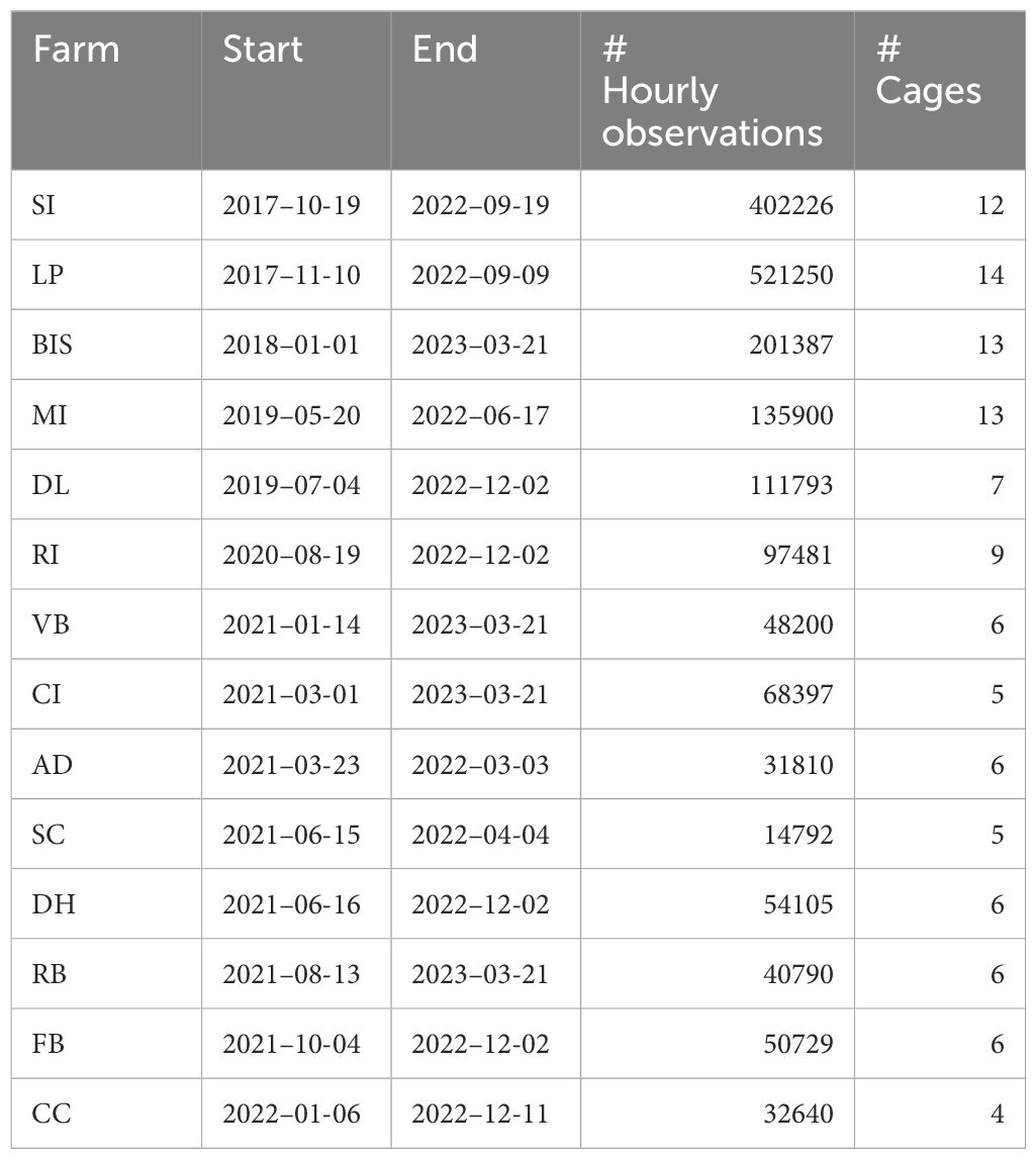
Table 1 General information about the fish farms in the case study.
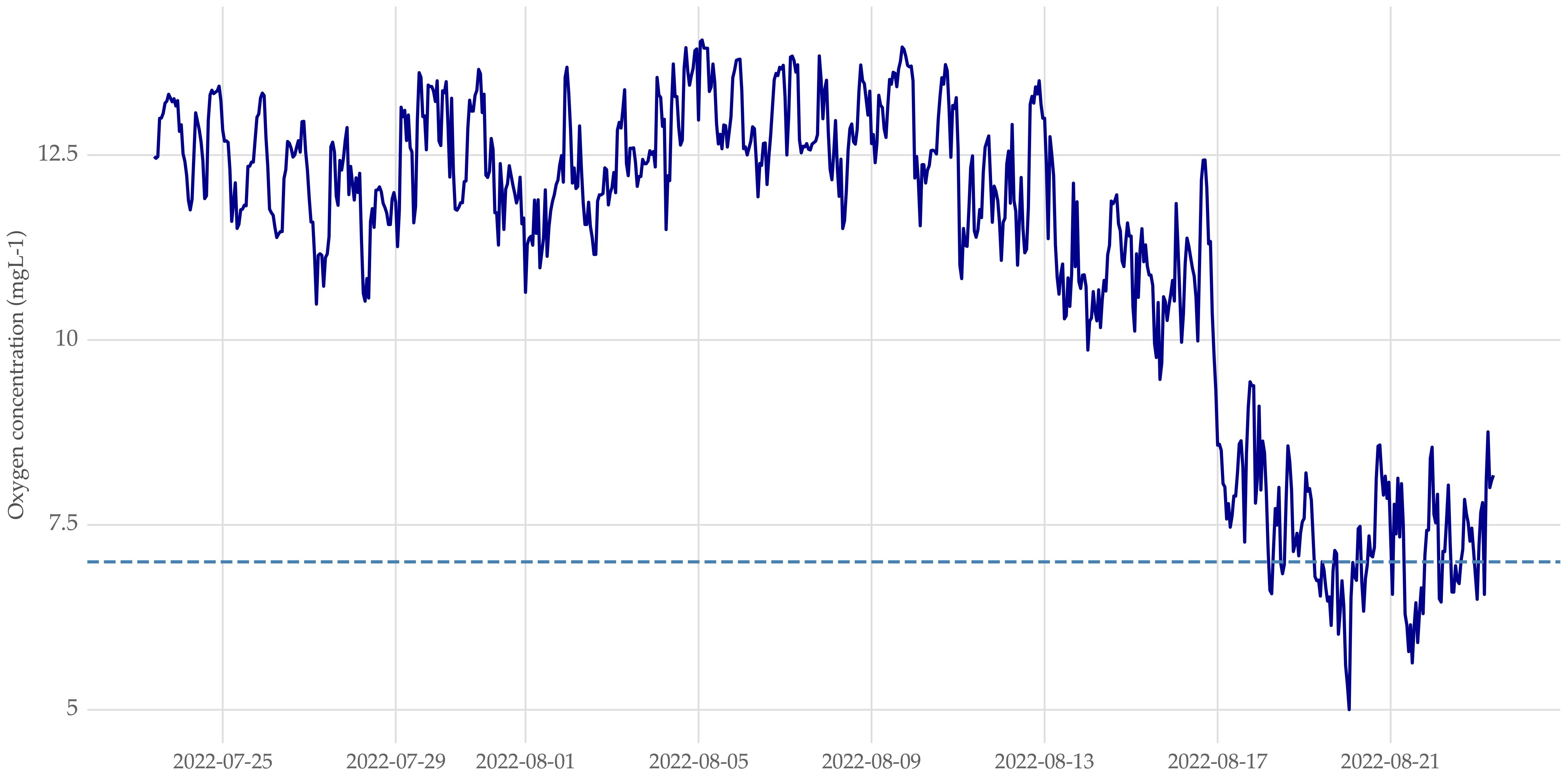
Figure 1 Sample of the oxygen concentration time series in a cage within the LP fish farm. The horizontal dashed line denotes the threshold below which hypoxia occurs (7 mgL−1).
Figure 2 shows the number of data points over each month by fish farm, from October 2017 to December 2022. Until 2019, the data came from only two farms (SI and LP). The data for the year 2022 comprises the most data points, while there is a period with very little data during 2018.
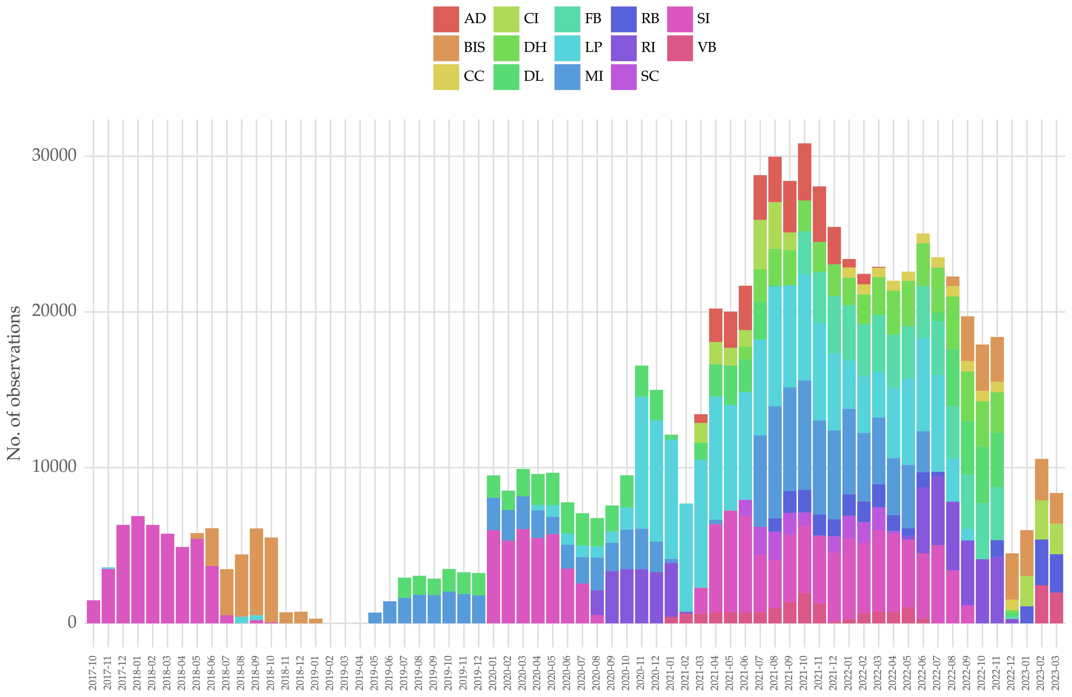
Figure 2 Number of data points by month and fish farm.
We carried out an extensive exploratory data analysis to draw insights about the oxygen concentration dynamics. We illustrate the main findings in this section. Figure 3 shows the oxygen concentration over time at each farm. For visualization purposes, we aggregated the data in each farm by taking the median across all available cages. Overall, this plot indicates the presence of yearly seasonality influencing oxygen concentration.
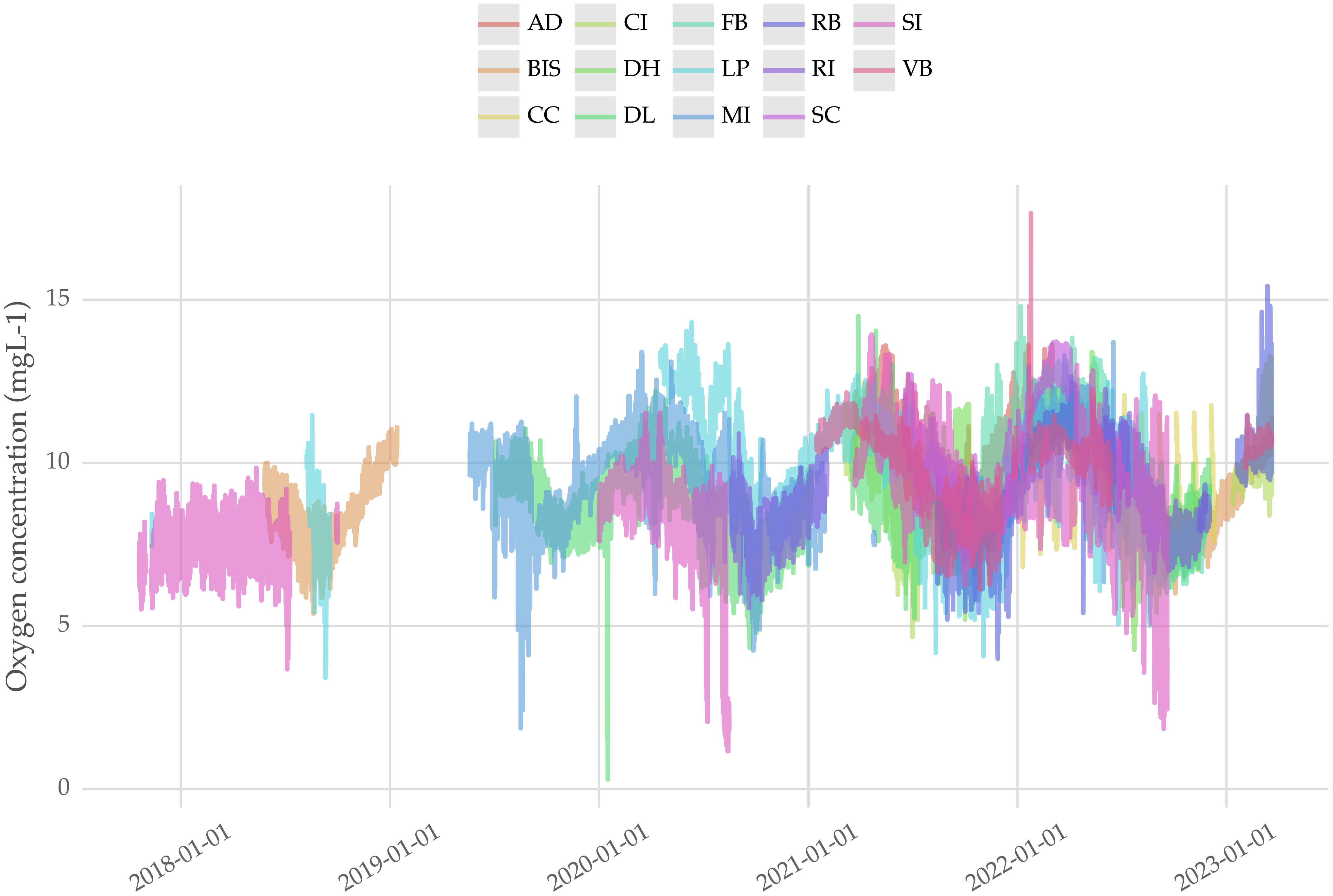
Figure 3 Hourly oxygen concentration time series by farm. The values of the time series are aggregated (median) by cage. The plot suggests similar dynamics across farms and yearly seasonality.
There are some periods of missing data, especially in the years 2018 and 2019. The mechanisms behind the missingness are either missing completely at random (e.g. random sensor malfunction in a given observation) or missing at random (e.g. sensor shutdown during some period for maintenance), according to the definitions described by Schafer and Graham (2002).
We explored the distribution of oxygen concentration using violin plots in Figure 4. For this analysis, we studied each farm as a whole and disregarded information about individual cages. Overall, the distribution varies across farms. Besides the different locations of each farm, one possible reason for this variability was the sampling period at each farm is different, covering various lengths of time and capturing data during different seasons which is known to influence oxygen fluctuations (Burke et al., 2021).

Figure 4 Distribution of oxygen concentration (mgL−1) by farm.
This work is devoted to the prediction of hypoxia events, which can be defined as an observation with an oxygen concentration below 7 mgL−1 (Oppedal et al., 2011). In this context, we analyzed the distribution of the oxygen condition (normal or hypoxia) across fish farms and over different months. Figure 5 shows the relative frequency (%) of each condition across all observations at each fish farm. Hypoxia is generally a rare occurrence across all farms; however, events are more common at some farms such as DH and SI compared to others. Figure 6 also shows that hypoxia is more common during the summer and fall seasons. This is expected as these events are correlated with higher water temperatures, which reduces the solubility of oxygen in seawater (Burke et al., 2021).
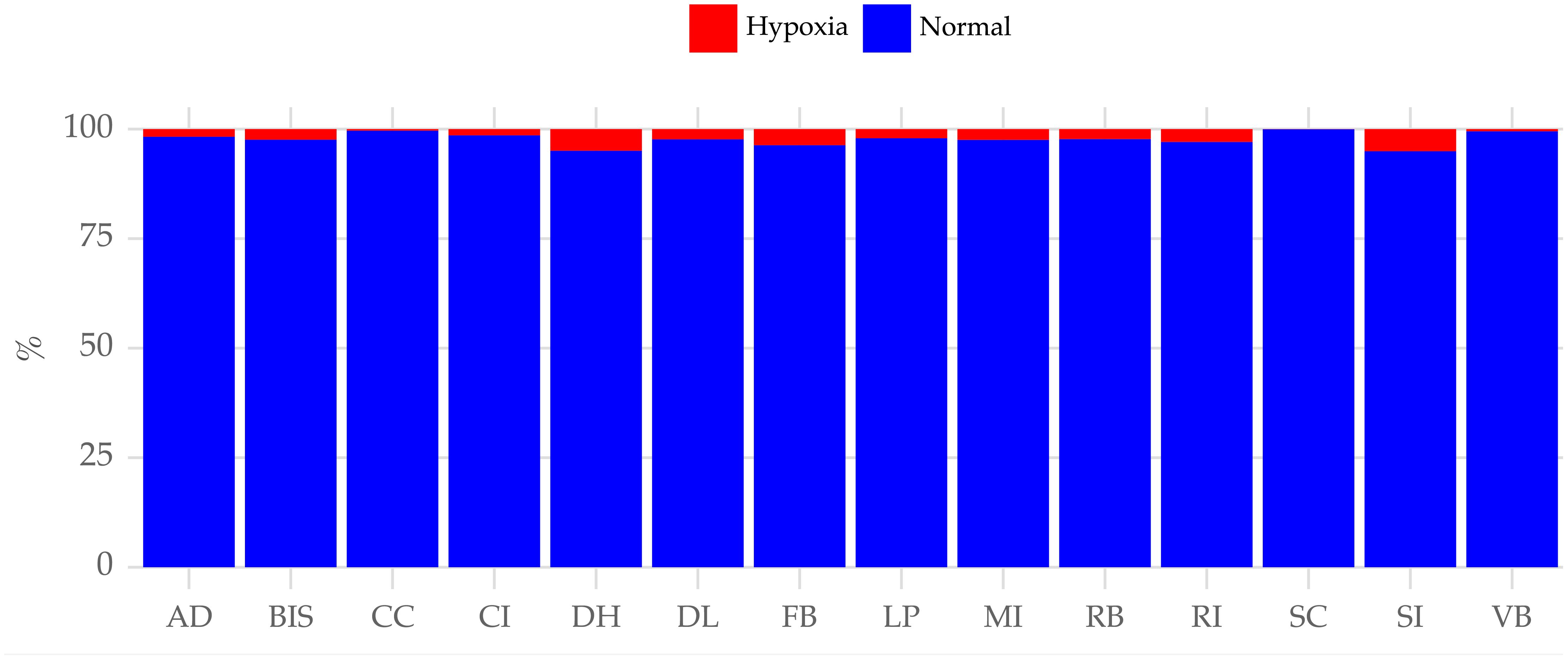
Figure 5 Distribution of oxygen concentration condition across fish farms. Hypoxia (< 7mgL−1) conditions are more common in some farms than others.
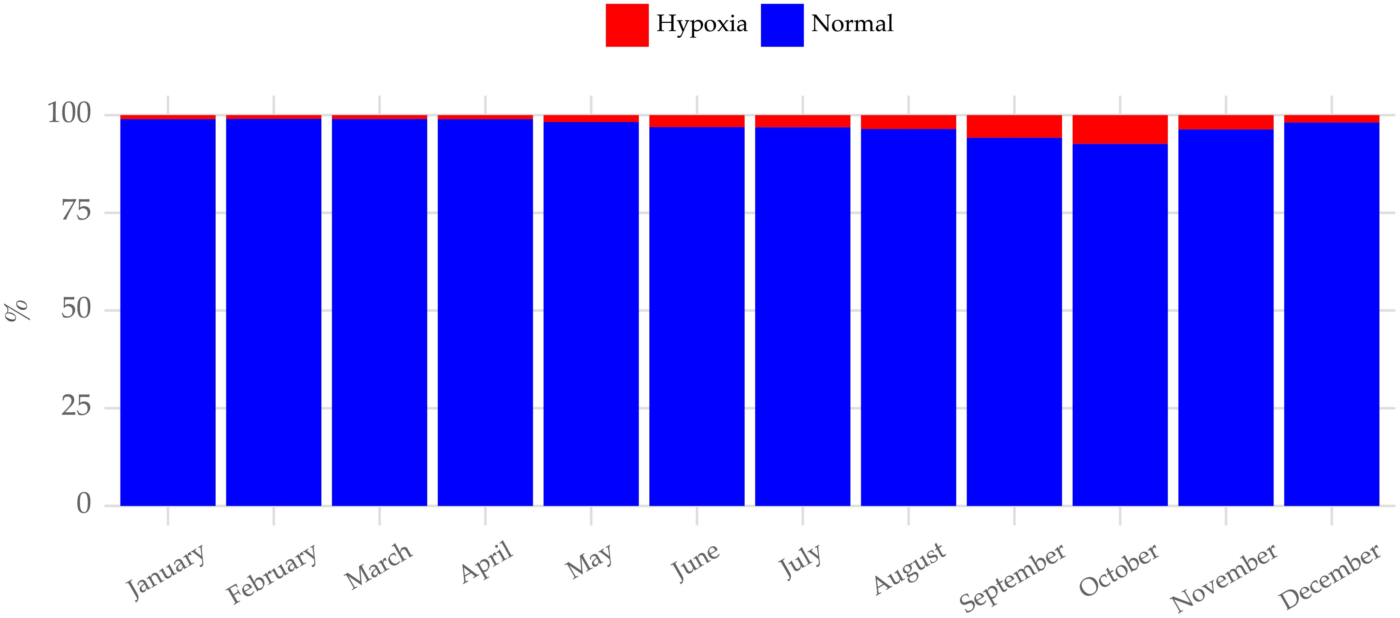
Figure 6 Distribution of oxygen concentration condition across each month. Hypoxic (< 7mgL-1) conditions are more common in the summer and fall seasons.
This section describes the background of this work. We start by formalizing the forecasting task as an auto-regressive problem (Section 3.1). Then, we explain how this formalization extends to the exceedance probability estimation setting (Section 3.3). We also describe how global forecasting models operate and how they relate to our work (Section 3.2). Finally, in Section 3.4, we carry out a brief literature review and describe previous efforts in forecasting oxygen dynamics. We remark that the background provided here focuses on statistical and machine learning models, and does not consider deterministic biogeochemical models that also have been used to predict oxygen at salmon farm sites (e.g (Wild-Allen et al., 2020)).
The general goal behind forecasting is to predict the value of the upcoming observations of oxygen concentration in a given cage, , given the historical data, where h denotes the forecasting horizon.
We formalize the problem of time series forecasting based on an auto-regressive strategy. Accordingly, observations of a time series are modeled based on their recent lags. More precisely, the value of ci is modeled based on the most recent timesteps: , where is the observation we want to predict and represents the corresponding input lagged features (Bontempi et al., 2013). This approach leads to a multiple regression problem where the temporal dependency is modeled by using past observations as explanatory variables. Using h = 1 for illustration purposes, the goal is to transform each time series into a matrix structure as follows:
Each row in the matrix above is a sample (X,c). The last column of the matrix denotes the target variable (future observations) and the remaining columns represent the lagged explanatory variables (X). denotes the reconstructed time series in a matrix structure for a given cage . For each forecasting horizon , the goal is to build a multiple regression model that can be written as , where represents additional covariates known at the i-th instance. These covariates can be, for example, explanatory time series related to the phenomenon. For example, the season of the year.
Traditionally, forecasting models are trained using the historical data of the time series of interest, often referred to as local models (Januschowski et al., 2020). In our case, we need to forecast time series from several cages that belong to multiple fish farms. Leveraging the historical observations of all available time series can be valuable to build a forecasting model. The dynamics of the time series are often related, and a model may be able to learn useful patterns from some time series that have not revealed themselves in others. Models that are trained on multiple time series are often referred to as global forecasting models (Godahewa et al., 2021).
The popularity of global forecasting methods has surged following their successful use in the M4 forecasting competition, which featured 100000 time series from different application domains. The contest was won by a global forecasting method developed by Smyl (2020) that combines an exponential smoothing method with a recurrent neural network. Since then, several other works have been developed for training forecasting models with multiple time series (Godahewa et al., 2021).
The key motivation for our use of a global forecasting approach is giving the learning algorithm access to additional data. Machine learning algorithms tend to perform better with larger training sets, especially those with many parameters (Cerqueira et al., 2022). We will build a global model to forecast oxygen concentration based on the available information across all cages from all fish farms.
Conveying the uncertainty around forecasts is critical for better decision-making. Uncertainty in numerical forecasts is usually quantified by predicting intervals (Khosravi et al., 2011), or probabilities (Gneiting and Katzfuss, 2014).
For binary events, we can simply output the probability of that event occurring. An instance of a binary event is exceedance, which, as mentioned before, refers to when a time series exceeds a predefined threshold.
The probability of a hypoxia event hi denotes the probability that the oxygen concentration ci falls below 7 mgL−1 in any given instant i. In this type of problem, hi is usually modeled by resorting to a binary target variable bi, which can be formalized as shown in Equation 1:
This setting leads to a classification problem where the goal is to build a classifier g of the form bi = g(Xi). Logistic regression is commonly used for this purpose (Taylor and Yu, 2016). However, in our problem, a classification model would be unable to output the numeric oxygen forecasts which can be important for on-farm decision-making. Accordingly, in Section 4, we present an alternative approach to standard classification.
Understanding and forecasting water quality and oxygen dynamics is a relevant task and many works have been devoted to it (Zhang et al., 2022; Hai et al., 2023; Zhao et al., 2023). Liu et al. (2021) developed an ensemble based on Bayesian model averaging using a hybrid approach that includes artificial neural networks. Therein, the authors outline several state-of-the-art approaches to forecasting dissolved oxygen in the context of aquaculture.
Several works address the problem of detecting hypoxic events using data-driven methods. Arepalli and Naik (2024) tackle this problem using a deep learning method based on self-attention and LSTM layers. Besides dissolved oxygen, they also use other input variables such as temperature or turbidity. They report 99.8% accuracy, though this metric is usually a poor choice for problems involving imbalanced distributions (Bronco et al., 2016). Similar to us, Politicos et al. (2021) modeled hypoxia using tree-based models and reported an F1 score ranging between 0.84 and 0.93. The F1 score is a classification metric that combines precision and recall measures. However, while we deal with North Atlantic ocean data, the data used in their study was collected from an enclosed lagoon in the Greek Mediterranean.
We aim to predict hypoxic events and forecast oxygen concentration using a single model, whereas previous research addresses only one of these problems. As mentioned before, coupling forecasts with hypoxia probabilities can be useful to foster more informed decision-making by farmers.
In this section, we describe the proposed approach for estimating the probability of hypoxia events in fish farms. We start by describing the forecasting approach based on a global model and how it is used to compute probabilistic estimates (Section 4.1). Then, we explain how the proposed method is evaluated (Section 4.2).
The development of the model works in three main steps:
1. Data preparation;
2. Building a forecasting model based on a global strategy;
3. Convert the forecasts produced by the model into probability estimates of hypoxia.
In the next subsections, we explain each step in turn.
Several data preparation steps were carried out before training a model. The workflow is summarized in Figure 7. During the data preparation stage, we conducted a time series analysis using hypothesis testing to assess the presence of trend, seasonality, and heteroscedasticity in the data concerning each cage.
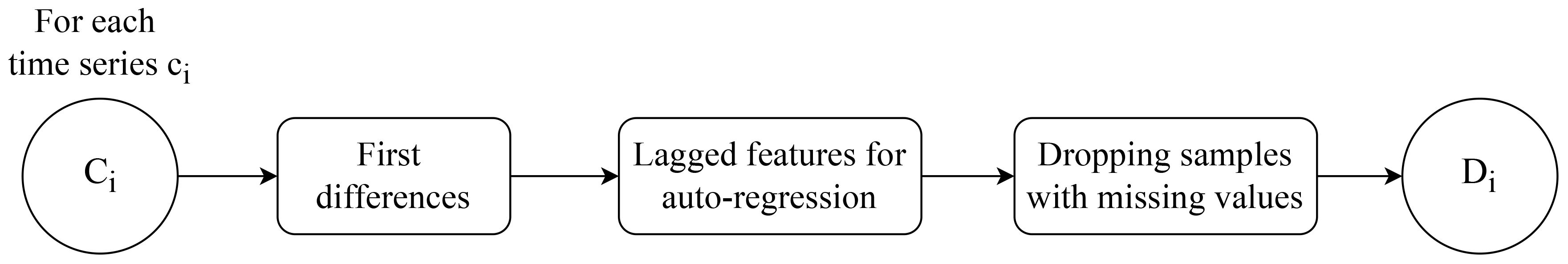
Figure 7 Data preparation workflow.
Regarding trend, we used the KPSS test (Kwiatkowski et al., 1992) to assess if differencing was required for stationarity. We conducted yearly seasonal differencing before applying the hypothesis test to control for seasonal effects. The column Trend in Table 2 reports the ratio of cages in a given fish farm where the null hypothesis that the time series is trend-stationary is rejected with a significance value of 0.05. The null hypothesis is not rejected in all cases. However, in the interest of consistency and to keep all observations in a common value range, we took first differences in all-time series.
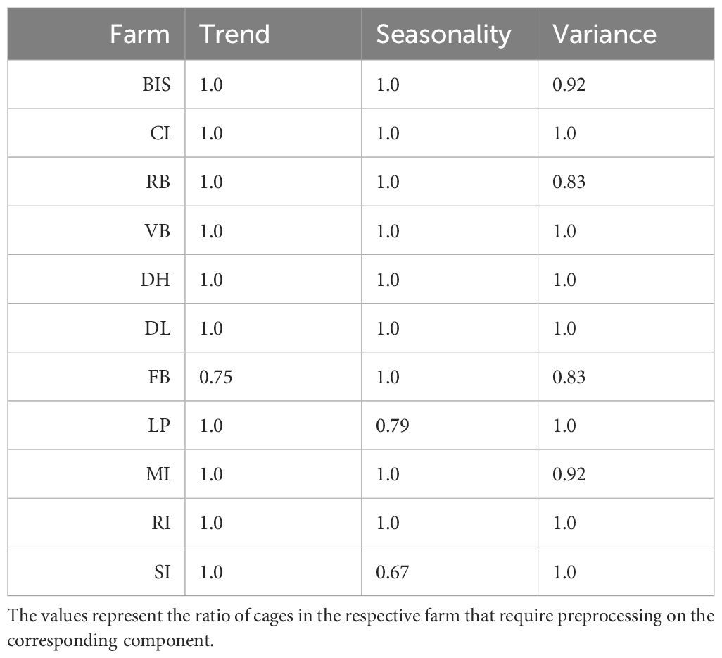
Table 2 Results of time series analysis for each fish farm.
Visual inspection (c.f. Figure 1) indicated the presence of a strong yearly seasonal effect. We applied the heuristic by Wang et al. (2006) to measure the seasonal strength. They consider the presence of a relevant seasonal component if the seasonal strength is above 0.641. The column Seasonality in Table 2 reports the ratio of times that this occurs across each fish farm. The results corroborated the visual inspection. In effect, we attempted to account for seasonal variations using either Fourier series with yearly periods and monthly dummy variables. However, none of these approaches improved forecasting performance and were thus excluded from the model. We hypothesize that the first differences preprocessing operation has a sufficient stabilization effect and that it smooths out seasonal variations. Seasonality was checked in daily and weekly periodicity but the results did not give evidence for the presence of this component (results not showed).
Finally, we also checked whether each time series is heteroskedastic using the White test (White, 1980). The column Variance in Table 2 shows the ratio of cages in which the null hypothesis of equal variance was rejected with a significance value below 0.05. The results suggest that the time series are heteroskedastic, and we attempted to stabilize the variance of the data by taking the logarithm. This transformation did not improve forecasting accuracy, so it was also excluded from the final model.1
After this analysis, we transformed each time series for supervised learning using the process outlined in Section 3.1. This involves computing lagged features for an auto-regressive modeling approach, with a forecasting horizon h from 1 to 24. The number of lags p is set to 24. This means that, at each time step, a model produces forecasts for each of the next 24 hours given the past 24 hours of data.
As we reported during the exploratory data analysis stage in Section 2.2, there are multiple observations with missing values in the cages across all fish farms. The missingness is due to either sensor malfunctions or sensor (or cage) maintenance periods and not related to the observed oxygen values. In effect, before the modeling stage we dropped the training samples that contain any missing value. More precisely, a training sample is the set of 24 lagged features plus the subsequent 24 observations to be predicted. If any of these 48 observations contain a missing value, the sample is discarded. In the testing stage, which is detailed in Section 4.2 below, we conduct a similar process. Essentially, we assume that the model works under the assumption that all lagged observations are available for computing predictions.
We follow a global approach to build a forecasting model (c.f. Section 3.2). We built a single global model using the available data from all fish farms, as illustrated in Figure 8. The time series of each cage was preprocessed according to the process outlined in the previous section. Then, the available observations from all cages were concatenated into a single dataset that was used to train the model. We use the lightgbm method, a popular regression algorithm. This method was the backbone of the winning solution of the M5 forecasting competition Makridakis et al. (2022), which also involved multiple time series (in that case, sales data of different retail products). The lightgbm is sensitive to different parameter configurations, so we optimized it using random search. The random search process was carried out with 200 iterations and using a validation set (explained below). The pool of parameters is detailed in Table 3.
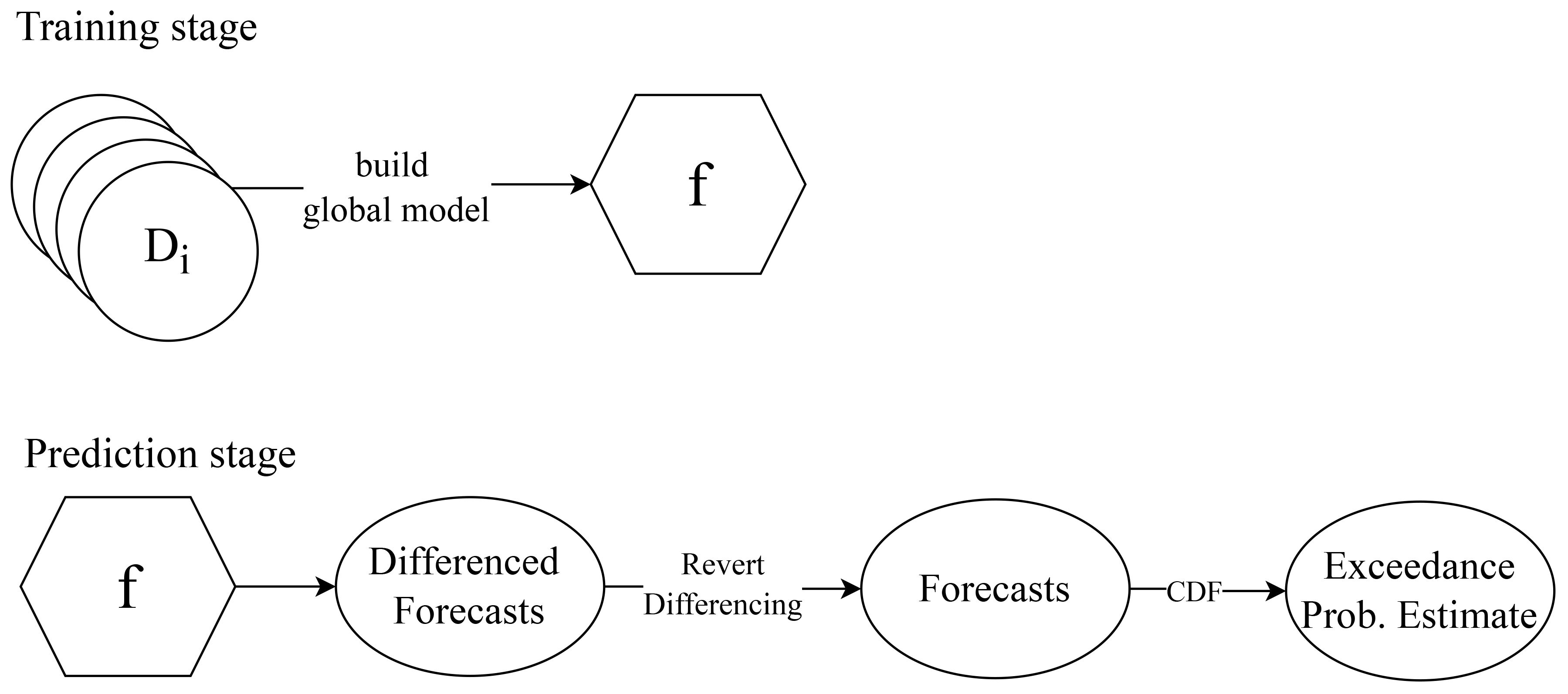
Figure 8 Training and prediction workflow.
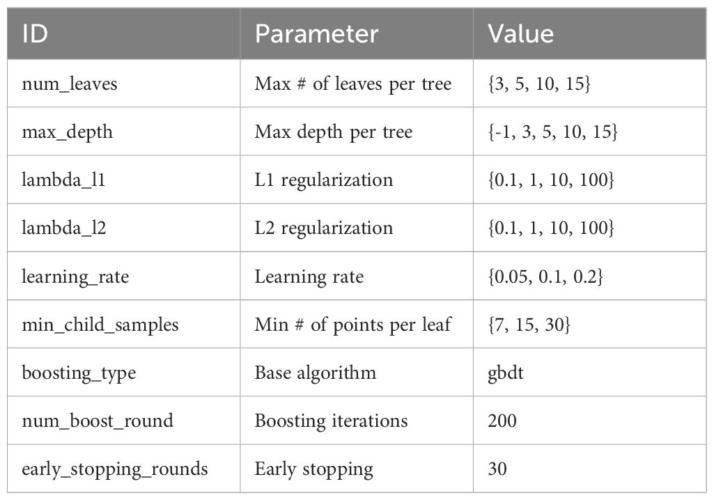
Table 3 Pool of parameters for the lightgbm.
We took a direct approach to multi-step forecasting. This means that we built a model for each forecasting horizon. This approach is a common alternative to the standard recursive method, which reuses a single model over the forecasting horizon. We prefer a direct method as it avoids the propagation of errors across the horizon (Taieb et al., 2012). After applying the model to get differenced predictions for a given time series, we revert the differencing operation to get the forecasts in the original scale.
Our goal is to forecast oxygen dynamics and predict the probability of an impending hypoxic event. Binary events such as hypoxia are usually modeled using a probabilistic binary classification model (c.f. Section 3.4). Instead, we adopt a strategy based on a forecasting model. We use the numeric forecasts for the upcoming instances to estimate the event probability according to the cumulative distribution function. In this cumulative distribution function, the location parameter of the distribution is derived from the output of the forecasting model, while the dispersion is estimated using the training data.
Let denote the forecast for a future i-th observation of oxygen concentration in a given cage produced by the lightgbm model. We assume that this prediction can be modeled using a Normal distribution with mean and standard deviation : . The standard deviation is computed using the historical observations of the corresponding cage.
In this context, we can estimate , the hypoxia probability in a given cage at the i-th time step, using the cumulative distribution function (CDF) of (Equation 2):
When evaluated at the threshold τ, the CDF represents the probability that the respective random variable will take a value less than or equal to τ. In our case, the threshold τ is equal to 7 mgL−1.
The CDF-based approach to the problem is convenient because the same forecasting model can be used to predict both the upcoming values of oxygen concentration and to estimate hypoxia probability. While probabilistic forecasts are desirable for optimal decision-making, numeric forecasts may provide valuable insights as well that help prioritize resources. From an application standpoint, the classification approach simplifies the information being given to an operator, which may help a more inexperienced user with their decision-making, while a numeric forecast offers more information, which might be useful for a more experienced operator. For example, if it is near a threshold value, the predicted trajectory offers insights into how the variable is expected to change.
Our approach also enables threshold flexibility. A standard classification approach fixes the threshold τ during training and it cannot be changed afterward. Our approach only uses the threshold during the prediction stage, so we can estimate the probability of an event at different thresholds. This can be important for farmers as the best threshold can depend on various factors, such as the number and age of fish in a cage. Overall, having access to the probabilities of an event at different thresholds might convey a better sense of the cost-benefits of available interventions.
In this section, we detail the performance estimation procedure and evaluation metrics used.
The data from different farms are collected in distinct periods, which makes it difficult to have a consistent testing period for all farms. In effect, we carried out a training and testing procedures for each fish farm where the testing period changes across these farms. For each fish farm, we set the last 40% of observations for testing. All previous observations for all farms (including the initial 60% of observations of the fish farm being tested) are compiled into a training set. The final testing periods for each fish farm are detailed in Table 4.
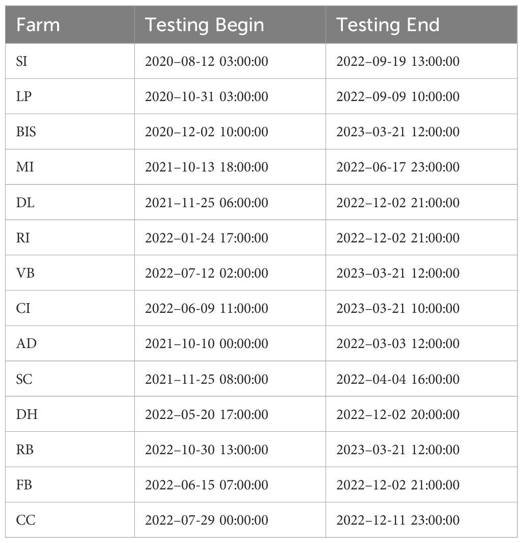
Table 4 Training and testing periods across each farm.
We also use a validation set for parameter optimization. This validation set is composed of the last 10% of observations of the training set. More precisely, the models are fit using the initial part of the training set (the initial 90% of observations of the complete training set) and evaluated in the validation set. After optimization, the model with the best parameters is then re-fit using the complete training set.
In terms of metrics, we quantify the quality of the model from different perspectives. We use the absolute error to evaluate how well the forecasts approximate the actual oxygen concentration values. We evaluate the hypoxia probability estimates using log loss. This metric quantifies how close the estimated probability is from the actual value (0 if no event occurs, or 1 otherwise).
We also evaluate the predictions made by the model from an event detection point of view. Classification problems are usually evaluated using metrics such as precision, recall, and F1-score. However, these metrics can be misleading because, as Fawcett and Provost (1999) argue, they ignore the temporal order of observations and the value of timely predictions. The main goal of our work is to detect, in a timely manner, an impending hypoxic event. In effect, we resort to the evaluation approach proposed by Weiss and Hirsh (1998) and Fawcett and Provost (1999). Specifically, we compute the event recall (ER) and the false alarm rate by unit of time (FAR). We can think of these metrics as variants of the standard recall and precision metrics but tailored for time-dependent data.
The ER metric can be defined as follows. Let T denote the total number of hypoxic events in a test dataset, and let represent the total number of those events correctly predicted by a model m. The ER for model m is given by Equation 3:
ER differs from the classical recall metrics because a single correct prediction within an observation window leading to a hypoxic event is enough to consider that the event was correctly predicted.
The idea behind ER is that multiple alarms after the first one may add no value, assuming that action is taken after the initial alarm is issued. The same argument can be made for false alarms. The classical precision metric measures the ratio of positive predictions that are correct. Similarly to recall, in a time-dependent domain, the classical precision may be misleading because multiple predictions on the same event are counted multiple times. This idea is intuited in Figure 9. This graphic shows a sequence in which predictions are being produced over time. Starting from time ti, four false alarms are triggered. Performance evaluation should take the first wrong prediction into account as a false alarm. However, the subsequent false alarms (as shown in Figure 9) are not meaningful since they add no information.
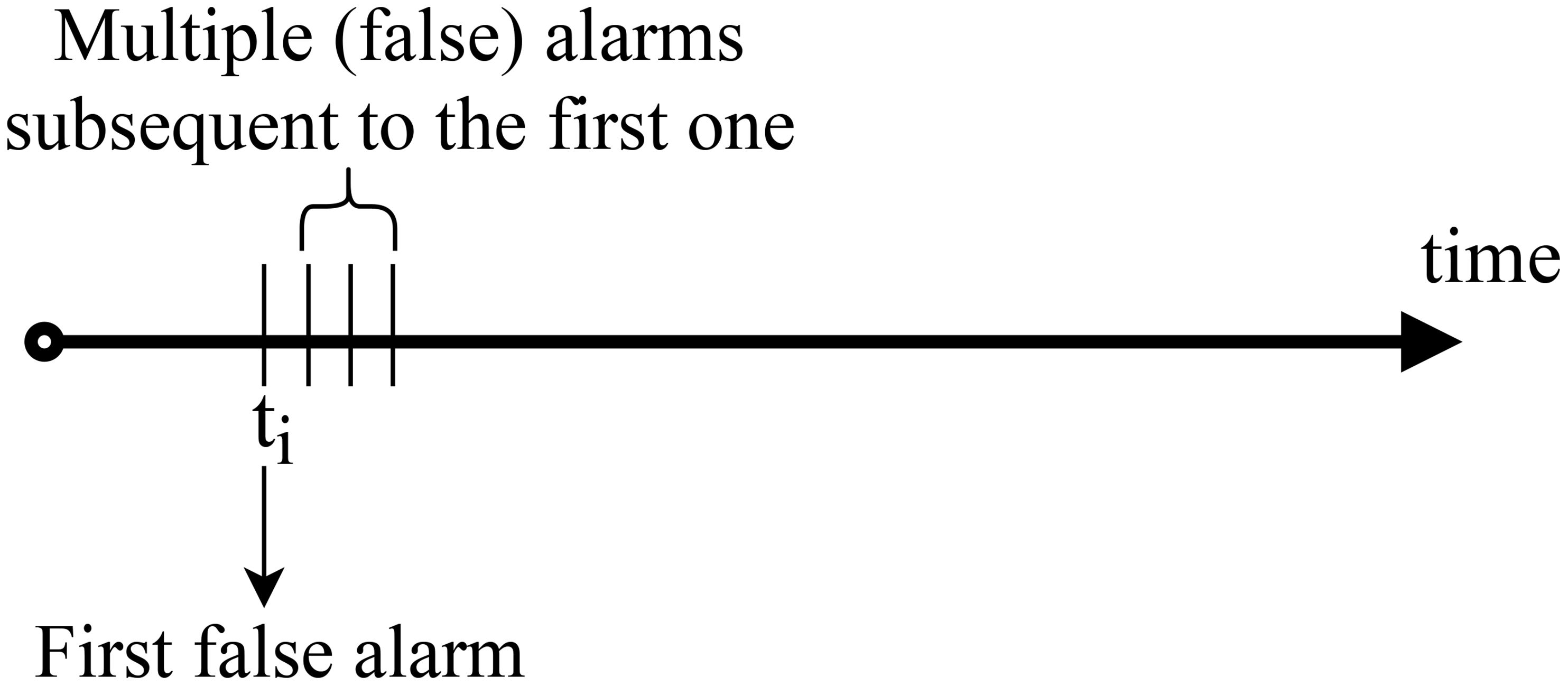
Figure 9 A sequence of consecutive false alarms. The first alarm is useful, but the subsequent ones may add no information.
We compute the FAR, which can be defined as follows. First, we compute discounted false alarms (DFA) – the number of non-overlapping observation periods associated with a wrong positive prediction. Then, we divide this number by the length of the time series. This leads to a measure of the expected number of false alarms per unit of time. In effect, the daily FAR for a model m is given by the Equation 4:
where T is the number of testing observations in the corresponding cage. We normalize the false alarm rate to a daily granularity in the interest of interpretability. This is accomplished by multiplying the original score (on an hourly basis) by 24.
Besides these metrics, we also analyze the average anticipation time of the model. That is, how long in advance the model is able to detect hypoxic events.
In this section, we present the results of the experiments. We start by illustrating the output of the model (Section 5.1) and then evaluate it from different perspectives (Section 5.2).
For illustration purposes, the model was tested on a sample cage in the LP fish farm and its predictions are shown in Figures 10, 11. Figure 10 illustrates the forecasts for the next 24 hours, along with the actual and previous values of the series. In this particular example, the model can match the actual values closely.
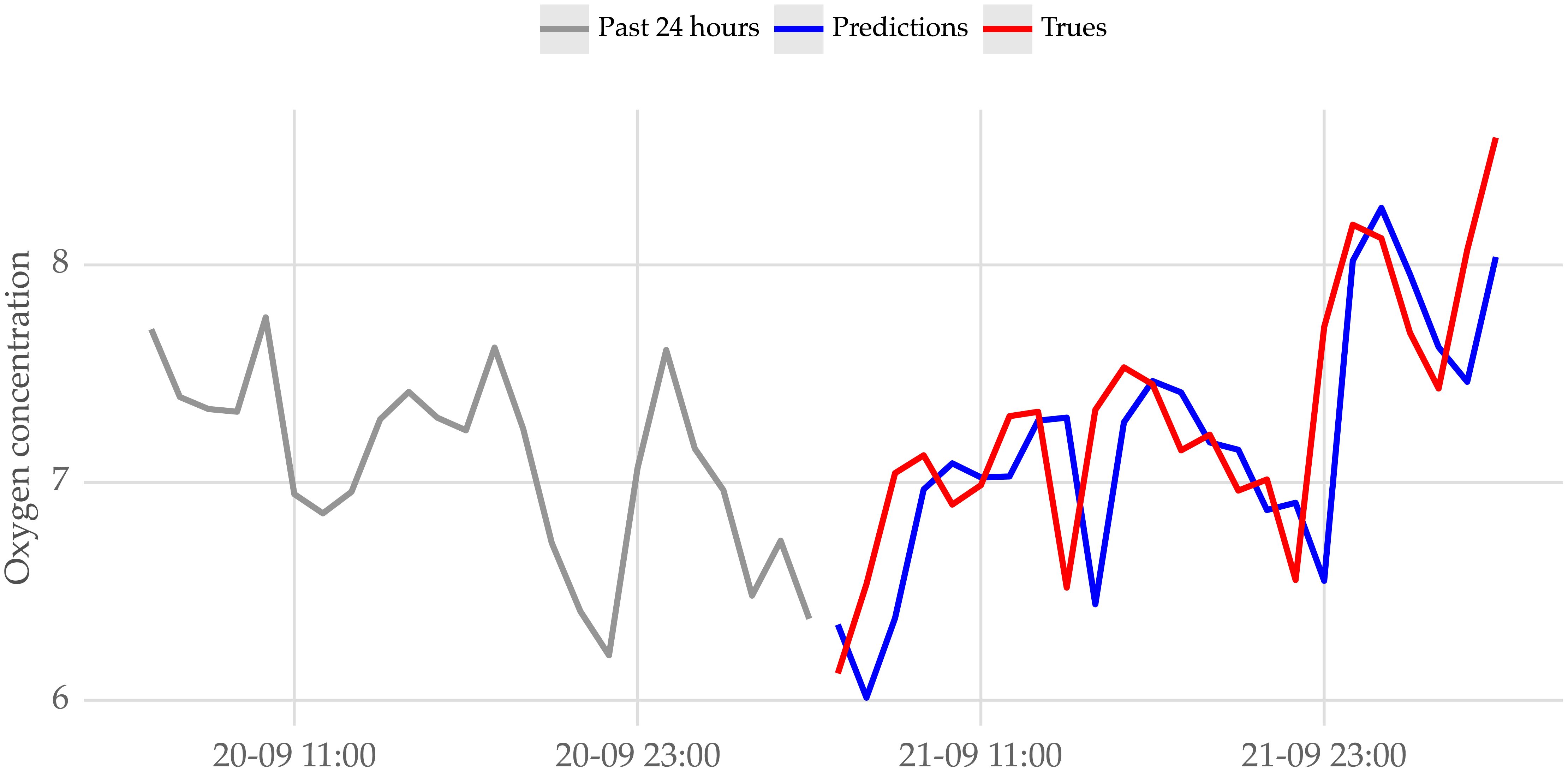
Figure 10 Sample of the forecasts for oxygen concentration, and respective true values, for a lead time of 12 hours.
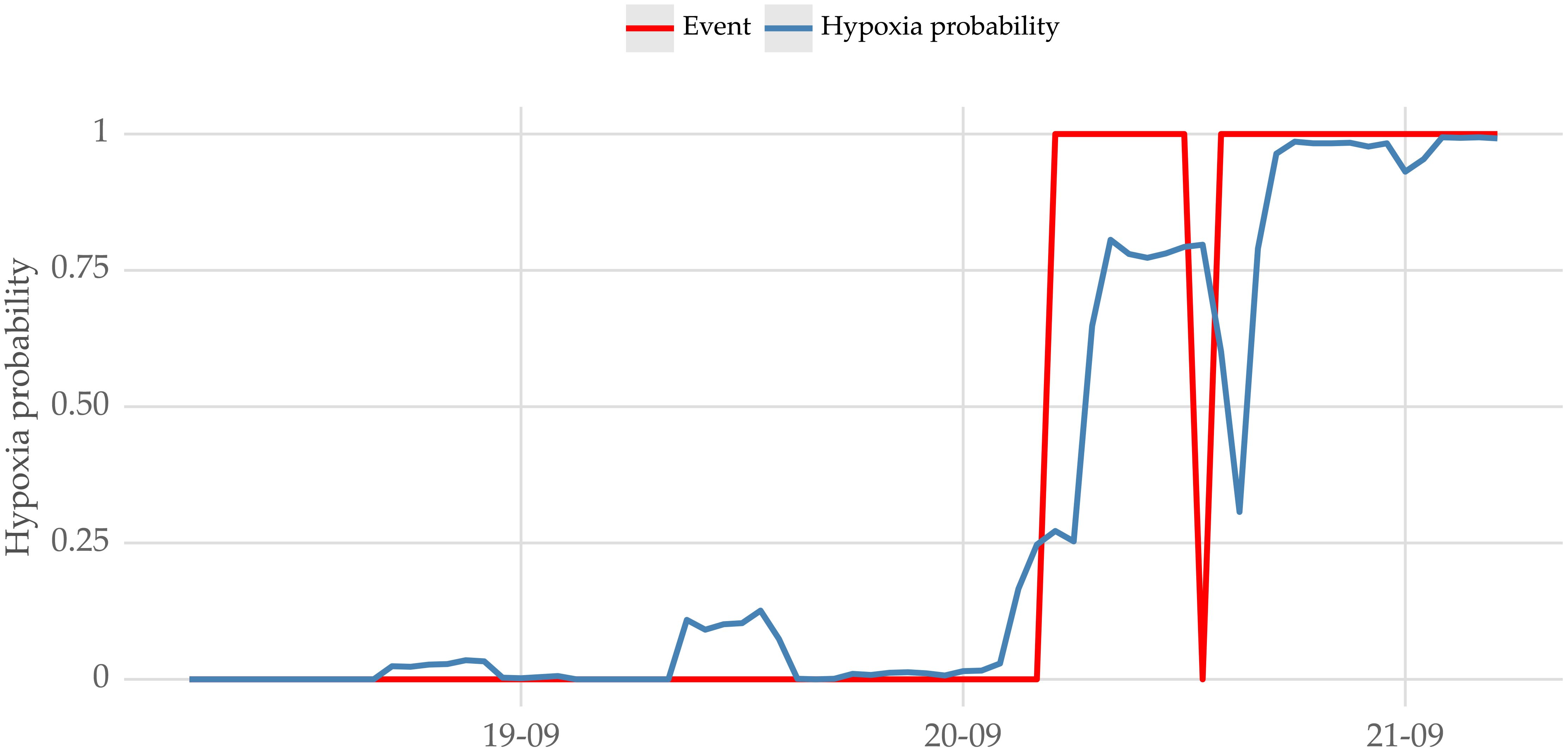
Figure 11 Sample of the forecasts for low oxygen concentration events, and respective true values. The y-axis represents the probability of hypoxia computed with a lead time of 12 hours.
Figure 11 shows the estimated probability of a hypoxic event in an example sample period. In it, a hypoxia event occurs in the final part of the sample (when the red line equals 1), and the model can detect it.
This section presents a quantitative evaluation of the model described in Section 4.
We start by comparing the developed method that leverages forecasts into exceedance probability estimates using the CDF with a probabilistic binary classification model according to the log loss. The log loss evaluates how close the probability estimates are to the actual values (0 or 1). Having accurate probability estimates is important so that farmers can assess and react to a situation in a reliable way. The classification model is trained using a lightgbm using the same procedure we used for training the forecasting model (c.f. Section 4.1.2). The only change is that the classifier is optimized for binary classification rather than regression.
The results are shown in Figure 12. Overall, the developed model (denoted as CDF) shows better performance across almost all fish farms. We conducted a Wilcoxon signed rank test, recommended by Demšar (2006), which confirmed that the difference in performance is significant.
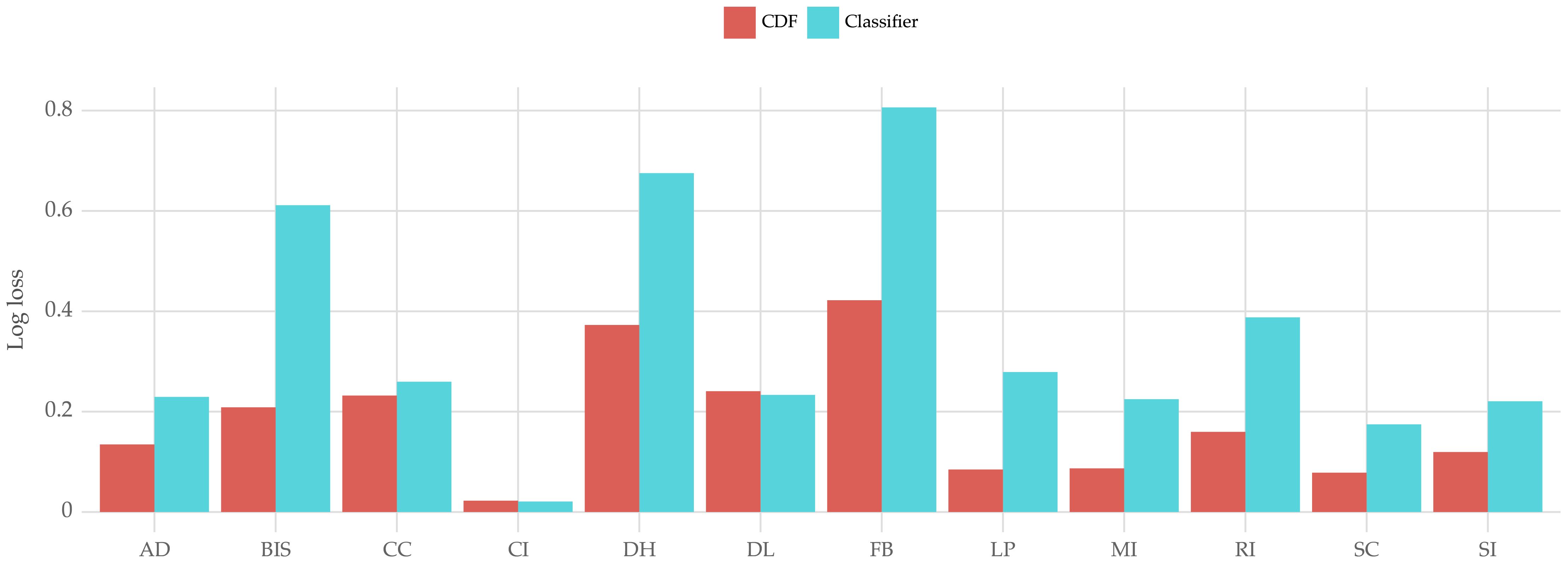
Figure 12 Log loss score across farms for the developed method (CDF) and a classification benchmark (Classifier).
Figure 13 shows the results for each farm in terms of event recall and false alarm rate, along with the number of hypoxia events that occurred during the testing period. The results vary considerably across fish farms. In some cases, the results are not representative due to the low number of events.
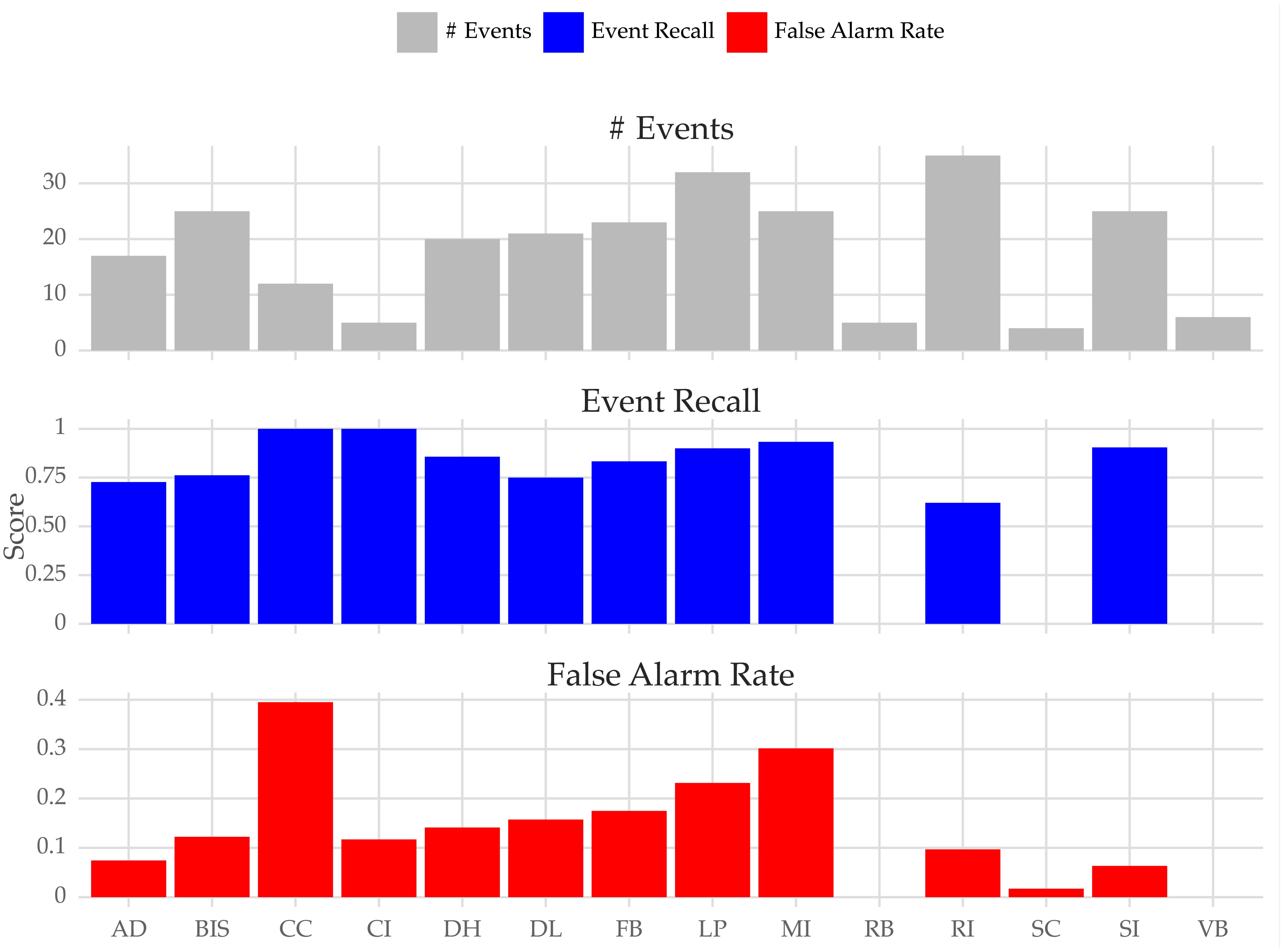
Figure 13 Number of events, event recall, and false alarm rate by fish farm.
(e.g., RB farm). For the farms with a higher number of events (e.g., LP, RI, and SI), the event recall ranges from 60% to 85%. The false alarm rate also varies across farms. For example, in the SI farm, the score is about 0.05. This means that we can expect around 5 false alarm events (sequences of false alarms) every 100 days. High scores in terms of ER are associated with either a low number of events (which means the score is not representative) or a high FAR score. The end-users can control this trade-off using the decision threshold, which in these experiments is set to 0.5. Notwithstanding, this parameter can be optimized using cross-validation.
As mentioned before, the model is designed to make predictions with a lead time of 12 hours. However, sometimes the model might detect events with some delay. Figure 14 shows the average anticipation time (in hours) for each fish farm. The results indicate that the model detects events with an anticipation time that ranges from about 5 to 8 hours.
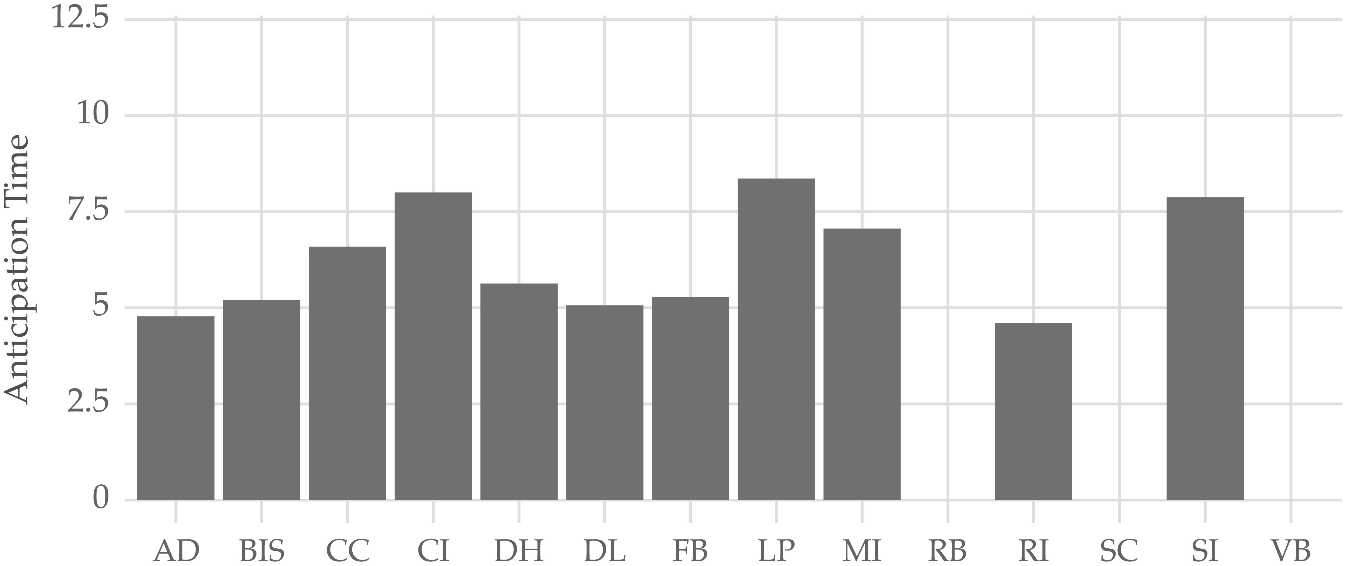
Figure 14 Average anticipation time (in hours) across all fish farms.
Finally, we also evaluated the numeric forecasts produced by the model. Figure 15 shows the distribution of absolute error (i.e., the absolute difference between the forecast and actual values) across the forecasting horizon. The median absolute error varies across farms. For example, this value is about 0.25 for the AD farm. Absolute errors above 0.5 are usually outliers (depending on the farm) according to the boxplot.
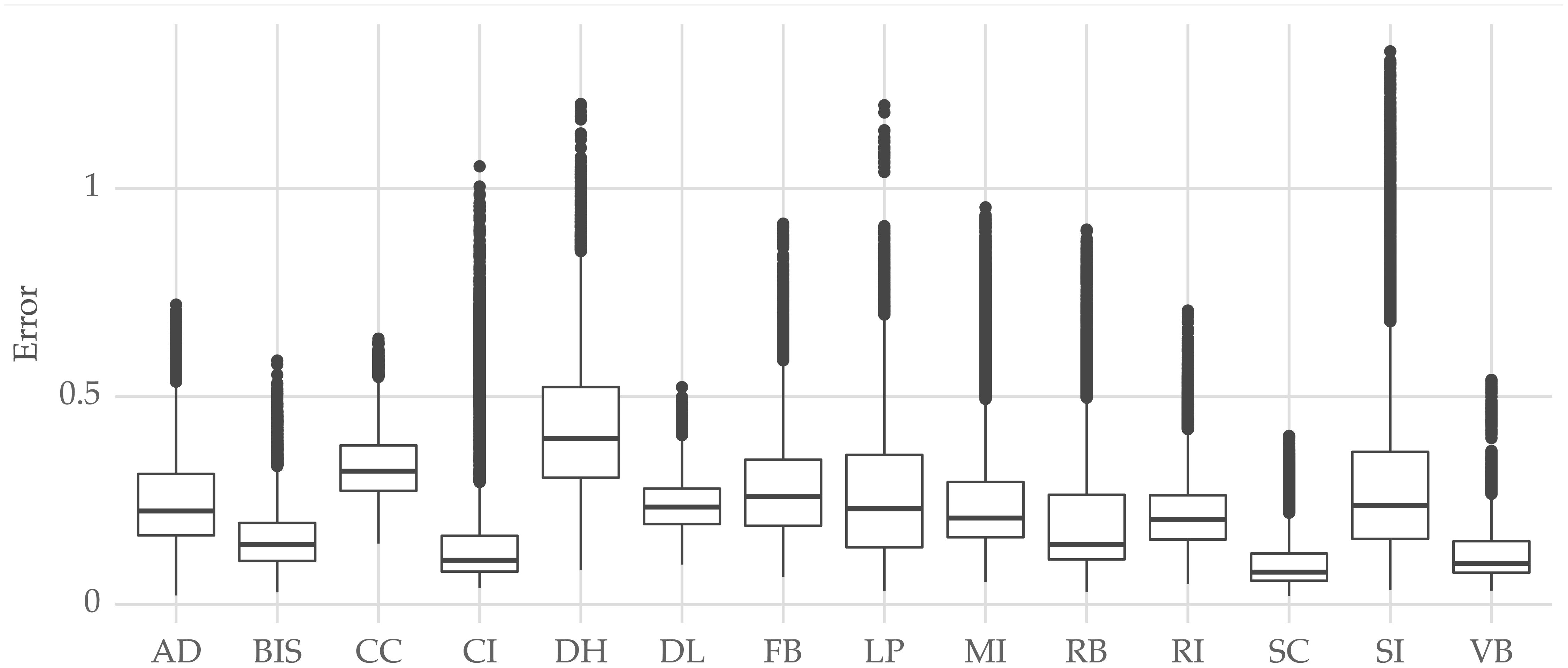
Figure 15 Distribution of absolute error across farms.
Pre-processing the data through differencing was found to be an important step in obtaining the reported forecasting performance, however, stabilizing the variance and modeling seasonal effects did not have a significant impact. We remark that, during the development of our model, we attempted to add extra meteorological and oceanographic variables. These included wind speed and direction, air temperature, solar radiation, or upwelling index. However, these did not improve forecasting performance. Another important aspect is that we average the values collected within each hour by taking the median. We adopted this approach to avoid potential anomalies due to sensor errors. However, we could also potentially have missed some brief hypoxia events that occur within each hour.
The learning algorithm applied in this work is a lightgbm that was optimized using random search. During the development stage, we attempted other algorithms, such as linear models and different types of neural networks. Overall, the lightgbm presented the best forecasting accuracy according to the metrics listed.
An important aspect of our work is that we evaluate our model based on realistic assumptions regarding its potential application. Usually, hypoxia detection models are evaluated using standard classification metrics such as precision, recall, and F1-score (e.g (Arepalli and Naik, 2024)). However, these metrics are not suitable for this problem due to the time-dependency among observations (c.f. Section 4.2.2).
The results suggest that the CDF-based approach for computing exceedance probability estimates outperforms a binary classification model. Beyond performance differences, it is important to note that the classification model is unable to produce forecasts, which are desirable in our application.
We could build two models, one regression model for forecasting and one classification model for exceedance probability estimation. However, two different models are susceptible to inconsistencies. For example, instances where the forecasts suggest a high chance of hypoxia but the classifier outputs a small probability for this event. In effect, being able to serve the two types of predictions using a single value provides consistency in the output. This can be important for a reliable use of the predictions by end-users.
There are several ways the model can be improved. We assume a constant variance when estimating the event probability using the CDF. Specifically, at each time step, we evaluate the CDF using the standard deviation of oxygen concentration of the corresponding cage computed with the whole training set. However, this statistic may vary over time, for example, due to seasonal effects. Thus, an adaptive approach (e.g., a rolling standard deviation) may lead to better probabilistic estimates.
Another point of improvement may be a better data compilation process. We apply a global approach by merging the training observations from all fish farms in a single dataset. This approach has several advantages such as the increased training sample size. This feature can be important if the user wants to deploy the model in fish farms with fewer data points available. However, introducing data from other farms may not bring value in some cases due to the idiosyncrasies of the farm. We can improve the global-local trade-off by, for example, clustering fish farms before modeling (Bandara et al., 2020).
Finally, the proposed model is based on auto-regression. We can also carry out an extended feature engineering process to improve the representation of the dataset. For example, previous works in the literature (e.g (Liu et al., 2021)) report that feature engineering based on empirical mode decomposition improves oxygen concentration forecasting accuracy.
The key role of fish farms in efficiently producing marine protein and reducing pressure on wild fish populations underscores their importance in our society. The occurrence of hypoxia episodes requires a focused approach to mitigate the potential environmental and economic impacts of these events.
In this work, we have introduced a machine learning approach aimed at forecasting oxygen concentration and detecting hypoxic events in fish farms. Our solution is based on two steps. First, we build an auto-regressive global forecasting model, utilizing historical data from multiple fish farms. Subsequently, these forecasts are transformed into hypoxia probability estimates through the CDF. The empirical results, derived from the application of the proposed model across 14 diverse fish farms, show its effectiveness in detecting hypoxia.
We identified some potential limitations of our method. One area for improvement involves the representation of the dataset used for training the model. A more comprehensive feature engineering process could enhance the accuracy of the model. Additionally, we can also explore a better trade-off between employing a local a global forecasting model.
The datasets presented in this article are not readily available because of privacy reasons. Requests to access the datasets should be directed to jennie.korus@innovasea.com.
VC: Conceptualization, Formal analysis, Investigation, Methodology, Software, Validation, Visualization, Writing – original draft, Writing – review & editing. JP: Data curation, Investigation, Software, Validation, Writing – original draft, Writing – review & editing. JK: Data curation, Resources, Writing – review & editing. FB: Data curation, Resources, Software, Writing – review & editing. JA: Software, Validation, Writing – review & editing. MO: Methodology, Validation, Writing – review & editing. AS: Project administration, Resources, Supervision, Writing – review & editing. RF: Funding acquisition, Project administration, Resources, Supervision, Writing – review & editing. JG: Funding acquisition, Project administration, Resources, Supervision, Writing – review & editing. LT: Conceptualization, Funding acquisition, Project administration, Resources, Supervision, Writing – original draft.
The author(s) declare financial support was received for the research, authorship, and/or publication of this article. This work was supported by the Atlantic Fisheries Fund project “Big Data and Precision Fish Farming in Nova Scotia” (AFF-NS-1544).
We thank Chris Whidden for taking the leadership on the project that supports this work, and Tyler Sclodnick for his valuable feedback.
Author AS was employed by the company Cooke Aquaculture Inc.
Author JK was employed by the company Innovasea Marine Systems.
The remaining authors declare that the research was conducted in the absence of any commercial or financial relationships that could be construed as a potential conflict of interest.
All claims expressed in this article are solely those of the authors and do not necessarily represent those of their affiliated organizations, or those of the publisher, the editors and the reviewers. Any product that may be evaluated in this article, or claim that may be made by its manufacturer, is not guaranteed or endorsed by the publisher.
Arepalli P. G., Naik K. J. (2024). A deep learning-enabled IoT framework for early hypoxia detection in aqua water using light weight spatially shared attention-LSTM network. J. Supercomputing. 80, 2718–2747. doi: 10.1007/s11227-023-05580-x
Bandara K., Bergmeir C., Smyl S. (2020). Forecasting across time series databases using recurrent neural networks on groups of similar series: A clustering approach. Expert Syst. Appl. 140, 112896. doi: 10.1016/j.eswa.2019.112896
Bontempi G., Ben Taieb S., Le Borgne Y.-A. (2013). “Machine learning strategies for time series forecasting,” in Business Intelligence: Second European Summer School, eBISS 2012, Brussels, Belgium, July 15-21, 2012, Tutorial Lectures 2, 62–77.
Bronco P., Torgo L., Ribeiro R. P. (2016). A survey of predictive modeling on imbalanced domains. ACM Computing Surveys (CSUR) 49, 1–50.
Burke M., Grant J., Filgueira R., Stone T. (2021). Oceanographic processes control dissolved oxygen variability at a commercial atlantic salmon farm: application of a real-time sensor network. Aquaculture 533, 736143. doi: 10.1016/j.aquaculture.2020.736143
Cerqueira V., Torgo L. (2022). Exceedance probability forecasting via regression for significant wave height forecasting. arXiv [preprint].
Cerqueira V., Torgo L., Soares C. (2022). A case study comparing machine learning with statistical methods for time series forecasting: size matters. J. Intelligent Inf. Syst. 59, 415–433. doi: 10.1007/s10844-022-00713-9
Demšar J. (2006). Statistical comparisons of classifiers over multiple data sets. J. Mach. Learn. Res. 7, 1–30.
Fawcett T., Provost F. (1999). “Activity monitoring: Noticing interesting changes in behavior,” in Proceedings of the fifth ACM SIGKDD international conference on Knowledge discovery and data mining (ACM). 53–62.
Gneiting T., Katzfuss M. (2014). Probabilistic forecasting. Annu. Rev. Stat Its Appl. 1, 125–151. doi: 10.1146/annurev-statistics-062713-085831
Godahewa R., Bandara K., Webb G. I., Smyl S., Bergmeir C. (2021). Ensembles of localised models for time series forecasting. Knowledge-Based Syst. 233, 107518. doi: 10.1016/j.knosys.2021.107518
Hai Z., Li W., Wu J., Zhang S., Hu S. (2023). A novel deep learning model for mining nonlinear dynamics in lake surface water temperature prediction. Remote Sens. 15, 900. doi: 10.3390/rs15040900
Januschowski T., Gasthaus J., Wang Y., Salinas D., Flunkert V., Bohlke-Schneider M., et al. (2020). Criteria for classifying forecasting methods. Int. J. Forecasting 36, 167–177. doi: 10.1016/j.ijforecast.2019.05.008
Khosravi A., Nahavandi S., Creighton D., Atiya A. F. (2011). Comprehensive review of neural network-based prediction intervals and new advances. IEEE Trans. Neural Networks 22, 1341–1356. doi: 10.1109/TNN.2011.2162110
Kwiatkowski D., Phillips P. C., Schmidt P., Shin Y. (1992). Testing the null hypothesis of stationarity against the alternative of a unit root: How sure are we that economic time series have a unit root? J. econometrics 54, 159–178. doi: 10.1016/0304-4076(92)90104-Y
Liu H., Yang R., Duan Z., Wu H. (2021). A hybrid neural network model for marine dissolved oxygen concentrations time-series forecasting based on multi-factor analysis and a multi-model ensemble. Engineering 7, 1751–1765. doi: 10.1016/j.eng.2020.10.023
Makridakis S., Spiliotis E., Assimakopoulos V. (2022). M5 accuracy competition: Results, findings, and conclusions. Int. J. Forecasting 38, 1346–1364. doi: 10.1016/j.ijforecast.2021.11.013
Oppedal F., Dempster T., Stien L. H. (2011). Environmental drivers of atlantic salmon behaviour in sea-cages: a review. Aquaculture 311, 1–18. doi: 10.1016/j.aquaculture.2010.11.020
Politicos D. V., Petasis G., Katselis G. (2021). Interpretable machine learning to forecast hypoxia in a lagoon. Ecol. Inf. 66, 101480. doi: 10.1016/j.ecoinf.2021.101480
Remen M. (2012). The oxygen requirement of atlantic salmon (salmo salar l.) in the on-growing phase in sea cages. (Norway: Institute of Biology, University of Bergen).
Schafer J. L., Graham J. W. (2002). Missing data: our view of the state of the art. psychol. Methods 7, 147. doi: 10.1037/1082-989X.7.2.147
Smyl S. (2020). A hybrid method of exponential smoothing and recurrent neural networks for time series forecasting. Int. J. Forecasting 36, 75–85. doi: 10.1016/j.ijforecast.2019.03.017
Subasinghe R., Soto D., Jia J. (2009). Global aquaculture and its role in sustainable development. Rev. aquaculture 1, 2–9. doi: 10.1111/j.1753-5131.2008.01002.x
Taieb S. B., Bontempi G., Atiya A. F., Sorjamaa A. (2012). A review and comparison of strategies for multi-step ahead time series forecasting based on the nn5 forecasting competition. Expert Syst. Appl. 39, 7067–7083. doi: 10.1016/j.eswa.2012.01.039
Taylor J. W., Yu K. (2016). Using auto-regressive logit models to forecast the exceedance probability for financial risk management. J. R. Stat. Society: Ser. A (Statistics Society) 179, 1069–1092. doi: 10.1111/rssa.12176
Wang X., Smith K., Hyndman R. (2006). Characteristic-based clustering for time series data. Data Min. knowledge Discovery 13, 335–364. doi: 10.1007/s10618-005-0039-x
Weiss G. M., Hirsh H. (1998). “Learning to predict rare events in event sequences,” In KDD. 98, 359–363.
White H. (1980). A heteroscedasticity-consistent covariance matrix estimator and a direct test for heteroscedasticity. Econometrica: J. Econometric Soc. 817–838. doi: 10.2307/1912934
Wild-Allen K., Andrewartha J., Baird M., Bodrossy L., Brewer E., Eriksen R., et al. (2020). Macquarie Harbour Oxygen Process model (FRDC 2016-067): CSIRO Final Report. (Hobart, Australia: CSIRO Oceans & Atmosphere). Available at: https://www.frdc.com.au/sites/default/files/products/FRDC_MH_Final_Rep_June_2020.pdf.
Yokoyama H. (1997). “Effects of fish farming on macroinvertebrates. comparison of three localities suffering from hypoxia,” in Water Effluent and Quality, with Special Emphasis on Finfish and Shrimp Aquaculture (Texas A & M University Sea Grant College Program, Bryan, TX), 17–24.
Zhang S., Wu J., Wang Y.-G., Jeng D.-S., Li G. (2022). A physics-informed statistical learning framework for forecasting local suspended sediment concentrations in marine environment. Water Res. 218, 118518. doi: 10.1016/j.watres.2022.118518
Keywords: fish farms, oxygen dynamics, hypoxia, time series forecasting, exceedance probability
Citation: Cerqueira V, Pimentel J, Korus J, Bravo F, Amorim J, Oliveira M, Swanson A, Filgueira R, Grant J and Torgo L (2024) Forecasting ocean hypoxia in salmonid fish farms. Front. Aquac. 3:1365123. doi: 10.3389/faquc.2024.1365123
Received: 03 January 2024; Accepted: 18 June 2024;
Published: 09 July 2024.
Edited by:
Prabhugouda Siriyappagouder, Nord University, NorwayReviewed by:
Clara Cordeiro, University of Algarve, PortugalCopyright © 2024 Cerqueira, Pimentel, Korus, Bravo, Amorim, Oliveira, Swanson, Filgueira, Grant and Torgo. This is an open-access article distributed under the terms of the Creative Commons Attribution License (CC BY). The use, distribution or reproduction in other forums is permitted, provided the original author(s) and the copyright owner(s) are credited and that the original publication in this journal is cited, in accordance with accepted academic practice. No use, distribution or reproduction is permitted which does not comply with these terms.
*Correspondence: Vitor Cerqueira, dmNlcnF1ZWlyYUBmZS51cC5wdA==
Disclaimer: All claims expressed in this article are solely those of the authors and do not necessarily represent those of their affiliated organizations, or those of the publisher, the editors and the reviewers. Any product that may be evaluated in this article or claim that may be made by its manufacturer is not guaranteed or endorsed by the publisher.
Research integrity at Frontiers
Learn more about the work of our research integrity team to safeguard the quality of each article we publish.