Chaos management and synchronization in the Liu financial system via sliding mode and passive control

The Liu financial dynamical system is a chaotic model that has been extensively studied for its applicability to financial and economic activities. This study examines chaos management and synchronization in this system. Two popular control techniques in non-linear system stabilization—sliding mode control (SMC) and passive control (PC)—are compared. While PC makes use of the system's passivity to accomplish control goals, SMC is made to guarantee strong synchronization in the face of external disruptions and parametric uncertainties. Lyapunov theory is used for stability analysis of both approaches, guaranteeing convergence of synchronization faults. In terms of accuracy, resilience, and computational efficiency, numerical simulations show each approach's advantages and disadvantages. The findings offer important insights into how well SMCs and PCs work to manage unpredictability in financial systems and provide valuable guidance. The results show that SMC achieves synchronization within t ≤ 1, while PC takes t ≤ 13. Maximum synchronization error in SMC reduces from 5.67 to 0.02, whereas PC reduces from 6.21 to 0.03. SMC, although faster, requires two controllers, whereas PC, using one controller, adjusts the interest rate for synchronization. These findings highlight the trade-offs in speed, complexity, and practical implementation of both methods for financial stability.

Introduction

The dynamics of economic systems are important to both macro- and microeconomics. Economic and financial systems are progressively growing intricately, and financial sectors' commercial growth varies from inadequate to vast [1]. Numerous factors have contributed to the complexity of the economic growth and expansion process. A major problem in the field of non-linear science is the study of non-linear chaotic dynamical systems [2]. The rate of inflation, the value of shares, and capital demand, along with other dynamic elements, are all part of the system [3]. A financial system can exhibit chaotic behavior, even if it has deterministic characteristics. Because of their extreme sensitivity to starting conditions, chaotic systems can take entirely different paths in response to even small mistakes. As a result, financial systems must attain chaotic stability. These characteristics are especially prominent in the Liu dynamical financial system, which offers a powerful yet simplified framework for modeling essential financial interactions. Since Lorenz's breakthrough in 1963, scientists have been very interested in studying and developing chaos [4, 5]. Numerous chaotic systems have been developed, including the Lu system [6], Chen system [7], and Rossler system [8]. Liu et al. established a system of multidimensional uncontrolled linear equations that only contained two non-linear terms [9].

Complex dynamical behaviors, such as irregularity and unpredictable long-term future behavior, are characteristics of chaotic systems. Chaos, as a complex and non-linear dynamic process, is prevalent across various fields. Current approaches to chaos control include a range of strategies intended to control and stabilize chaotic behavior in dynamical systems. Lyapunov control [10] and other non-linear control strategies are some of the notable methods. Lyapunov control is based on Lyapunov stability theory, which is concerned with establishing and ensuring the stability of non-linear systems. A Lyapunov function is used in Lyapunov control to examine and regulate the dynamics of a system. Sliding mode control is a straightforward method for managing chaos that has been successfully used in uncertain systems and control non-linear systems. Russian scientists developed variable structure control, also called sliding mode control, in the early 1960s and later documented it in Utkin's monograph in the 1970s [11]. Since then, SMC has been extensively studied and effectively used to solve a wide range of real-world problem areas because of its ease of implementation and adaptability in responding to system fluctuations and uncertainty [12]. SMC's sliding motion is its most appealing feature. When in the sliding mode, the system's fluid movement is effectively restricted to a certain region of the entire state space. Therefore, adopting an appropriate feedback control method to explore and evaluate chaos management and synchronization is currently my main area of interest. The stability, sliding mode control [13], passive control [14], and synchronization of the Liu financial dynamical system are all explored in this study.

A simplified depiction of reality, an economic model, is intended to produce testable hypotheses regarding economic activity. An essential characteristic of an economic model is that it is inherently subjective in its creation due to the lack of objective metrics for economic results. To better comprehend this intricate dynamic of these systems, several financial and economic models have been put out in the literature since Strotz et al. [15, 16] discovered chaos in an economic model. Several models are available, including the new hyperchaotic finance model [17], the Investment Saving-Liquidity Money (IS-LM) model [18], the forced Van der Pol model [19], and numerous others. An extremely intriguing model to depict the dynamics of financial systems was put forth by Ma and Chen in 2001 [20]. An intense sensitivity to the initial circumstances of the system's variables and parameters was also discovered by the model's analysis, along with some intriguing dynamics. Several financial variables, including the exchange rate, Gross Domestic Product (GDP), interest rate, and production, have memory, meaning that any upcoming changes in these variables are impacted by current and historical changes.

Furthermore, in 2020, Liao et al. [21] introduced a new model to enhance comprehension of financial system dynamics. This novel model considers the fact that investment demand influences the price index, in contrast to the approach put out by Ma and Chen [3]. It was discovered that this financial system's complex behavior is the consequence of three components interacting with one another. In financial systems, chaotic behavior is undesirable because it makes economic and financial predictions difficult and, as a result, increases investment risk. Hereafter, it is managed in the presence of uncertainty pertaining to the system parameters.

In financial systems, chaos control has been extensively researched in the literature. Numerous methods have been developed to manage chaotic financial systems. One of the other well-known control techniques is sliding mode control, whose dynamic performance is dictated by the specified manifold or sliding surface where control is maintained by a switching structure [22]. This technique forces the system states to remain on the sliding surface, resulting in discontinuous control. Due to its significant impact on lowering complexity and expense, synchronization is now best implemented using a single-state controller. Because it only requires one controller, the passive control approach has been becoming more and more popular for synchronizing and managing chaotic systems. The primary goal of passivity theory is to maintain system stability by putting in place a controller that makes the closed-loop system passive upon the characteristics of the system. The passive control approach has been effectively used in recent years to synchronize hyperchaotic Lorenz systems [14], chaotic systems such as Rikitake [23], unified [24], and others. Since passive control does not depend on exact real-time changes, it ensures robust stability even in the face of modeling uncertainties and external disturbances. Numerous studies have examined the sliding mode and passive control methodologies [14, 22–24]. Some unstable financial systems have been introduced in the past 10 years. The topological structure, stability, equilibrium points, and Lyapunov exponents are examples of the dynamic behaviors of chaotic finance systems, including a detailed investigation of Hopf bifurcation analysis [25]. Using linear feedback control and efficient speed feedback control [17], chaotic financial systems were brought under control through approaches such as adaptive control [26], passive control [27], time-delayed feedback control [28], the choice of gain matrix control [29], and the revision of gain matrix control [29]. It has been demonstrated that a fractional-order chaotic finance system can be regulated by employing a sliding mode control technique [30], along with approaches such as nonlinear feedback controllers [2], adaptive controllers [31], and active controllers [32], and a single controller based on Lyapunov stability theory. The chaotic finance systems are synchronized using linear matrix inequality [33].

Despite the extensive studies on chaotic economic systems, including the Lorenz [34], Lu [35], Chen [36], and Rossler systems [37], limited research has focused on the Liu [38] financial dynamical system—a system with complex non-linear interactions relevant to financial modeling. While various chaos control methods, such as Lyapunov control and passive control [27], have been employed in different financial systems, there is still a lack of robust control strategies specifically designed for the Liu system. In addition, chaos synchronization in financial systems is crucial for stability, yet most existing studies have not explored the combined effects of stability analysis, sliding mode control (SMC), and synchronization in the Liu system under various conditions of uncertainty. In this study, we examine the robust regulation of this chaotic behavior and the chaos in the financial system as described by the Liu dynamical system [38, 39], which is motivated by the discussions above. To address this instability, the study proposes sliding mode control (SMC) as a robust method for stabilizing chaos, ensuring the system remains resilient against uncertainties. The primary benefit of SMC is its ability to change the control law, which forces the system's states from their initial states onto a predetermined sliding mode surface [40]. The system on the sliding mode surface has desirable characteristics, including quick response, low sensitivity to outside noises, robustness to system uncertainties, easy realization, and so forth. Around this sliding surface, SMC produces a discontinuous control law and limited switching [41]. Consequently, this sliding surface is bound to determine the direction of the state variables' motion and the dynamics of the system. However, the existence of such a control law leads to an undesirable issue with sliding control, namely the “chattering phenomenon,” which should be reduced or eliminated in some way. However, the existence of such a control law leads to an undesirable issue with sliding control, namely, the “chattering phenomenon,” which should be reduced or eliminated in some way. The literature has proposed a number of methods, most of which are predicated on the continuous approximation of the discontinuous sign function. A sliding mode controller's design consists of the following:

1) Use a “sliding surface” that is robust during the reaching phase and depicts the “desired stable dynamics”.

2) The “control law” that ensures “the sliding condition” and “the reaching condition” is described.

In addition, the research explores synchronization between the two Liu financial systems, which is crucial for maintaining coherence in financial behavior and stability. A comparative study evaluates the effectiveness of Lyapunov control, passive control, and SMC, identifying the most suitable approach for managing chaos in financial dynamics. Furthermore, the study validates its theoretical findings through extensive numerical simulations, including time response analysis, phase portraits, and synchronization error dynamics, demonstrating the practical applicability of the proposed control methods. By addressing these key aspects, this research advances non-linear financial modeling and offers an effective approach to managing chaos in economic systems, ultimately contributing to improved financial stability.

This article's remaining sections are organized as follows: In Section 2, the Liu financial dynamical system is introduced, and its governing equations are discussed. The system's parameters and their economic interpretations are also provided. In addition, the chaotic behavior of the Liu system under specific parameter conditions is analyzed. Section 3 focuses on the synchronization of the Liu dynamical system using sliding mode control (SMC). The design of the SMC strategy is presented, followed by a stability analysis based on Lyapunov theory. The effectiveness of the proposed control scheme in achieving synchronization is demonstrated. In Section 4, the organization of the Liu financial system via passive control (PC) is explored. The principles of passive control are introduced, and a control law is designed to stabilize the system. Theoretical justifications for stability are provided, along with a comparison between SMC and PC strategies. Section 5 presents numerical simulations to validate the proposed control methods. The time response, phase portraits, and error dynamics are illustrated to confirm the effectiveness of the applied controllers. A comparative analysis between different control strategies is also included. Finally, Section 6 concludes the article with a summary of key findings, highlighting the contributions of the study. Future research directions, including adaptive control techniques and further applications in financial modeling, are also discussed.

Liu financial dynamical system

To foster economic growth and commercial demand through investment, a financial system's organizational units and exchanges usually connect in a complex way. Three state variables' temporal variation has been identified by the economic model considered in this study: Let x represents the price index or market price, y represents the interest rate or inflation rate, and z represents the investment demand or capital. The price exponent determines the variance in price distribution. The quantity that the lender pays the borrower to utilize assets, represented as an amount of capital, is known as the rate of return. The desired or expected capital and inventory of an organization is known as expenditure demand, and it is negatively correlated with financing rates and investment costs. The Liu financial dynamical system is described by a set of three first-order differential equations as follows [39]:

$\begin{array}{r}\dot{x}=a(y-x)\\ \dot{y}=bx-dxz\\ \dot{z}=-cz+f{x}^2& (1)\end{array}$

where a, b, c, d, and f are all beneficial constant parameters that, respectively, describe the quantity of savings, the cost per savings, the elasticity of economic demand, the influence of the cross-market, and the growth factor of investments [46]. A fiscal system's savings level shows that the enterprise unit's overall economic expansion has accelerated. The quantity of distribution from objective investments that is obtained without initial expense is defined as the per-investment cost. The relationship between the cost of a good change and alterations in the quantity demanded is known as advertising demand elasticity. Cross-market influence means the impact of interactions across different markets or sectors, such as how the behavior in one market (supply or demand) influences another. The growth factor of investments means a growth or amplification factor in the system, representing how investments fuel further expansion, potentially due to compounding effects or returns. When a = 10, b = 40, c = 2.5, f = 4, and d = 1, the dynamic financial system behaves chaotically [38]. Figure 1 displays the chaotic financial system's timing response with the initial circumstances: x(0) = 10, y(0) = 20, and z(0) = 90. Figure 2 displays the 2D phase portraiture, Figure 3 displays the 3D phase plane, and Figure 4 displays the error states' time response before synchronization.

Figure 1

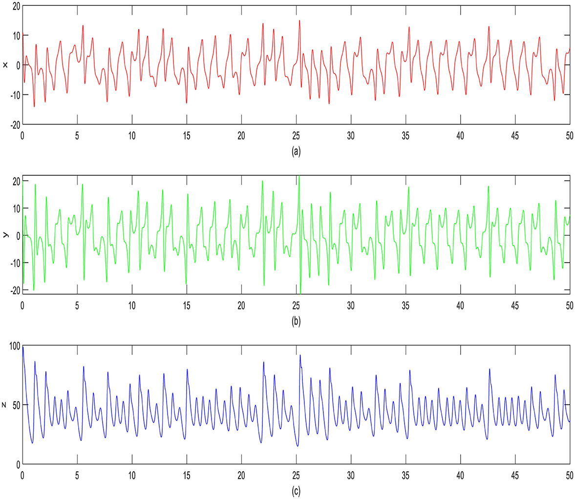
Figure 1. Chaos finance system time signals x, y, and z prior to synchronization for (a) x signals, (b) y signals, and (c) z signals.

Figure 2

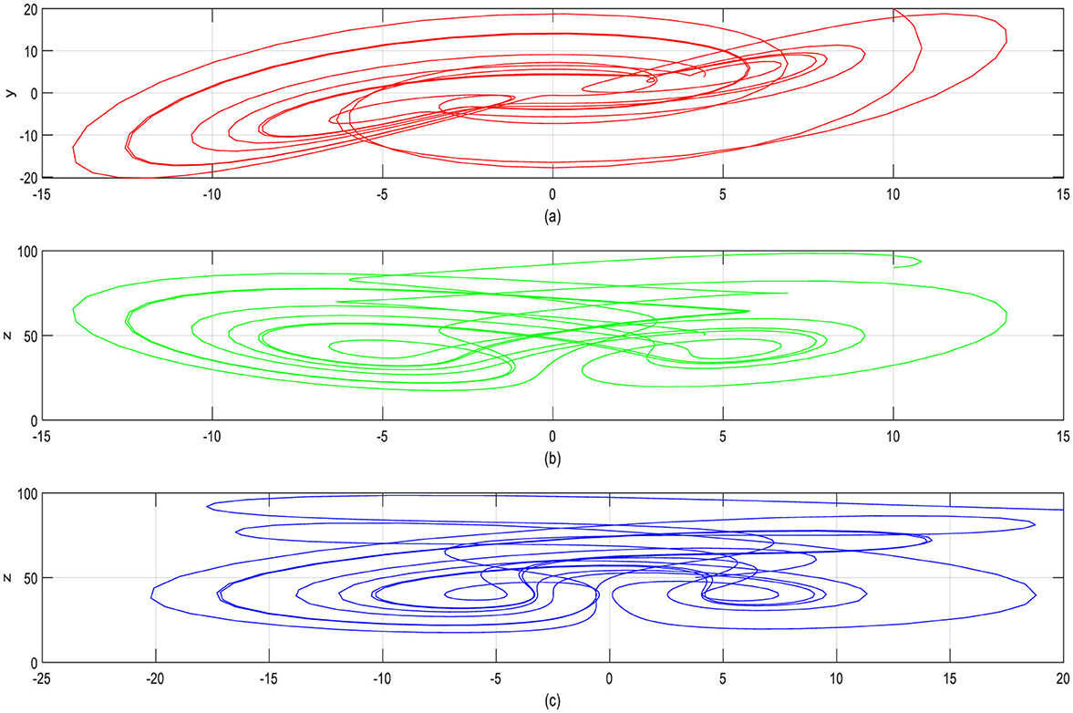
Figure 2. Phase depicts a chaotic financial system in three different planes: (a) x-y, (b) y-z, and (c) z-x.

Figure 3

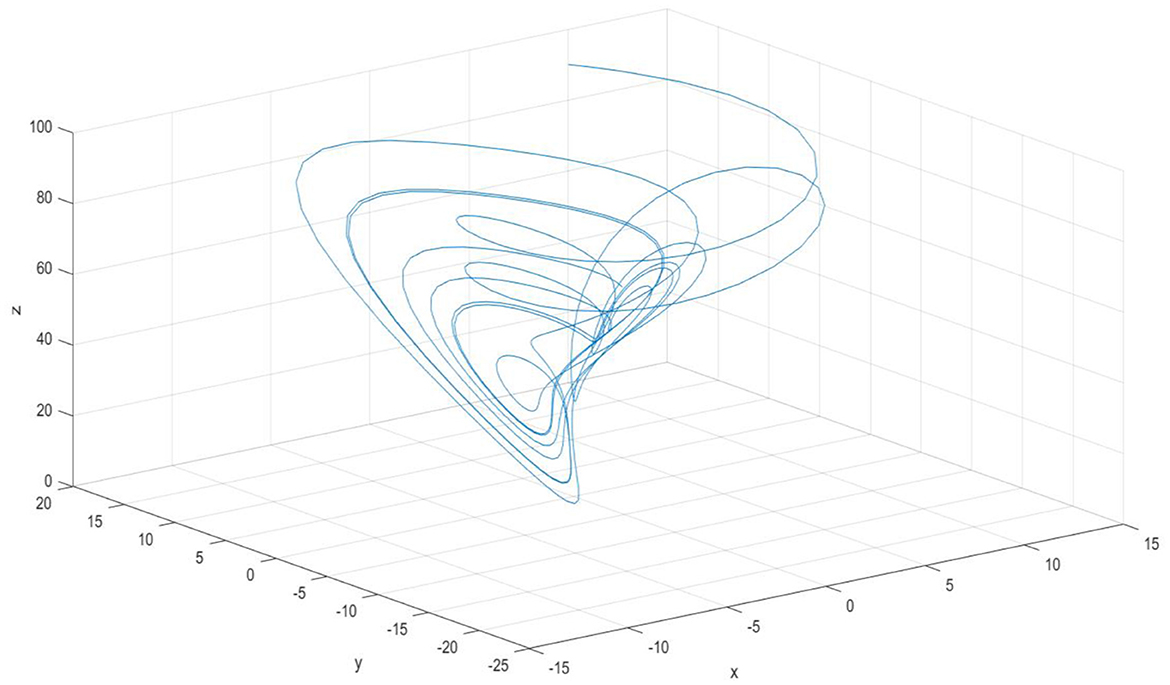
Figure 3. Chaotic finance system's three-dimensional phase plane.

Figure 4

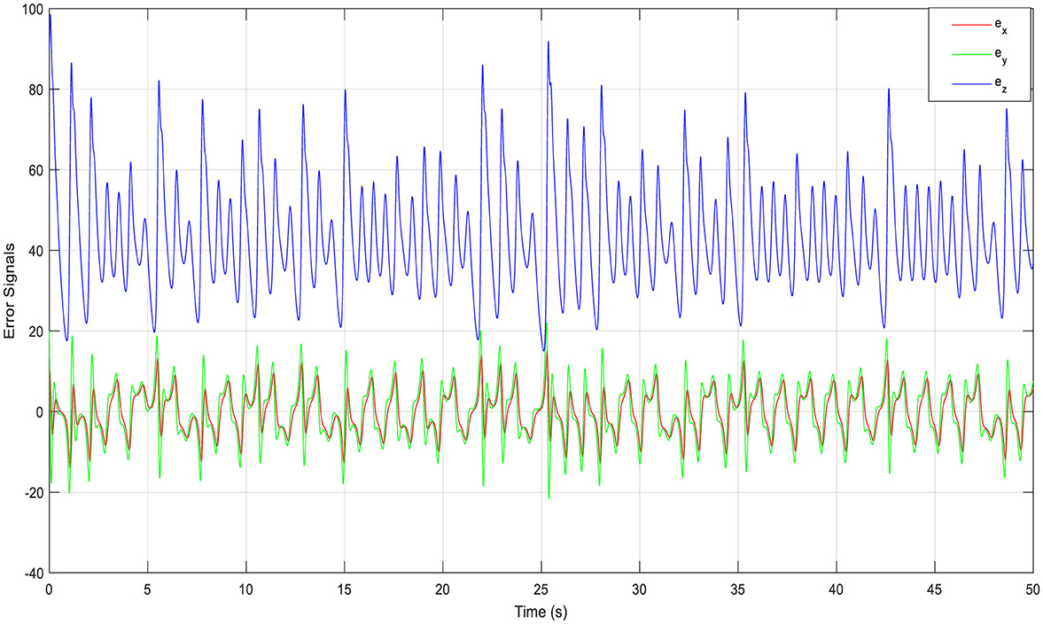
Figure 4. Interval retort of the error states before synchronization.

The synchronization of the Liu dynamical system applying SMC

The boundaries a, b, d, c, and f are taken within a limit to make sure that the system (Equation 1) will demonstrate changeable behavior. It is expected that two chaotic financial systems, with the drive system controlling the response system, are used to observe the synchronization. Subtitles 1 and 2 stand for the drive system and response system, respectively. The drive system is provided by

$\begin{array}{r}{\dot{x}}_1=a(y_1-x_1)\\ {\dot{y}}_1=b{x}_1-d{x}_1{z}_1\\ {\dot{z}}_1=-c{z}_1+f{x_1}^2& (2)\end{array}$

and the response system is described as

$\begin{array}{r}{\dot{x}}_2=a(y_2-x_2)+u_1(t)\\ {\dot{y}}_2=b{x}_2-d{x}_2{z}_2+u_2(t)\\ {\dot{z}}_2=-c{z}_2+f{x_2}^2+u_3(t)& (3)\end{array}$

where u₁(t), u₂(t), and u₃(t) in Equation 3 are to be formed. To determine the control capabilities for time, the drive system is eliminated from the reaction time system. The state errors e₁, e₂, and e₃ are to be controlled, and the controlling system (Equation 2) is expressed as

$\begin{array}{l}{e}_1=x_2-x_1\\ e_2=y_2-y_1\\ e_3=z_2-z_1& (4)\end{array}$

Thus, the patterns of errors become

$\begin{array}{r}{\dot{e}}_1=a{e}_2-a{e}_1+u_1(t)\\ {\dot{e}}_2=b{e}_1-d(x_2{z}_2-x_1{z}_1)+u_2(t)\\ {\dot{e}}_3=-c{e}_3+f({x_2}^2-{x_1}^2)+u_3(t)& (5)\end{array}$

In matrix notation, we can normalize the error behavior (Equation 5) to

$\begin{array}{ll}\dot{e}=Ae+\eta (x,y)+u& (6)\end{array}$

where,

$\begin{array}{r}A=\left[\begin{array}{ccc}-a& a& 0\\ b& 0& 0\\ 0& 0& -c\end{array}\right],\eta \left(x,y\right)=\left[\begin{array}{c}0\\ -d(x_2{z}_2-x_1{z}_1)\\ f({x_2}^2-{x_2}^2)\\ \end{array}\right]\\ u=\left[\begin{array}{c}{u}_1(t)\\ u_2(t)\\ u_3(t)\end{array}\right]& (7)\end{array}$

The meaning of the control signal u established on the sliding mode control methodology is as follows [42]:

$\begin{array}{ll}u(t)=-\eta \left(x,y\right)+ℬv\left(t\right)& (8)\end{array}$

where B is a matrix and v is a control signal. To make (A, B) controllable, B was selected.

Consequently, B is interpreted as

$\begin{array}{ll}B=\left[\begin{array}{c}1\\ 0\\ 1\\ \end{array}\right]& (9)\end{array}$

Substituting Equation 8 into Equation 7, the error behavior simplifies to

$\begin{array}{ll}\dot{e}=Ae+Bv& (10)\end{array}$

It has a single input, v, and is a proportional time-dependent control scheme.

The initial global chaotic synchronizing question can be converted into an analogous problem of stabilizing the system's zero-solution e = 0 in Equation 10, provided that an appropriate sliding mode control is selected. The switchable mode control defines the variable.

$\begin{array}{ll}s(e)=Ce=c_1{e}_1{c}_2{e}_2+\dots \dots \dots \dots \dots \dots +c_n{e}_n.& (11)\end{array}$

as, C = [c₁ c₂………c_n] is a coefficient trajectory that needs to be formed.

Now reduce the system (Equation 10) motion in the sliding mode control to the sliding manifold denoted by s = {xϵRⁿ, |s(e)| = 0}

which must remain unchanged under the influence of the error dynamics described in Equation 10. When the sliding manifolds, the system (Equation 10) fulfills the following requirements:

$\begin{array}{ll}s(e)=0& (12)\end{array}$

It becomes a series of defining Equations and

$\begin{array}{ll}ṡ(e)=0& (13)\end{array}$

In the chaotic case, the parameter values are a = 10, b = 40, c = 2.5, f = 4, and d = 1.

The variable for the sliding mode is chosen as

$\begin{array}{l}S=Ce=[20-1]e=2e_1-e_3.\end{array}$

which ensures that the sliding mode state Equation is asymptotically stable.

Select the sliding mode gain as follows: K = 5 and q = 0.1.

A high value of K can lead to chattering, while a suitable rate of q is selected to both accelerate the time it takes to accomplish the sliding manifold and minimize system chattering. Using Equations 10, 11, the Equation 13 can be changed as

$\begin{array}{ll}ṡ(e)=C(Ae+Bv)& (14)\end{array}$

According to the sliding mode control theory's property [42],

$\begin{array}{ll}v\left(t\right)=-{(CB)}^{-1}[C\left(KI+A\right)e+qsign(s)& (15)\end{array}$

where C is chosen such that CB ≠ 0

Now, the v(t) control signal becomes

$\begin{array}{ll}v(t)=-10e_1+20e_2-2.5e_3+0.1sign(s)& (16)\end{array}$

As a result, the necessary sliding mode controller is acquired as [42]

$\begin{array}{ll}u=-\eta (x,y)+Bv& (17)\end{array}$

Then, the required sliding mode control signal is obtained as Equation 8, where η(e) and B are described as in Equations 7, 9, respectively:

$\begin{array}{r}{u}_1(t)=0\\ u_2(t)=d(x_2{z}_2-x_1{z}_1)+v(t)\\ u_3(t)=-f({x_2}^2-{x_1}^2)+v(t)& (18)\end{array}$

Equations 16, 17 complete the synchronization of the Liu system (Equation 3) using the sliding mode control approach. Therefore, two equal Liu systems work together using sliding mode control.

Theorem 3.1. For all initial conditions x(0), y(0) ∈ Rⁿ, the sliding mode control law guarantees that the drive system (Equation 2) and the response system (Equation 3) are globally and asymptotically synchronized.

$\begin{array}{ll}u(t)=-\eta (x,y)+Bv(t)& (19)\end{array}$

where B is a column vector such that (A, B) is controllable and v(t) is defined by Equation 15. Furthermore, k and q, the sliding mode gains, are positive.

Proof. First, observe that the closed-loop dynamics can be achieved by substituting Equations 19, 17 into the error dynamics (Equation 7).

$\begin{array}{ll}\dot{e}=Ae-B{(CB)}^{-1}[C(KI+A)e+qsgn(s)]& (20)\end{array}$

To demonstrate that the error dynamics (Equation 20) is globally stable over time, let us examine the proposed Lyapunov function that the Equation depicts.

$\begin{array}{ll}v(e)=\frac{1}{2}{s}^2(e)& (21)\end{array}$

which is a positive definite function on Rⁿ.

Differentiating v along the trajectories of Equation 20 or the equivalent dynamics (Equation 14), we obtain

$\begin{array}{ll}\stackrel{.}{v}(e)=s(e)ṡ(e)=-k{s}^2-qsgn(s)& (22)\end{array}$

which is a negative definite function on Rⁿ.

The error dynamics (Equation 20) is therefore immediately globally asymptotically stable for all initial conditions e(0)ϵRⁿ, according to the Lyapunov equilibrium principle.

This concludes the documentation.

The organization of Liu systems via passive control (PC)

At this point, the system that drives will continue to be [43]

$\begin{array}{r}{\dot{x}}_1=a(y_1-x_1)\\ {\dot{y}}_1=b{x}_1-d{x}_1{z}_1\\ {\dot{z}}_1=-c{z}_1+h{x_1}^2& (23)\end{array}$

and the system for reporting is provided by

$\begin{array}{r}{\dot{x}}_2=a(y_2-x_2)+u(t)\\ {\dot{y}}_2=b{x}_2-d{x}_2{z}_2\\ {\dot{z}}_2=-c{z}_2+h{x_2}^2& (24)\end{array}$

where the passive control function to be found is u(t) in Equation 24. The timing error is obtained by subtracting the drive system from the response system, similar to the sliding mode control. Then,

$\begin{array}{r}{\dot{e}}_1=a{e}_2-a{e}_1+u(t)\\ {\dot{e}}_2=b{e}_1-d{x}_2{z}_2+d{x}_1{z}_1\\ {\dot{e}}_3=-c{e}_3+h({x_2}^2-{x_1}^2)& (25)\end{array}$

where the system (Equation 25) is referred to as the error system, and e₁, e₂, and e₃ are the actual errors. System (Equation 25) has a word that may be expressed as

$\begin{array}{ll}{x_2}^2-{x_1}^2=(x_2+x_1)e_1& (26)\end{array}$

So, the error system (Equation 25) can be rewritten in the following form:

$\begin{array}{r}{\dot{e}}_1=a{e}_2-a{e}_1+u(t)\\ {\dot{e}}_2=b{e}_1-d{x}_2{z}_2+d{x}_1{z}_1\\ {\dot{e}}_3=-c{e}_3+h{e}_1(x_2+x_1)& (27)\end{array}$

To stabilize the error system (Equation 27) at zero equilibrium, the passive controllers u(t) must be found.

By assuming that the state variable e₁ is the output of the system and supposing $Y=e_1,z_1=e_2,z_2=e_3,z={\left[z_1,z_2\right]}^T$, the system (Equation 27) can be denoted by normal form:

$\begin{array}{r}{Ż}_1=bY-d{x}_2{z}_2+d{x}_1{z}_1\\ {Ż}_2=-c{e}_3+hY(x_2+x_1)\\ Ẏ=a{z}_1-aY+u(t)& (28)\end{array}$

The modified iteration of the passive control theory is as follows:

$\begin{array}{r}Ż=f_0(Z)+p(Z,Y)Y,\\ Ẏ=b(Z,Y)+a(Z,Y)u,\end{array}$

and according to system (Equation 28):

$\begin{array}{r}{f}_0\left(Z\right)=\left[\begin{array}{c}-d{x}_2{z}_2+d{x}_1{z}_1\\ -c{z}_2\\ \end{array}\right],\\ p(Z,Y)=\left[\begin{array}{c}b\\ h(x_2+x_1\end{array}\right],\\ b\left(Z,Y\right)=a{Z}_1-aYa\\ \left(Z,Y\right)=1& (29)\end{array}$

where $W(Z)=\frac{1}{2}({z_2}^2+{z_2}^2)$ is a Lyapunov function of $f_0\left(Z\right)$ with W(0) = 0. Then,

$\begin{array}{r}\frac{d}{dt}V(Z,Y)=\frac{\partial W(Z)}{\partial Z}Ż+YẎ\\ =\frac{\partial W(Z)}{\partial Z}{f}_0(Z)+\frac{\partial W(Z)}{\partial Z}p(Z,Y)Y+Yb(Z,Y)u& (30)\end{array}$

According to Equation 29, by taking the derivative of W(Z)

$\begin{array}{r}Ẇ(Z)=\frac{d}{dt}W(z)=\frac{\partial W(Z)}{\partial Z}{f}_0(Z)=\left[Z_1{Z}_2\right]\left[\begin{array}{c}-d{x}_2{z}_2+d{x}_1{z}_1\\ -c{z}_2\\ \end{array}\right]\\ =\left[\begin{array}{c}-d{x}_2{z}_1{z}_2+d{x}_1{z_1}^2\\ -c{z_2}^2\\ \end{array}\right]& (31)\end{array}$

Since W(Z) ≥ 0 and Ẇ(Z) ≤ 0, it can be decided that W(Z) is the Lyapunov function of f₀(Z) and that f₀(Z) is globally asymptotically stable. The controlled system (Equation 27) is equivalent to a passive system and can be asymptotically globally stabilized at its zero equilibrium by the following state feedback controller:

$\begin{array}{r}u(t)=a(Z,Y{)}^{-1}\left[-b^T(Z,Y)-\frac{\partial W(Z)}{\partial Z}p(Z,Y)-\alpha Y+v\right]\\ =1^{-1}[-(a{z}_1-aY)-[z_1{z}_2]\left[\begin{array}{c}b\\ h(x_1+x_2)\end{array}\right]-\alpha Y+v]\\ =aY-(a+b)z_1-h(x_1+x_2)z_2-\alpha Y+v& (32)\end{array}$

where v is an external input signal and α is a positive constant. Z₁ = e₂, Z₂ = e₃, and Y = e₁ conversions are noted, and the passive control function turns into

$\begin{array}{ll}u(t)=a{e}_1-(a+b)e_2-h(x_1+x_2)e_3-\alpha e_1+v& (33)\end{array}$

Equation 33 completes the synchronization of the chaotic finance system (Equation 24) using the passive control method. As a result, two identical chaotic finance systems are synchronized through passive control.

The theory of passive control

Consider the following differential Equation:

$\begin{array}{ll}\{\begin{array}{c}\dot{x}=f(x)+g(x)u,\\ y=h(x),\end{array}& (34)\end{array}$

where xϵX ⊂ Rⁿ is the state variable. f(x) and g(x) are the smooth vector fields; u(t) ϵ U is the input; f(0) = 0 and h(x) are a smooth mapping.

Definition 1: The system (Equation 34) is a minimum phase system if L_gh(0) is non-singular and x = 0 is one of asymptotically stabilized equilibrium points of f(x).

Definition 2: The system (Equation 34) is passive if the following two conditions are satisfied:

1.f(x) and g(x) exist and are smooth vector fields, and h(x) is a smooth mapping

2. for any t ≥ 0, there is a real value β satisfying the inequality

$\begin{array}{ll}{\displaystyle {\int }_0^t}{u}^T(\tau )d\tau \ge \beta ,& (35)\end{array}$

or there are a real value β and ρ > 0 satisfying the inequality

$\begin{array}{ll}{\displaystyle {\int }_0^T}{u}^T(\tau )y(\tau )d\tau +\beta \ge {\displaystyle {\int }_0^T}\rho y^T(\tau )y(\tau )d\tau .& (36)\end{array}$

Let z = ϑ(x), and the system (Equation 34) will be changed into the following generalized form:

$\begin{array}{ll}\{\begin{array}{c}\dot{z}=f_0\left(z\right)+p\left(z,y\right)y,\\ \dot{y}=b\left(z,y\right)+a\left(z,y\right)u,\end{array}& (37)\end{array}$

where a(z, y) is non-singular for any (z, y).

Theorem 1: If the system (Equation 34) is a minimum phase system and has a relative degree [1, 1, …..] at x = 0, the system (Equation 37) will be equivalent to a passive system and asymptotically stabilized at an equilibrium point through the local feedback control as follows:

$\begin{array}{ll}u=a{(z,y)}^{-1}\left[-b^T(z,y)-\frac{\partial }{\partial z}W(z)p(z,y)-\alpha y+v\right],& (38)\end{array}$

where W(z) is the Lyapunov function of f₀(z), α is a positive real value, and v is an external signal that is connected with the reference input.

Proof: Suppose that

$\begin{array}{rr}V(z,y)=W(z)+\frac{1}{2}{y}^2,& (39)\end{array}$

$\begin{array}{r}\frac{d}{dt}V(z,y)=\frac{\partial W(z)}{\partial z}\dot{z}+y\dot{y}\\ =\frac{\partial W(z)}{\partial z}{f}_0(z)+\frac{\partial W(z)}{\partial z}p(z,y)y+yb(z,y)+ya(z,y)u& (40)\end{array}$

Because the system (Equation 37) is a minimum phase system, the inequality is obtained to be

$\begin{array}{ll}\frac{\partial W(z)}{\partial z}{f}_0(z)\le 0,& (41)\end{array}$

So

$\begin{array}{ll}\frac{d}{dt}V(z,y)\le \frac{\partial W(z)}{\partial z}p(z,y)y+yb(z,y)+ya(z,y)u& (42)\end{array}$

Substituting Equation 38 into the inequality (Equation 42), we have

$\begin{array}{ll}\frac{d}{dt}V(z,y)\le -\alpha y^2+vy& (43)\end{array}$

Performing integration on both sides of the inequality, Equation 43 yields

$\begin{array}{ll}V(z,y)-V(z_0,y_0)\le -{\displaystyle {\int }_0^t\alpha y{(\tau )}^{2}d\tau +{\displaystyle {\int }_0^t\alpha y{(\tau )}^{2}d\tau +{\displaystyle {\int }_0^{t}v(\tau )y(\tau )d\tau }}}& (44)\end{array}$

For V(z, y) ≥ 0, let V(z₀, y₀) = μ, the above inequality can be written as

$\begin{array}{ll}{\displaystyle {\int }_0^{t}v(\tau )y(\tau )d\tau +\mu \ge {\displaystyle {\int }_0^t\alpha y{(\tau )}^{2}d\tau +V(z,y)\ge {\displaystyle {\int }_0^t\alpha y{(\tau )}^{2}d\tau }}}& (45)\end{array}$

According to definition 2, the system (Equation 37) is a passive system. Because W(z) is radially unbounded, it follows from Equation 39 that V(z, y) is also radially unbounded so that a closed-loop system is in a bounded state stable for [z^T, y]T. This means that we can use the local feedback control described in the form (Equation 38) to regulate the system (Equation 37) to an equilibrium point.

Numerical simulations

In this portion, Liu's financial dynamical systems are shown to be brought into line using numerical simulations completed with MATLAB. The system is simulated using the fourth-order Runge–Kutta method with a fixed step size of 0.001. The bound values of non-linear financial systems are required as a = 10, b = 40, c = 2.5, f = 4, and d = 1 [38]. The initial values are selected as x₁(0) = 10, y₁(0) = 20, z₁(0) = 90, x₂(0) = 8, y₂(0) = 18, and z₂(0) = 85. To minimize chattering, the sliding mode control constant q is set to 0.1. Figures 5, 6 illustrate how the SMC for synchronizing finance dynamical systems activates the states to organize responses at t = 10 and t = 5, respectively. Figures 7, 8 demonstrate that in the states at t = 10 and t = 5, response times for synchronizing financial dynamical systems with passive controllers are initiated. The error signals of synchronization in sliding mode control are explained in Figures 9, 10. The error signals of synchronization in passive control are shown in Figures 11, 12. As shown in Figures 5, 7, the outputs indicate that both the SMC and the PC successfully synchronized the chaotic financial systems within an appropriate timeframe. In the comparative results of the SMC and PC, both stimulated at t = 10, synchronization is achieved by the SMC t ≤ 1, while the PC reaches synchronization at t ≤ 13. The error signals shown in Figures 7, 11 come together asymptotically to zero. Comparative findings for synchronizing chaotic financial systems are presented in these figures. With controllers activated at t = 10, synchronization is achieved by sliding mode control at t≥1, whereas passive control reaches synchronization at t≥13. Synchronization is initially observed with the SMC once they are started at t = 5. While the PC method only needs one controller, the SMC approach uses two controllers to accomplish synchronization. The passive control method achieves synchronization by adjusting the interest rate, either by adding or subtracting a value, based on factors such as the savings amount, current interest rates, and investment demands. It is easier to implement since it does not require adjustments to the price exponent or investment demand. On the contrary, the sliding mode control method modifies the rate of interest and investment demand to achieve synchronization. Using the saving amount, per-investment cost, interest rates, investment demands, and price exponents, it determines the total amount of changes. The elasticity associated with financial demands for synchronization is not necessary for both approaches. Whereas the sliding mode control approach seems to have certain advantages in terms of synchronization speed, it is more difficult to implement than passive control.

Figure 5

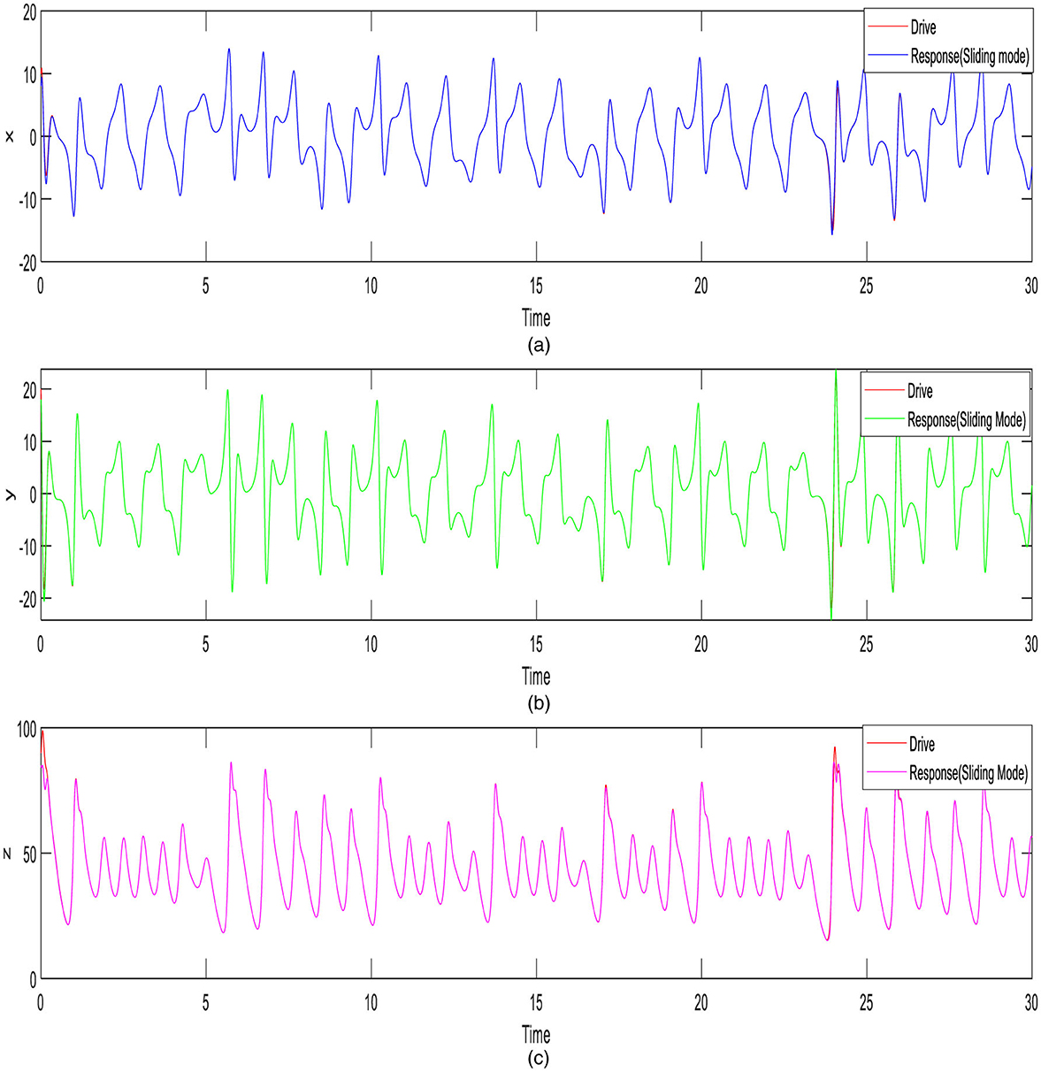
Figure 5. Interval retort of states for synchronization when the sliding mode controller is started t = 10: (a) x signs, (b) y signs, and (c) z signs.

Figure 6

Figure 6. Interval retort of states for synchronization when the sliding mode controller is started t = 5: (a) x signs, (b) y signs, and (c) z signs.

Figure 7

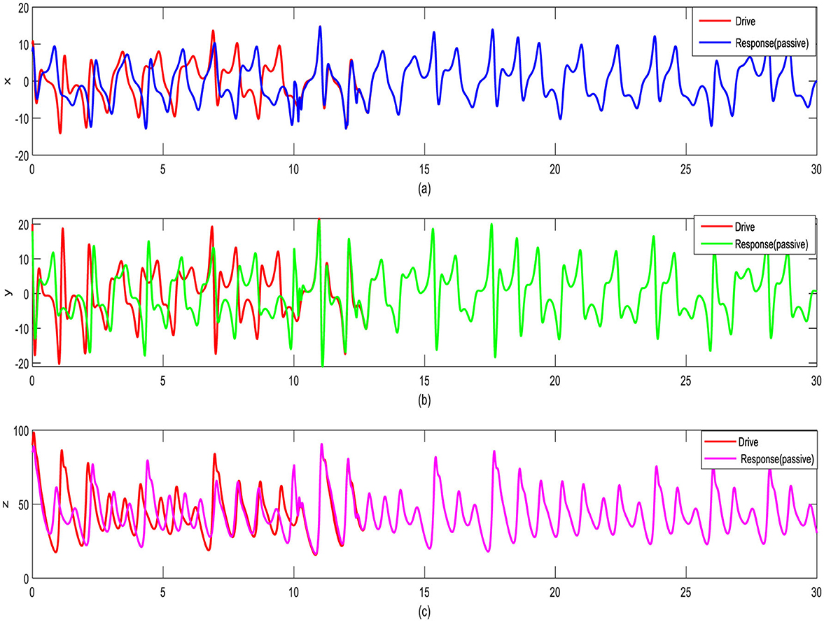
Figure 7. Interval retort of states for synchronization when the passive controller is started t = 10: (a) x signs, (b) y signs, and (c) z signs.

Figure 8

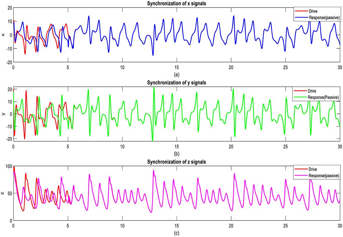
Figure 8. Interval retort of the states for synchronization when the passive controller is started t = 5: (a) x signs, (b) y signs, and (c) z signs.

Figure 9

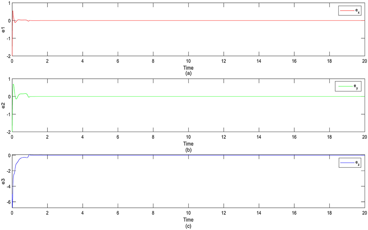
Figure 9. Retort of error signs for synchronization when the sliding mode controller is activated t = 10: (a) e₁ signs, (b) e₂ signs, and (c) e₃ signs.

Figure 10

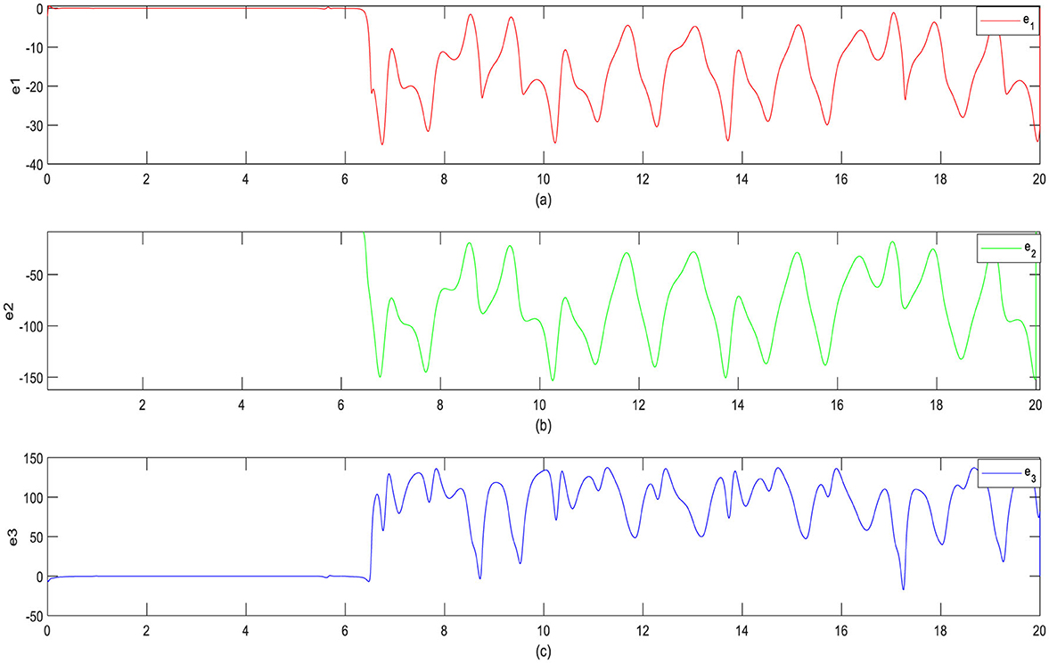
Figure 10. Retort of error signs for synchronization when the sliding mode controller is activated t = 5: (a) e₁ signs, (b) e₂ signs, and (c) e₃ signs.

Figure 11

Figure 11. Retort of error signs for synchronization when the passive controller is activated t = 10: (a) e₁ signs, (b) e₂ signs, and (c) e₃ signs.

Figure 12

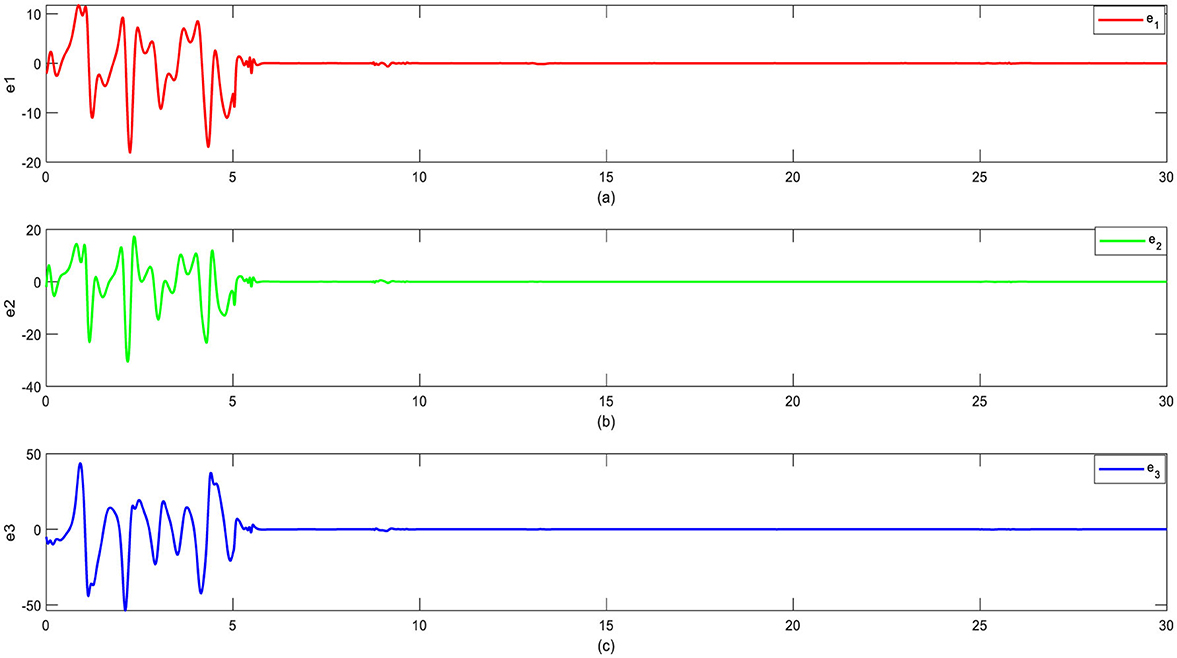
Figure 12. Retort of error signs for synchronization when the passive controller is started t = 5: (a) e₁ signs, (b) e₂ signs, and (c) e₃ signs.

Conclusion

The foremost empirical of this exploration is to investigate the synchronization of chaos in a non-linear finance system using the Liu dynamical system. A low-dimensional financial system can adjust to the global macroeconomic system through synchronization. Rapid fluctuations in factors such as price and interest rates are the primary causes of changes in demand and volume. Rapid changes in factors such as price and interest rates are the main drivers behind shifts in demand and volume. These cause non-linearity within a system. Alignment with the global financial system offers advantages for economic growth by achieving uniform interest rates, investment demand, and price levels. In addition, it can help mitigate uneven economic risks. Two sliding mode controllers and one passive controller have been created using the theories of sliding mode and passive control to bring two identical chaotic financial systems into synchrony. All theoretical analyses of the proposed methods of control successfully synchronize the two chaotic financial systems based on numerical simulations. In each case depicted in Figures 5–12, sliding mode controllers are more effective than passive controllers at controlling the synchronization of chaotic finance systems; thus, the sliding mode approach is more suitable. The benefit of the passive control approach is that it allows chaotic financial systems to be synchronized with a single controller, making implementation easier. The passive control merely modifies the interest rate, whereas the sliding mode control achieves synchronization by modifying both the interest rate and investment demand. The study helps researchers choose the best technique depending on system restrictions by highlighting the trade-offs between the two approaches.

Data availability statement

The original contributions presented in the study are included in the article/supplementary material, further inquiries can be directed to the corresponding author.

Author contributions

AA: Writing – original draft, Writing – review & editing. MA: Writing – review & editing. SA: Data curation, Formal analysis, Resources, Software, Writing – review & editing.

Funding

The author(s) declare that no financial support was received for the research and/or publication of this article.

Conflict of interest

The authors declare that the research was conducted in the absence of any commercial or financial relationships that could be construed as a potential conflict of interest.

Generative AI statement

The author(s) declare that no Gen AI was used in the creation of this manuscript.

Publisher's note

All claims expressed in this article are solely those of the authors and do not necessarily represent those of their affiliated organizations, or those of the publisher, the editors and the reviewers. Any product that may be evaluated in this article, or claim that may be made by its manufacturer, is not guaranteed or endorsed by the publisher.

References

1. Kocamaz UE, Goksu A, Taşkin H, Uyaroglu Y. Synchronization of chaos in nonlinear finance system by means of sliding mode and passive control methods: a comparative study. Inform Technol Cont. (2015) 44:7732. doi: 10.5755/j01.itc.44.2.7732

Crossref Full Text | Google Scholar

2. Cai GL, Yang MZ. Globally exponentially attractive set and synchronization of a novel three dimensional chaotic finance system. In: 2010 Third International Conference on Information and Computing. Wuxi: IEEE (2010).

Google Scholar

3. Ma JH, Chen YS. Study for the bifurcation topological structure and the global complicated character of a kind of nonlinear finance system(I). Appl Mathem Mechan. (2001) 22:1240–51. doi: 10.1007/BF02437847

Crossref Full Text | Google Scholar

4. Lorenz EN. Deterministic non-periodic flows. J Atmosph Sci. (1963) 20:130–41.

Google Scholar

5. Sparrow C. The Lorenz Equations: Bifurcation, Chaos and Strange Attractor. New York: Springer-Verlag (1982). p.269.

Google Scholar

6. Lü J, Chen G, Zhang S. The compound structure of a new chaotic attractor. Chaos Solitons Fract. (2002) 14:669–72. doi: 10.1016/S0960-0779(02)00007-3

Crossref Full Text | Google Scholar

7. Chen G, Ueta T. Yet another chaotic attractor. Int J Bifurcat Chaos. (1999) 9:1465–6. doi: 10.1142/S0218127499001024

Crossref Full Text | Google Scholar

8. Rössler OE. An Equation for continuous chaos. Phys Lett A. (1976) 57:397–8. doi: 10.1016/0375-9601(76)90101-8

Crossref Full Text | Google Scholar

9. Liu C, Liu T, Liu L, Liu K. A new chaotic attractor. Chaos Solitons Fract. (2004) 22:1031–8. doi: 10.1016/j.chaos.2004.02.060

Crossref Full Text | Google Scholar

10. Pukdeboon C. A review of fundamentals of Lyapunov theory. J Appl Sci. (2011) 10:2.

Google Scholar

11. Utkin VI. Variable structure systems with sliding mode. IEEE Trans Autom Cont. (1977) 22:212–22. doi: 10.1109/TAC.1977.1101446

Crossref Full Text | Google Scholar

12. Liu J, Wang X. Advanced Sliding Mode Control for Mechanical Systems: Design, Analysis, MATLAB Simulation. Cham: Springer. (2012).

Google Scholar

13. Bartoszewicz A, Żuk J. Sliding mode control — Basic concepts and current trends. In: IEEE International Symposium on Industrial Electronics. Bari: IEEE (2010).

Google Scholar

14. Wang FQ, Liu CX. Synchronization of hyperchaotic Lorenz system based on passive control. Chin Phys. (2006) 15:1971–5. doi: 10.1088/1009-1963/15/9/012

Crossref Full Text | Google Scholar

15. Idowu BA, Vaidyanathan S, Sambas A, Olusola OI, Onma OS. A New Chaotic Finance System: Its Analysis, Control, Synchronization and Circuit Design. Cham: Springer (2018).

Google Scholar

16. Strotz RH, McAnulty JC, Naines JB. Goodwin's nonlinear theory of the business cycle: an electro-analog solution. Econometrica. (1953) 21:390–411. doi: 10.2307/1905446

Crossref Full Text | Google Scholar

17. Yu H, Cai G, Li Y. Dynamic analysis and control of a new hyperchaotic finance system. Nonlin Dynam. (2012) 67:2171–82. doi: 10.1007/s11071-011-0137-9

Crossref Full Text | Google Scholar

18. De Cesare L, Sportelli M. A dynamic IS-LM model with delayed taxation revenues. Chaos Solitons Fract. (2005) 25:233–44. doi: 10.1016/j.chaos.2004.11.044

Crossref Full Text | Google Scholar

19. Chian ACL. Nonlinear dynamics and chaos in macroeconomics. Int J Theoret Appl Finance. (2000) 3:601. doi: 10.1142/S0219024900000723

Crossref Full Text | Google Scholar

20. Dousseh PY, Ainamon C, Miwadinou CH, Monwanou AV, Orou JB. Chaos in a Financial System With Fractional Order and Its Control via Sliding Mode. Hindawi: World Academic Press (2021).

Google Scholar

21. Liao Y, Zhou Y, Xu F, Shu XB. A study on the complexity of a new chaotic financial system, Complexity. (2020) 2020:8821156. doi: 10.1155/2020/8821156

Crossref Full Text | Google Scholar

22. Konishi K, Hirai M, Kokame H. Sliding mode control for a class of chaotic systems. Physics Letters A. (1998) 245:511–7. doi: 10.1016/S0375-9601(98)00439-3

Crossref Full Text | Google Scholar

23. Wu XJ, Liu JS, Chen GR. Chaos synchronization of Rikitake chaotic attractor using the passive control technique. Nonlinear Dynam. (2008) 53:45–53. doi: 10.1007/s11071-007-9294-2

Crossref Full Text | Google Scholar

24. Wang FQ, Liu CX. Synchronization of unified chaotic system based on passive control. Physica D. (2007) 225:55–60. doi: 10.1016/j.physd.2006.09.038

Crossref Full Text | Google Scholar

25. Sundarapandian V, Sivaperumal S. Global chaos synchronization of hyperchaotic Chen system by sliding mode control. Int J Eng Sci Technol. (2011) 3:4265–71.

Google Scholar

26. Cai GL, Yu HJ, Li YX. Stabilization of a modified chaotic finance system. In: Fourth Int. Conf. on Information and Computing, ICIC. Phuket: IEEE (2011). p. 188–191. doi: 10.1109/ICIC.2011.110

Crossref Full Text | Google Scholar

27. Emiroglu S, Uyaroglu Y, Koklukaya E. Control of a chaotic finance system with passive control. In: 3rd International Symposium on Sustainable Development. Sarajevo: IEEE (2012). p. 125–130.

Google Scholar

28. Uyaroglu Y, Temel R, Kirlioglu H. Feedback control of chaos in a hyperchaotic finance system. In: 3rd Int. Symp. on Sustainable Development. Sarajevo: IEEE (2012). p. 135–138.

Google Scholar

29. Yang M, Cai G. Chaos control of a non-linear finance system. J Uncert Syst. (2011) 5:263–70.

Google Scholar

30. Dadras S, Momeni HR. Control of a fractional order economical system via sliding mode. Physica A Stat. Mech. Appl. (2010) 389:2434–42. doi: 10.1016/j.physa.2010.02.025

Crossref Full Text | Google Scholar

31. Jabbari A, Kheiri H. Anti-synchronization of a modified three-dimensional chaotic finance system with uncertain parameters via adaptive control. Int J Nonlinear Sci. (2012) 14:178–85.

Google Scholar

32. Kareem SO, Ojo KS, Njah AN. Function projective synchronization of identical and non identical modified finance and Shimizu–Morioka systems. Pramana. (2012) 79:71–9. doi: 10.1007/s12043-012-0281-x

Crossref Full Text | Google Scholar

33. Li J, Xie CR. Synchronization of the modified financial chaotic system via a single controller. In: Int. Conf. on Frontiers of Manufacturing Science and Measuring Technology, ICFMM2011. Chongqing: Advanced Materials Research (2011). p. 1045–1048.

Google Scholar

34. Yu J, Vincent TL. Investigation on control of chaos. Chin J Aeronaut. (1997) 10:233–8.

Google Scholar

35. Lü JH, Lu NJ. Controlling Uncertain Lü system using linear feedback. Chaos, Solitons & Fractals. (2003) 17:127–33. doi: 10.1016/S0960-0779(02)00456-3

Crossref Full Text | Google Scholar

36. Gambino M, Lombardo G, Sammartino M. Global linear feedback control for the generalized lorenz system. Chaos Solitons Fractals. (2006) 29:829–37. doi: 10.1016/j.chaos.2005.08.072

Crossref Full Text | Google Scholar

37. Hegazi A, Agiza HN, El-Dessoky MM. Controlling chaotic behaviour for spin generator and rossler dynamical systems with feedback control. Chaos Solitons Fractals. (2001) 12:631–58. doi: 10.1016/S0960-0779(99)00192-7

Crossref Full Text | Google Scholar

38. Zhu C, Chen Z. Feedback control strategies for the Liu chaotic system. Physics Letters A. (2008) 372:4033–6. doi: 10.1016/j.physleta.2008.03.018

Crossref Full Text | Google Scholar

39. Matouk AE. Dynamical analysis, feedback control and synchronization of Liu dynamical system. Nonlinear Analy. (2008) 69:3213–24. doi: 10.1016/j.na.2007.09.029

PubMed Abstract | Crossref Full Text | Google Scholar

40. Jiang J, Cao D, Chen H. Sliding mode control for a class of variable -order fractional chaotic systems. J Franklin Instit. (2020) 357:10127–58. doi: 10.1016/j.jfranklin.2019.11.036

PubMed Abstract | Crossref Full Text | Google Scholar

41. Shokouhi F, Markazi D, Hossein A. A new continuous approximation of sign function for sliding mode control. In: International Conference on Robotics and Mechantronics. Tehran: Iran University of Science and Technology (2018).

Google Scholar

42. Vaidyanathan S, Sampath S. Global chaos synchronization of hyperchaotic Lorenz system by sliding mode control. Int J Eng Sci Technol. (2011) 3:4265–71. doi: 10.1007/978-3-642-24055-3_16

Crossref Full Text | Google Scholar

43. Jiao ZQ, An LJ. Passive control and synchronization of hyperchaotic Chen system. Chinese Phys. B (2008) 17:492. doi: 10.1088/1674-1056/17/2/025

Crossref Full Text | Google Scholar