Assessing the role of model choice in parameter identifiability of cancer treatment efficacy

Several mathematical models are commonly used to describe cancer growth dynamics. Fitting of these models to experimental data has not yet determined which particular model best describes cancer growth. Unfortunately, choice of cancer growth model is known to drastically alter the predictions of both future tumor growth and the effectiveness of applied treatment. Since there is growing interest in using mathematical models to help predict the effectiveness of chemotherapy, we need to determine if the choice of cancer growth model affects estimates of chemotherapy efficacy. Here, we simulate an in vitro study by creating synthetic treatment data using each of seven commonly used cancer growth models and fit the data sets using the other (“wrong”) cancer growth models. We estimate both the ε_max (the maximum efficacy of the drug) and the IC₅₀ (the drug concentration at which half the maximum effect is achieved) in an effort to determine whether the use of an incorrect growth model changes the estimates of chemotherapy efficacy parameters. We find that IC₅₀ is largely weakly practically identifiable no matter which growth model is used to generate or fit the data. The ε_max is more likely to be practically identifiable, but is sensitive to choice of growth model, showing poor identifiability when the Bertalanffy model is used to either generate or fit the data.

1 Introduction

Cancer is a leading cause of death and causes a serious burden for patients and society even when it isn't fatal [1]. While new cancer treatment modalities are constantly being developed [2–4], chemotherapy is still one of the primary treatments for cancer. However, even chemotherapy is constantly being improved with the development of new drugs [5, 6] and new drug delivery methods [7, 8] that, hopefully, reduce side effects while maintaining drug effectiveness.

New chemotherapeutics and new drug delivery systems need to be tested in vitro before they can be considered for use in humans. The standard method for characterizing chemotherapy is to generate a dose-response curve by measuring the amount of cancer cell death at a particular time as a function of the drug dose [9]. The resulting curve is characterized by two parameters: the maximum effect of the drug (ε_max), and the drug effect at which we achieve half the maximum effect (IC₅₀). While both quantities are needed to fully characterize the effectiveness of a drug, often only the IC₅₀ is reported. It has also been noted that the dose response curve, and therefore the estimates of IC₅₀ and ε_max, depend on the time at which the cell death measurement is made [10–13]. This can lead to incorrect dosing when moving to animal and human studies [14–18] and might lead to the conclusion that the drug is ineffective or too toxic. For this reason, new methods for quantifying the effectiveness of a drug have been proposed and are being tested [11–13, 19–21].

One suggestion is to use tumor growth time courses, both control and treated, along with a mathematical model of cancer growth to extract estimates of the IC₅₀ and ε_max assuming that the drug alters the growth rate of the tumor [20, 21]. The experimental protocol for this can be implemented using either traditional wells [21] or spherical organoids [22–24]. While this method yields IC₅₀ and ε_max estimates that do not depend on a particular measurement time, there are potential drawbacks to using this method. One major concern is that there are several different mathematical models that are used to describe cancer growth [25–27]. Comparison of the models shows that they can lead to very different predicted outcomes when used to simulate tumors [25, 28]. Other studies have found that using different tumor growth models can lead to different predictions of treatment effectiveness [18, 20, 29]. Researchers have tried to determine which of these models best describes cancer growth [30–35] with results suggesting that the best model depends on the details of the experiment [32, 33]. Since it is not clear which growth model most accurately represents the growth of the cancer cells used in a particular drug characterization experiment, we need to determine whether the drug effectiveness parameters depend on the choice of growth model.

The issue of how model structure affects the predictions made by models is an issue encountered in many fields [36–40]. Note that this is a slightly different question than how uncertainty in experimental data affects model predictions and parameter estimates which has been widely studied [41–43]. How erroneous model structure affects parameter estimation is less frequently addressed, although there have been some attempts to understand how using incorrect model structure affects parameter estimation [36, 44–46]. Some studies have examined the relative contribution of model structure uncertainty to uncertainty in parameter estimates and in resulting model predictions [47, 48], although it is unclear whether the methods used to determine these estimates are generalizable to other models and systems. Suggestions have also been made on how to potentially deal with model structure uncertainty, including the use of hybrid models that incorporate measured data [49–51] or machine learning [52], but this is not always feasible.

In this paper, we study the effect of growth model choice on estimates of drug effectiveness parameters. We use seven common ODE cancer growth models to generate data that is then fit by the other models. We find that most of the models are interchangeable and lead to similar estimates of IC₅₀ and ε_max, with the exception of the Bertalanffy model, which leads to incorrect estimates of ε_max. We also find, however, that using this method to estimate other, non-drug-related, parameters of the growth models can lead to inaccurate estimates of these parameters.

2 Materials and methods

2.1 Generating tumor growth time courses

We used the seven commonly used cancer growth ordinary differential equation models [25] shown in Table 1. Brief explanations of each model are given below:

• Exponential: in the early stages of tumor growth, cells divide regularly, creating two daughter cells each time. A natural description of the early stages of cancer growth is thus the exponential model [53], where growth is proportional to the population. This model predicts early growth very well, but is known to fail at later stages when angiogenesis and nutrient depletion begin to play a role [26, 33].

• Mendelsohn: the Mendelsohn model is a generalization of the exponential growth model where growth is proportional to some power of the current population [54]. This can help account for different spatial geometries of cancer growth.

• Logistic: the logistic (or Pearl-Verhulst) equation was created by Pierre Francois Verhulst in 1838 [55]. This model describes the growth of a population that is limited by a carrying capacity. The logistic equation assumes that the growth rate decreases linearly with size until it equals zero at the carrying capacity.

• Linear: we use a slightly modified version of a linear growth model. This version assumes initial exponential growth that changes to growth that is constant over time. A linear growth model was used in early research to analyze growth of cancer cell colonies [56].

• Surface: the surface model assumes only a thin layer of cells at the surface of the tumor are dividing while the cells inside the solid tumors do not reproduce [57]. Our formulation again assumes exponential growth at early times with the surface growth taking over at longer times.

• Bertalanffy: the Bertalanffy equation was created by Ludwig Bertalanffy as a model for organism growth [58]. This model assumes that growth occurs proportional to surface area, but that there is also a decrease of tumor volume due to cell death. This model was shown to provide the best description of human tumor growth [31].

• Gompertz: Benjamin Gompertz originally created the Gompertz model in 1825 in order to explain human mortality curves [59]. The model is a generalization of the logistic model with a sigmoidal curve that is asymmetrical with the point of inflection. The curve was eventually applied to model growth in size of entire organisms [60] and more recently, was shown to provide the best fits for breast and lung cancer growth [33].

Table 1

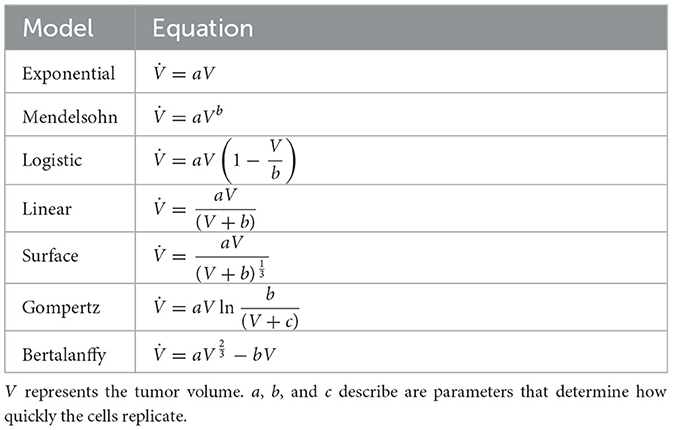
Table 1. ODE tumor growth models.

Model parameters were taken from fits to experimental data [25] and are given in Table 2. These parameters are such that all models had essentially the same time course over the first 60 days of the tumor. Each of these models was used to generate several synthetic data sets consisting of a control tumor time course and five treated tumor time courses, each at a different concentration of drug.

Table 2

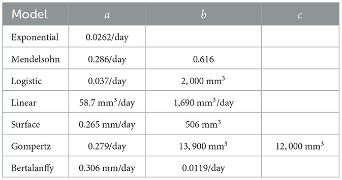
Table 2. Model parameters.

Chemotherapy is assumed to affect the growth rate of each model and is modeled using the E_max model [61],

$\epsilon =\frac{{\epsilon }_{\max }D}{{\text{IC}}_{50}+D},$

where ε is the efficacy of the drug, ε_max is the maximum efficacy of the drug, IC₅₀ is the drug dose at which half the maximum effect is achieved, and D is the dose of the drug. Growth rate is modified by multiplying the parameter a in each model by (1−ε). We assume an ε_max value of 1 and an IC₅₀ of 1, which simply means that we are measuring the drug dose relative to the IC₅₀. Drug dose is assumed to be constant over the entire course of the experiment. Tumor time courses are simulated for 14 days, with tumor volume measurements taken every 2 days (see Figure 1, top left). We then added Gaussian noise to each data point at levels of 5%, 10%, and 20%. This was done by drawing a random number from the distribution

$\begin{array}{ll}f(x)=\frac{1}{\sqrt{2\pi {\sigma }^2}}{e}^{-\frac{x^2}{2{\sigma }^2}},& (1)\end{array}$

where we have assumed a mean value of 0, and σ is 5%, 10%, or 20% of the value of the data point. This number is then added to the original data point. 10 synthetic data sets were generated for each model at each of the three noise levels. Example data sets for the exponential model are shown in Figure 1.

Figure 1

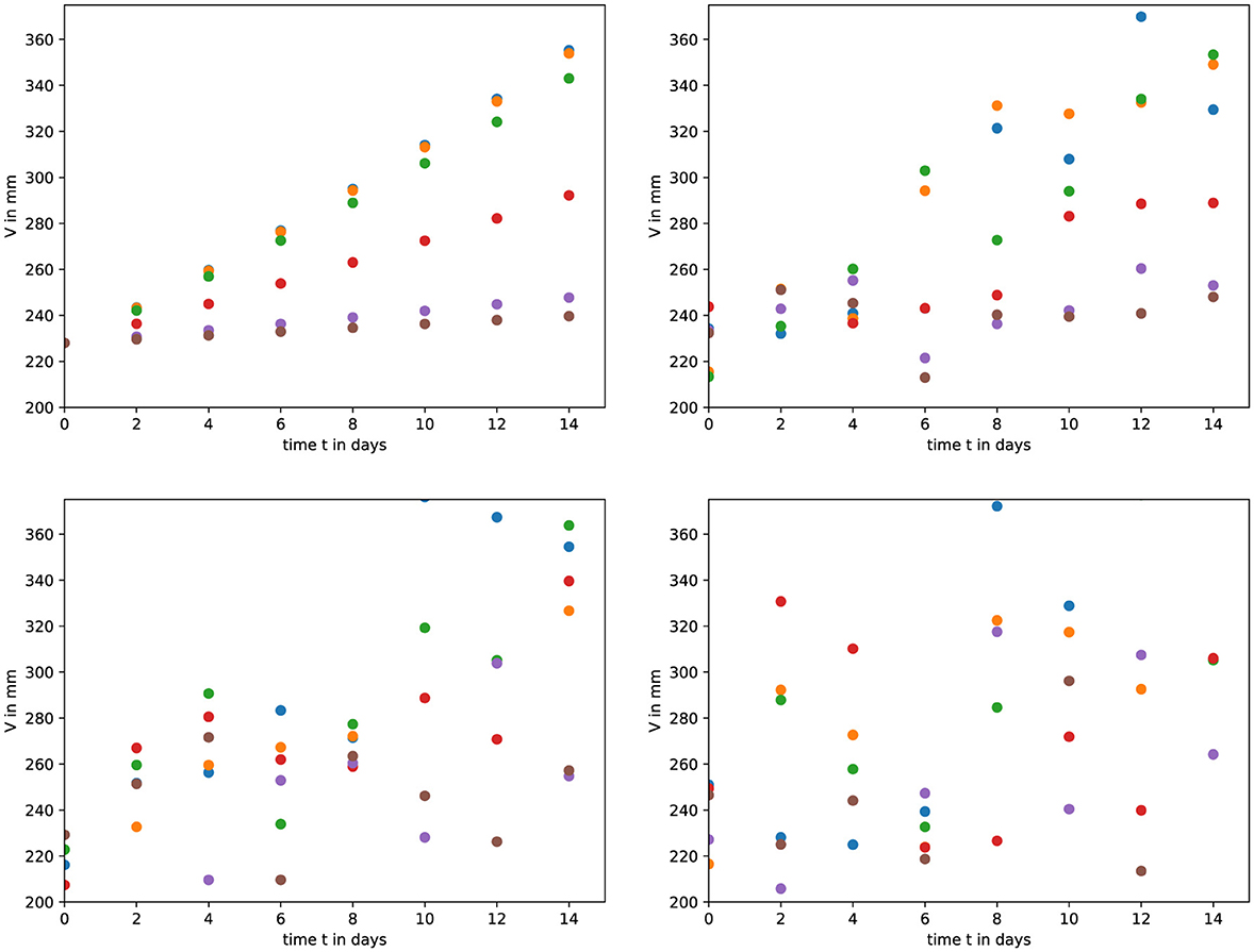
Figure 1. An example of the synthetic data. (top left) We used the exponential model to generate a control and five treated tumor time courses. We then added Gaussian noise of (top right) 5%, (bottom left) 10%, and (bottom right) 20%.

2.2 Fitting models to data

In order to test whether drug effectiveness measurements are robust to incorrect model choice, each of the synthetic data sets was fit using each of the growth models to extract estimates for model parameters and for ε_max and IC₅₀. Fitting was done using Python's scipy.minimize function using the Nelder-Mead algorithm to minimize the sum of squared residuals,

$\text{SSR}={\displaystyle \sum }{(y_{\text{data}}-y_{\text{fit}})}^2,$

where y_data is the synthetic data, and y_fit is the model's predicted tumor volume. Bounds were used to limit the parameter space when fitting and are given in Table 3. We used the base model parameters as the initial guess when fitting. Note that while cancer growth is exponential, our time courses are over a short time period and the variation in tumor volume is less than an order of magnitude. Parameter estimates retrieved from the model fits for the 10 synthetic data sets for each of the seven models at each noise level were compared to the expected values of the parameters. Sample code for both generating and fitting the models is available at https://github.com/hdobrovo/Efficacy_robustness.

Table 3

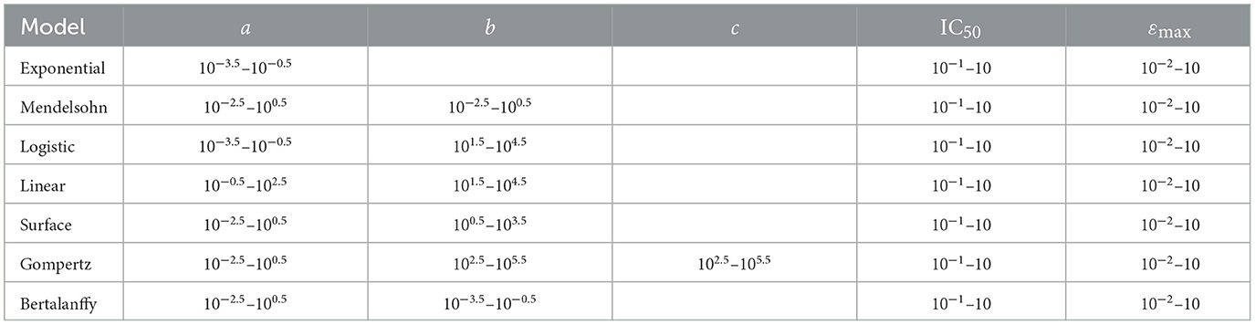
Table 3. Bounds used for model fitting.

We use the average relative error,

$\begin{array}{ll}\text{ARE}=100\%\times \frac{1}{N}{\displaystyle \sum _{i=1}^N}\frac{|{\theta }_0-{\theta }_i|}{\left|{\theta }_0\right|},& (2)\end{array}$

where θ₀ is the known parameter value, and θ_i is the estimated parameter value. The ARE is used to judge practical identifiability of parameters with rough guidelines as follows: if ARE(θ) < σ, where sigma is the amount of added noise, the parameter is considered identifiable; if σ < ARE(θ) < 10σ, the parameter is considered weakly identifiable; and if 10σ < ARE(θ), the parameter is not identifiable [38].

3 Results

3.1 Estimating drug efficacy parameters

Since the primary motivation for this work is to determine whether drug effectiveness parameter estimates are robust to the choice of growth model, we first examine whether the growth models were able to return the correct values of IC₅₀ and ε_max. Figure 2 shows the estimated values of IC₅₀ for synthetic data sets generated with different cancer growth models. The title of each plot indicates the model used to generate the synthetic data, while the models used to fit the data are listed along the x-axis. The expected value of IC₅₀ (IC₅₀ =1) is indicated by the solid red line. The colored bars indicate the interquartile range of the estimates with the error bars extending to the 95% confidence intervals, estimated from the fitted parameter values. Stars indicate outlier estimates. We also include the ARE values for IC₅₀ in Table 4. The columns indicate which model was used to fit the data, while the horizontal headings indicate the model used to generate the data. ARE values suggesting practical identifiability are given in bold and those suggesting weak practical identifiability are given in italics.

Figure 2

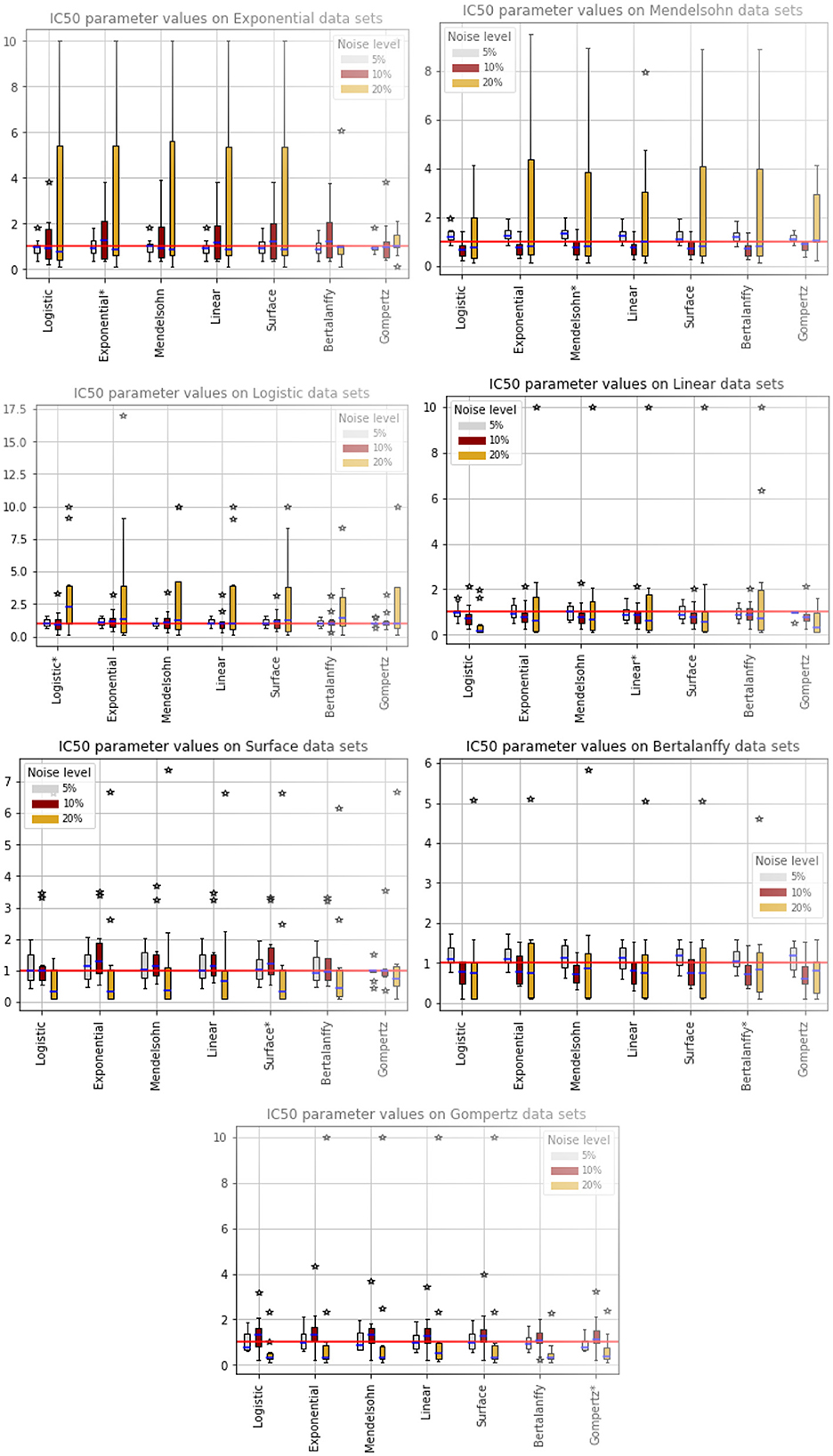
Figure 2. Estimated values of IC₅₀. The title indicates the model used to generate the synthetic data, while the models along the x-axis indicate the model used to fit the data. The solid red line indicates the expected value of IC₅₀. The colored bars indicate the interquartile range of the estimates with the error bars extending to the 95% confidence intervals. Stars indicate outlier estimates.

Table 4

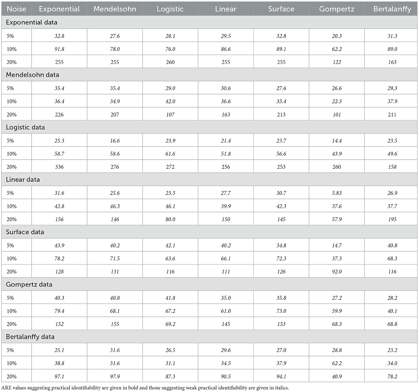
Table 4. ARE values for IC₅₀ for the different models.

Data generated by the exponential model (Figure 2, top left) and fit by other models returns IC₅₀ values close to the expected value when there is 5% or 10% noise. With 20% noise, most of the models return IC₅₀ estimates that are larger than the expected value. The two exceptions are the Bertalanffy model, which slightly underestimates the IC₅₀ and the Gompertz, which slightly overestimates the IC₅₀. While the IC₅₀ values are close to the expected value, ARE indicates that IC₅₀ is weakly practically identifiable in almost all cases. Data generated by the Mendelssohn model (Figure 2, top right) leads to fits that tend to slightly overestimate IC₅₀ at 5% noise, underestimate IC₅₀ at 10% noise, and return large values of IC₅₀ at 20% noise. All models return correct estimates of IC₅₀ when fit to data generated by the logistic model (Figure 2, second row left) with 5% noise. The models start to overestimate the IC₅₀ with 10% noise and with 20% noise, the models are returning fairly large estimates of IC₅₀. Data generated with the linear model (Figure 2, second row right) leads to fairly accurate estimates of IC₅₀ when there is 5% noise, tends to underestimate IC₅₀ when there is 10% noise, and even returns somewhat accurate IC₅₀ estimates at 20% noise except for the occasional outlier. The data generated by the surface model (Figure 2, third row left) shows slightly more error in IC₅₀ estimates at the 5% noise level than does data generated by other models. However, the error in IC₅₀ at the 20% noise level is smaller than for data generated by other models, although we observe some large outlier estimates again. Data generated by the Bertalanffy model (Figure 2, third row right) also leads to IC₅₀ estimates with small amounts of error, even at the 20% noise level, although the IC₅₀ is generally underestimated at the 10% and 20% noise levels. Finally, data generated by the Gompertz model (Figure 2, bottom) leads to fairly consistent estimates of IC₅₀, although there are some large outlier estimates when there is a large amount of noise.

While IC₅₀ is the quantity most often used to characterize the effectiveness of chemotherapy, ε_max is also needed to fully describe a dose-response curve. We show the estimated values of ε_max in Figure 3, where again the model used to generate the data is indicated in the title, while the model used to fit the data is indicated along the x-axis. The expected value of ε_max is indicated by the solid red line and stars indicate outlier estimates. We also include the ARE values for ε_max in Table 5. The columns indicate which model was used to fit the data, while the horizontal headings indicate the model used to generate the data. ARE values suggesting practical identifiability are given in bold and those suggesting weak practical identifiability are given in italics.

Figure 3

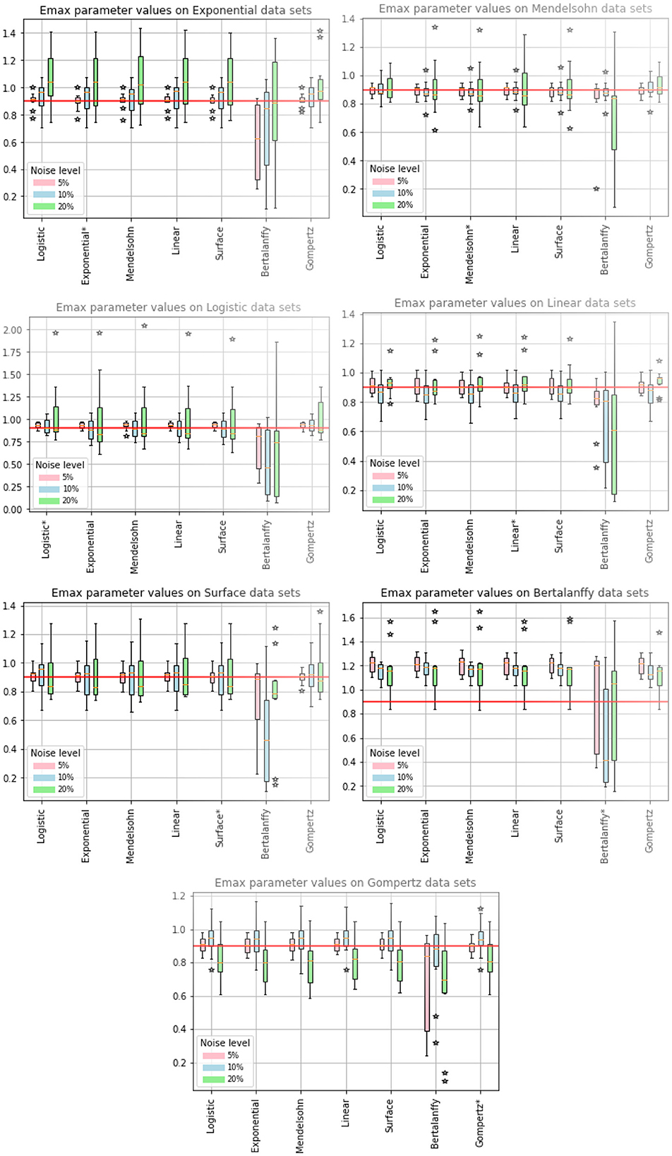
Figure 3. Estimated values of ε_max. The title indicates the model used to generate the synthetic data, while the models along the x-axis indicate the model used to fit the data. The solid red line indicates the expected value of ε_max. The colored bars indicate the interquartile range of the estimates with the error bars extending to the 95% confidence intervals. Stars indicate outlier estimates.

Table 5

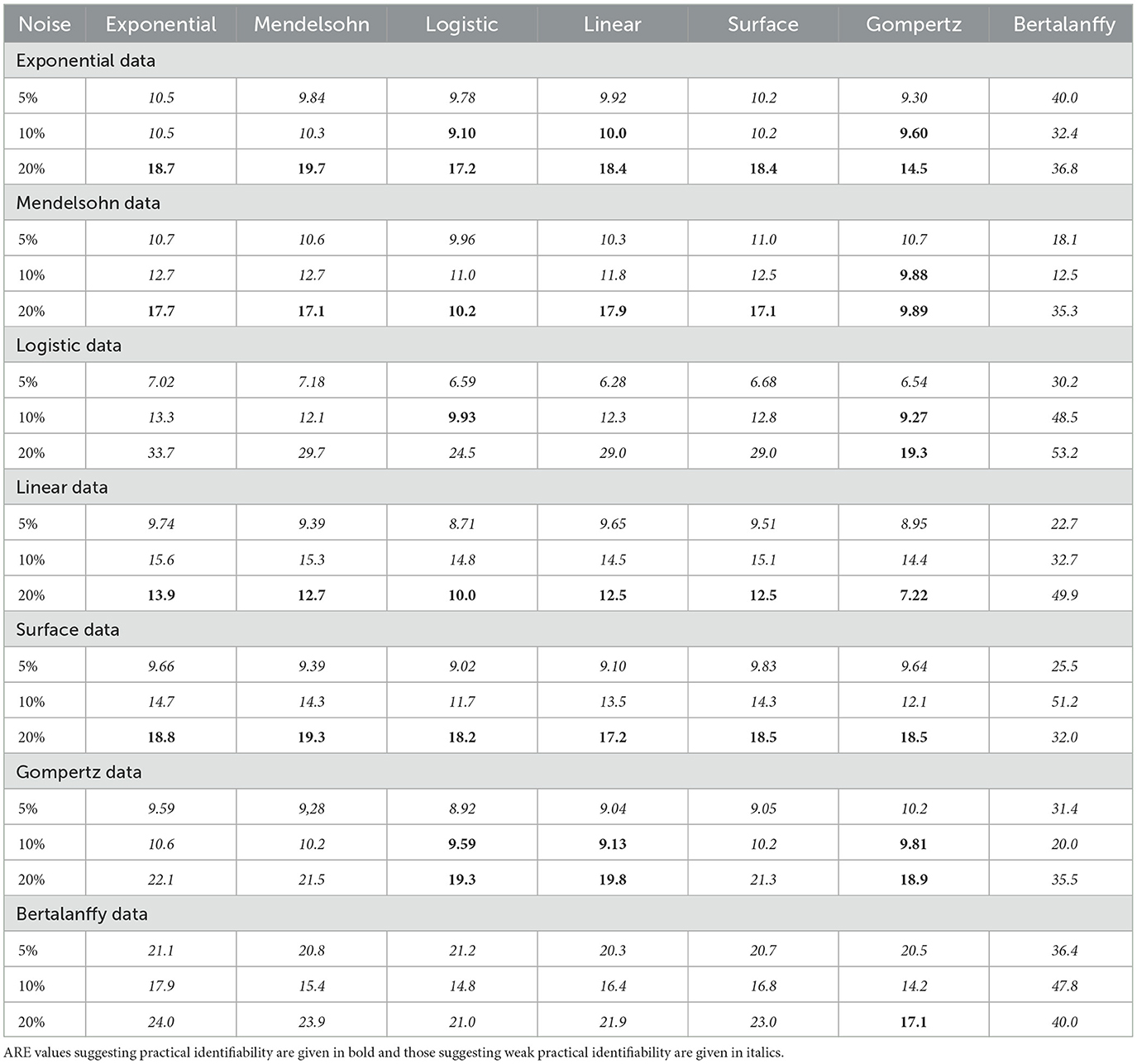
Table 5. ARE values for ε_max for the different models.

We first note that when the Bertalanffy model is used to fit data, no matter which model was used to generate the data, the estimated values of ε_max tend to be different from the estimates generated by fits using the other models, which also results in higher values of ARE. When the Bertalanffy model is used to generate the data, using other models to fit the data leads to overestimation of ε_max. This is quite different from what we observe for estimated values of IC₅₀, where no particular model seemed to stand out either when it was used to generate data or when it was used to fit data. The other model that stands out somewhat is the Gompertz model. When the Gompertz model is used to generate the data, the remaining models tend to underestimate the correct value of ε_max at high levels of noise. The remaining models return similar results when used for generating data and for fitting to return the ε_max estimates. ARE values for ε_max are notably lower than for IC₅₀, with many parameters being practically identifiable at least in some cases.

3.2 Estimating base model parameters

When fitting models to data, we also fit the model parameters (a, b, and c) along with the drug efficacy parameters IC₅₀ and ε_max. Thus we also checked whether our fits returned the correct values for these model parameters. Recall that the parameter values we used produce nearly identical untreated tumor growth curves regardless of which model is used to generate the data. The expectation then is that we will retrieve our original parameter values when we fit the data using a particular model, even when that model was not used to generate the data. Figures 4, 5 show the fitted parameter estimates when different models were used to generate the underlying data. Note that in these figures, the title indicates the model that was used to fit the data while the model used to generate the data is indicated along the x-axis. Figure 4 shows the results for the a parameter of each model and Figure 5 shows the results for the b (and c for the Gompertz model) parameters. We also include the ARE values for a in Table 6 and for b and c in Table 7. The columns indicate which model was used to generate the data, while the horizontal headings indicate the model used to fit the data. ARE values suggesting practical identifiability are given in bold and those suggesting weak practical identifiability are given in italics.

Figure 4

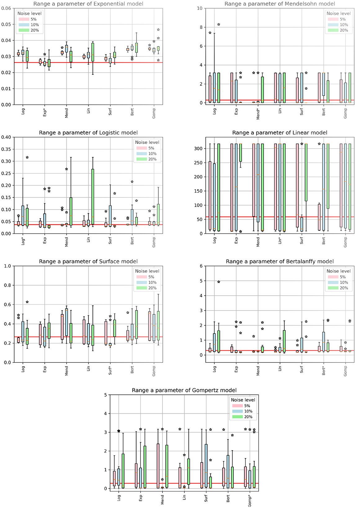
Figure 4. Estimated values of model parameters. The x-axis indicates the model used to generate the synthetic data, while the titles indicate the model used to fit the data. The solid red line indicates the expected value of the parameter. The colored bars indicate the interquartile range of the estimates with the error bars extending to the 95% confidence intervals. Stars indicate outlier estimates.

Figure 5

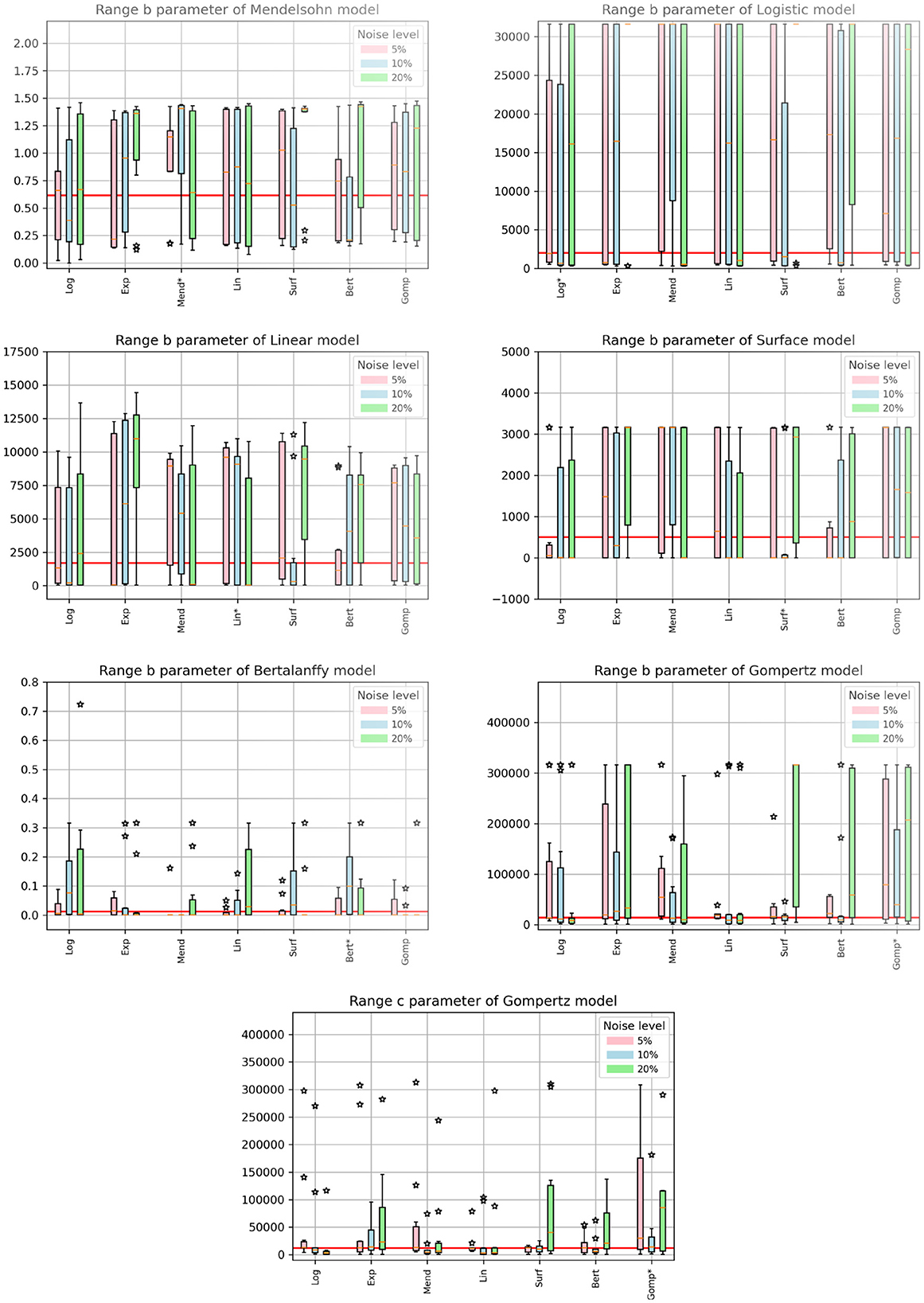
Figure 5. Estimated values of model parameters. The x-axis indicates the model used to generate the synthetic data, while the titles indicate the model used to fit the data. The solid red line indicates the expected value of the parameter. The colored bars indicate the interquartile range of the estimates with the error bars extending to the 95% confidence intervals. Stars indicate outlier estimates.

Table 6

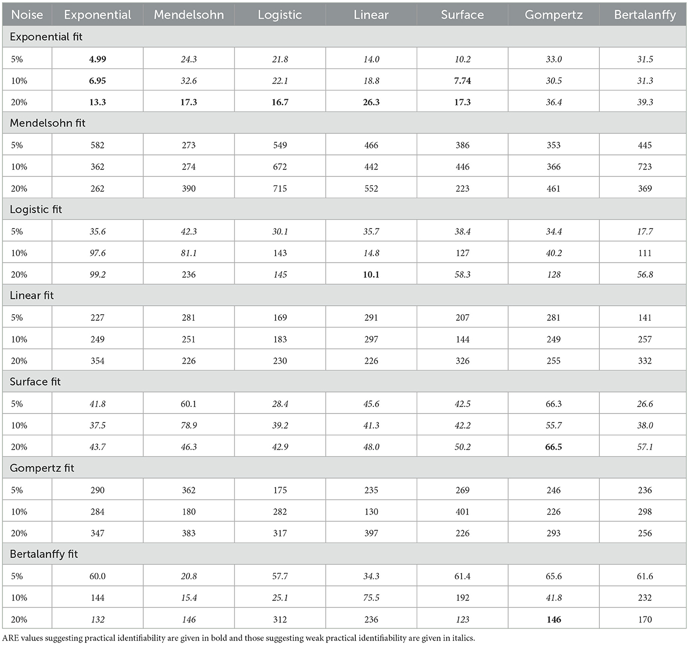
Table 6. ARE values for a parameter for the different models.

Table 7

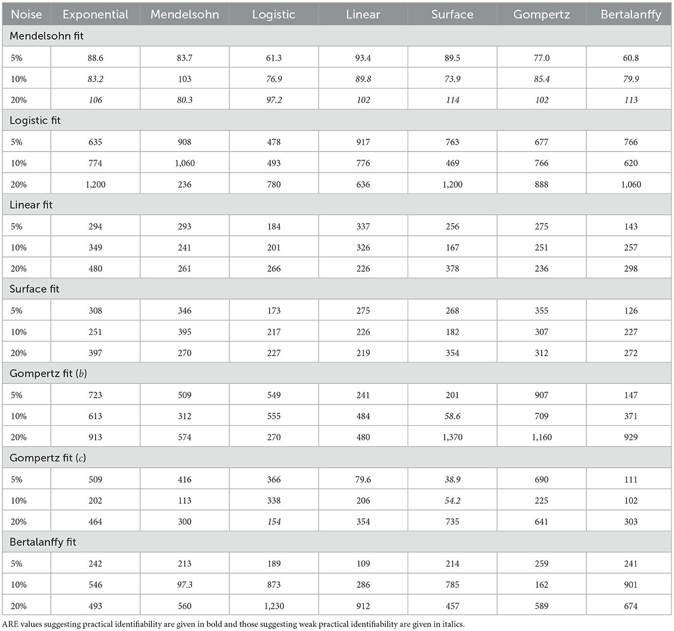
Table 7. ARE values for b and c parameters for the different models.

Interestingly, even when the same model is used to both generate the data and subsequently fit the data, we do not always get the correct parameter values. For example, the Mendelssohn model tends to underestimate its own a parameter, but overestimate its own b parameter, particularly at the 5% and 10% noise levels. The Gompertz model also tends to overestimate its own b and c values. ARE values suggest that many of these parameters are not identifiable, particularly the b and c parameters.

Some parameters appear to be more easily identifiable and robust to model choice, as indicated by the small error bars. Examples of these are the a parameters of the exponential, surface, and Bertalanffy models, as well as the b parameter of the Mendelssohn model. The ARE values for these parameters are also more likely to be at least weakly practically identifiable than other model parameters. Other parameters are difficult to identify with any sort of accuracy. Examples of these are the a parameter of the linear model and the b parameters of the logistic, linear, surface, and Bertalanffy models. The large error in the estimates of the b parameter of so many models might be due to the short duration of the data set. The b parameters in many of the models are determined by behavior at long time scales. For example, b is the carrying capacity of the logistic model and sets the maximum tumor size. Since the data set is not approaching the maximum size, there isn't sufficient information to determine these parameters accurately.

Perhaps one of the most interesting results is for the exponential model. Since the data is only taken over 14 days, a relatively short time frame even compared to the time constant for the exponential model (about 38 days), growth of the tumor should be well approximated by an exponential model. However, when using the exponential model to fit data generated by other functions, we find that we over-estimate the true growth rate (Figure 4, top left). A similar issue is observed with the estimated values of the a parameter of the logistic model, another commonly-used model for tumor growth. The a parameter for the logistic model also represents the exponential growth rate since the tumor sizes here are small compared to the carrying capacity. For the logistic model, the true value is usually within the 95% CI, but most estimates are higher than the true value.

4 Discussion

We used synthetic data generated with seven different cancer growth models to assess the robustness of estimates of IC₅₀ and ε_max to the incorrect choice of growth model. We found that IC₅₀ estimates were fairly robust to the choice of growth model, with accuracy of the estimate being determined more by the amount of added noise than by choice of growth model. ε_max, however, did show some dependence on the choice of growth model. In particular, when the Bertalanffy model was used to fit synthetic data generated by other models, it generally underestimated the correct value of ε_max. When the synthetic data was generated by the Bertalanffy model, the other models overestimated the correct value of ε_max. Note, however, that while we get consistent parameter estimates with most of the growth models, the parameters are mostly only weakly identifiable with these measurements.

It is not clear why the Bertalanffy model is an outlier in this study. The Bertalanffy model is able to fit cancer growth curves about as well as the other models [25, 33–35, 62, 63]. although it sometimes gives outlier predictions when chemotherapy is incorporated into the model [10, 28]. A possible reason for this is the mathematical formulation of the model (see Table 1). The Bertalanffy model assumes that there is a necrotic core whose size grows along with the tumor. The growth rate of the necrotic core is determined by the parameter b. When we apply the chemotherapy in our model, it is applied solely to the parameter a, so the growth of living tumor cells is slowed, but the growth of the necrotic core is not. This is different from all the other models where applying the drug to the parameter a reduces growth of the entire tumor since the other models do not include the assumption of some non-replicating cells. In this way, the volume predicted by the Bertalanffy model might actually shrink faster than other models (the term bV is negative and reduces the volume) than the volume predicted by other models, making it hard for the other models to correctly replicate this dynamic.

We also examined whether the untreated model parameter values (a, b, and c) were robust to model choice. We found that a mismatch between the generating model and the fitting model often leads to incorrect parameter estimates. In particular, the two most commonly used models, the exponential and logistic models [33, 62], overestimate the tumor growth rate when other models are used to generate the data. In reality, tumor growth is complex and most likely does not strictly follow either of these models, so when using exponential or logistic models to fit this data, researchers might be overestimating the growth rate. If modeling is being used to help personalize treatment for patients [64–67], this overestimation could have serious implications. A higher growth rate requires higher doses of chemotherapy, which could cause worse side effects for patients [68]. Some of the estimation error could be due to the type of data set used here. The data used for fitting included not only untreated tumor growth curves, but also treated tumor growth curves where the treatment was assumed to affect the growth rate. It's possible that using only the untreated growth curve will yield more accurate growth rate estimates.

We also found that several of the model parameter values were not really identifiable, as indicated by the large 95% confidence intervals. These tended to be parameter values that played a role in determining tumor growth over long time frames. This is not particularly surprising since our data sets were taken over a fairly short period of time. Such short duration data sets are not uncommon in cancer studies for a variety of reasons. In vitro studies often do not provide data for more than two weeks since cells tend to die after that time [21]. Small animal models also often cannot support tumor growth for longer than two or three weeks. This suggests that many available pre-clinical data sets are not long enough to accurately identify some of these parameters. For the purposes of using mathematical modeling to personalize treatment plans, often the untreated tumor growth curve is over a short time period [18, 65], and this is used to make predictions on possible treatment plans. This short time span could potentially lead to inaccurate parameter estimates that result in poor prediction of long-term treatment outcomes. These inaccuracies could be amplified by some of the issues faced in trying to translate parameter and/or growth model results from in vitro studies to in vivo animal studies and then to humans [14–18].

In addition to the short time span of the collected data, there are a number of simplifying assumptions made here that complicate parameter identifiability for in vivo systems. While maintaining a constant drug dose is possible for in vitro studies, modeling of in vivo studies will need to consider the pharmacokinetics of the drug [69, 70]. One study examined whether it was possible to model a time-varying drug concentration with a constant drug dose [71], finding that this was a reasonable assumption particularly at smaller doses. While that study examined treatment of a viral infection, it is likely also a reasonable assumption for treatment of cancer, particularly because cancer growth is typically on a slower time scale than the oscillations of the drug. An additional difficulty is that chemotherapy often has a number of effects on the tumor and it is not clear that modeling the effect of the drug as solely acting on the growth rate is a correct assumption [20, 72]. Further complicating the measurements done in vivo is the fact that tumors are heterogeneous and the cells contained within the tumor can respond differently to the drug [73]. There are also measurement factors for in vivo systems that impact parameter identifiability [74–77]. For example, there is often censored data — measurements below a certain threshold that cannot be accurately measured — that is discarded when fitting, which has been shown to affect parameter estimates [74]. The frequency of measurements [77] and the amount of noise in the measurements [77] also have a significant impact on our ability to identify model parameters. Finally, using proxy data, such as measurements of prostate-specific antigen, rather than direct measurements of the tumor volume also hampers our ability to properly identify model parameters [76].

5 Conclusion

This study has determined that using short time courses of tumor growth curves treated with different amounts of drug to estimate drug efficacy parameters leads to consistent estimates of IC₅₀ and ε_max for most tumor growth models, although they are mostly weakly practically identifiable. Estimation of the other model parameters using this data is generally not very accurate and could lead to overestimation of the growth rate and poor predictions of long-term behavior.

Data availability statement

The original contributions presented in the study are included in the article/Supplementary material, further inquiries can be directed to the corresponding author.

Author contributions

NK: Conceptualization, Data curation, Formal analysis, Investigation, Methodology, Software, Validation, Visualization, Writing – original draft. HD: Conceptualization, Methodology, Project administration, Supervision, Writing – review & editing.

Funding

The author(s) declare that financial support was received for the research and/or publication of this article. This research was supported by DAAD RISE.

Conflict of interest

The authors declare that the research was conducted in the absence of any commercial or financial relationships that could be construed as a potential conflict of interest.

The author(s) declared that they were an editorial board member of Frontiers, at the time of submission. This had no impact on the peer review process and the final decision.

Generative AI statement

The author(s) declare that no Gen AI was used in the creation of this manuscript.

Publisher's note

All claims expressed in this article are solely those of the authors and do not necessarily represent those of their affiliated organizations, or those of the publisher, the editors and the reviewers. Any product that may be evaluated in this article, or claim that may be made by its manufacturer, is not guaranteed or endorsed by the publisher.

Supplementary material

The Supplementary Material for this article can be found online at: https://www.frontiersin.org/articles/10.3389/fams.2025.1542617/full#supplementary-material

References

1. Smith GL, Lopez-Olivo MA, Advani PG, Ning MS, Geng Y, Giordano SH, et al. Financial burdens of cancer treatment: a systematic review of risk factors and outcomes. J Natl Compr Cancer Netw. (2019) 17:1184. doi: 10.6004/jnccn.2019.7305

PubMed Abstract | Crossref Full Text | Google Scholar

2. Gonzalez-Valdivieso J, Girotti A, Schneider J, Arias FJ. Advanced nanomedicine and cancer: challenges and opportunities in clinical translation. Intl J Pharmaceut. (2021) 599:120438. doi: 10.1016/j.ijpharm.2021.120438

PubMed Abstract | Crossref Full Text | Google Scholar

3. Zhan T, Rindtorff N, Betge J, Ebert MP, Boutros M. CRISPR/Cas9 for cancer research and therapy. Sem Cancer Biol. (2019) 55:106–19. doi: 10.1016/j.semcancer.2018.04.001

PubMed Abstract | Crossref Full Text | Google Scholar

4. Esfahani K, Roudaia L, Buhlaiga N, Del Rincon S, Papneja N, Miller W. A review of cancer immunotherapy: from the past, to the present, to the future. Curr Oncol. (2020) 27:S87–97. doi: 10.3747/co.27.5223

PubMed Abstract | Crossref Full Text | Google Scholar

5. Fassl A, Geng Y, Sicinski P. CDK4 and CDK6 kinases: from basic science to cancer therapy. Science. (2022) 375:eabc1495. doi: 10.1126/science.abc1495

PubMed Abstract | Crossref Full Text | Google Scholar

6. Zhang C, Xu C, Gao X, Yao Q. Platinum-based drugs for cancer therapy and anti-tumor strategies. Theranostics. (2022) 12:2115–32. doi: 10.7150/thno.69424

PubMed Abstract | Crossref Full Text | Google Scholar

7. Rahimi A, Esmaeili Y, Dana N, Dabiri A, Rahimmanesh I, Jandaghian S, et al. A comprehensive review on novel targeted therapy methods and nanotechnology-based gene delivery systems in melanoma. Eur J Pharmaceut Sci. (2023) 187:106476. doi: 10.1016/j.ejps.2023.106476

PubMed Abstract | Crossref Full Text | Google Scholar

8. Dhakne P, Pillai M, Mishra S, Chatterjee B, Tekade RK, Sengupta P. Refinement of safety and efficacy of anti-cancer chemotherapeutics by tailoring their site-specific intracellular bioavailability through transporter modulation. Biochim Biophys Acta. (2023) 1878:188906. doi: 10.1016/j.bbcan.2023.188906

PubMed Abstract | Crossref Full Text | Google Scholar

9. Femina TA, Barghavi V, Archana K, Swethaa N, Maddaly R. Non-uniformity in in vitro drug-induced cytotoxicity as evidenced by differences in IC₅₀ values - implications and way forward. J Pharmacol Toxicol Methods. (2023) 119:107238. doi: 10.1016/j.vascn.2022.107238

PubMed Abstract | Crossref Full Text | Google Scholar

10. Murphy H, McCarthy G, Dobrovolny HM. Understanding the effect of measurement time on drug characterization. PLoS ONE. (2020) 15:e0233031. doi: 10.1371/journal.pone.0233031

PubMed Abstract | Crossref Full Text | Google Scholar

11. Harris LA, Frick PL, Garbett SP, Hardeman KN, Paudel BB, Lopez CF, et al. An unbiased metric of antiproliferative drug effect in vitro. Nat Methods. (2016) 13:497–502. doi: 10.1038/nmeth.3852

PubMed Abstract | Crossref Full Text | Google Scholar

12. Hafner M, Niepel M, Chung M, Sorger PK. Growth rate inhibition metrics correct for confounders in measuring sensitivity to cancer drugs. Nat Methods. (2016) 13:521. doi: 10.1038/nmeth.3853

PubMed Abstract | Crossref Full Text | Google Scholar

13. Kim S, Hwang S. Preclinical drug response metric based on cellular response phenotype provides better pharmacogenomic variables with phenotype relevance. Pharmaceut. (2021) 14:1324. doi: 10.3390/ph14121324

PubMed Abstract | Crossref Full Text | Google Scholar

14. Kurilov R, Haibe-Kains B, Brors B. Assessment of modelling strategies for drug response prediction in cell lines and xenografts. Sci Rep. (2020) 10:2849. doi: 10.1038/s41598-020-59656-2

PubMed Abstract | Crossref Full Text | Google Scholar

15. Bae SY, Guan N, Yan R, Warner K, Taylor SD, Meyer AS. Measurement and models accounting for cell death capture hidden variation in compound response. Cell Death Dis. (2020) 11:255. doi: 10.1038/s41419-020-2462-8

PubMed Abstract | Crossref Full Text | Google Scholar

16. Martin JH, Dimmitt S. The rationale of dose-response curves in selecting cancer drug dosing. Br J Clin Pharmacol. (2019) 85:2198–204. doi: 10.1111/bcp.13979

PubMed Abstract | Crossref Full Text | Google Scholar

17. Diegmiller R, Salphati L, Alicke B, Wilson TR, Stout TJ, Hafner M. Growth-rate model predicts in vivo tumor response from in vitro data. Pharmacomet Sys Pharmacol. (2022) 11:1183–93. doi: 10.1002/psp4.12836

PubMed Abstract | Crossref Full Text | Google Scholar

18. Mohsin N, Enderling H, Brady-Nicholls R, Zahid MU. Simulating tumor volume dynamics in response to radiotherapy: implications of model selection. J Theor Biol. (2024) 576:111656. doi: 10.1016/j.jtbi.2023.111656

PubMed Abstract | Crossref Full Text | Google Scholar

19. Niepel M, Hafner M, Mills CE, Subramanian K, Williams EH, Chung M, et al. A multi-center study on the reproducibility of drug-response assays in mammalian cell lines. Cell Syst. (2019) 9:35. doi: 10.1016/j.cels.2019.06.005

PubMed Abstract | Crossref Full Text | Google Scholar

20. Pho C, Frieler M, Akkaraju GR, Naumov AV, Dobrovolny HM. Using mathematical modeling to estimate time-independent cancer chemotherapy efficacy parameters. In Silico Pharmacol. (2021) 10:2. doi: 10.1007/s40203-021-00117-7

PubMed Abstract | Crossref Full Text | Google Scholar

21. Frieler M, Pho C, Lee BH, Dobrovolny H, Akkaraju GR, Naumov AV. Effects of doxorubicin delivery by nitrogen-doped graphene quantum dots on cancer cell growth: experimental study and mathematical modeling. Nanomat. (2021) 11:140. doi: 10.3390/nano11010140

PubMed Abstract | Crossref Full Text | Google Scholar

22. Yan F, Ha JH, Yan Y, Ton SBB, Wang C, Mutembei B, et al. Optical coherence tomography of tumor spheroids identifies candidates for drug repurposing in ovarian cancer. IEEE Trans Biomed Eng. (2023) 70:1891–901. doi: 10.1109/TBME.2022.3231835

PubMed Abstract | Crossref Full Text | Google Scholar

23. Abd El-Sadek I, Shen LTW, Mori T, Makita S, Mukherjee P, Lichtenegger A, et al. Label-free drug response evaluation of human derived tumor spheroids using three-dimensional dynamic optical coherence tomography. Sci Rep. (2023) 13:15377. doi: 10.1038/s41598-023-41846-3

PubMed Abstract | Crossref Full Text | Google Scholar

24. Abd El-Sadek I, Morishita R, Mori T, Makita S, Mukherjee P, Matsusaka S, et al. Label-free visualization and quantification of the drug-type-dependent response of tumor spheroids by dynamic optical coherence tomography. Sci Rep. (2024) 14:3366. doi: 10.1038/s41598-024-53171-4

PubMed Abstract | Crossref Full Text | Google Scholar

25. Murphy H, Jaafari H, Dobrovolny HM. Differences in predictions of ode models of tumor growth: a cautionary example. BMC Cancer. (2016) 16:163. doi: 10.1186/s12885-016-2164-x

PubMed Abstract | Crossref Full Text | Google Scholar

26. Gerlee P. The model muddle: in search of tumor growth laws. Cancer Res. (2013) 73:2407–11. doi: 10.1158/0008-5472.CAN-12-4355

PubMed Abstract | Crossref Full Text | Google Scholar

27. Wodarz D, Komarova N. Towards predictive computational models of oncolytic virus therapy: basis for experimental validation and model selection. PLoS ONE. (2009) 4:e4271. doi: 10.1371/journal.pone.0004271

PubMed Abstract | Crossref Full Text | Google Scholar

28. Sharpe S, Dobrovolny HM. Predicting the effectiveness of chemotherapy using stochastic ODE models of tumor growth. Commun Nonlinear Sci Numer Simulat. (2021) 101:105883. doi: 10.1016/j.cnsns.2021.105883

Crossref Full Text | Google Scholar

29. Kutuva AR, Caudell JJ, Yamoah K, Enderling H, Zahid MU. Mathematical modeling of radiotherapy: impact of model selection on estimating minimum radiation dose for tumor control. Front Oncol. (2023) 13:1130966. doi: 10.3389/fonc.2023.1130966

PubMed Abstract | Crossref Full Text | Google Scholar

30. Voulgarelis D, Bulusu KC, Yates JW. Comparison of classical tumour growth models for patient derived and cell-line derived xenografts using the nonlinear mixed-effects framework. J Biol Dyn. (2022) 16:160–85. doi: 10.1080/17513758.2022.2061615

PubMed Abstract | Crossref Full Text | Google Scholar

31. Vaidya VG, Frank J, Alexandro J., Vaidya VG, Frank J, Alexandro J. Evaluation of some mathematical models for tumor growth. Int J Bio-Med Comput. (1982) 13:19–35. doi: 10.1016/0020-7101(82)90048-4

PubMed Abstract | Crossref Full Text | Google Scholar

32. Sarapata E, de Pillis L. A comparison and catalog of intrinsic tumor growth models. Bull Math Biol. (2014) 76:2010–24. doi: 10.1007/s11538-014-9986-y

PubMed Abstract | Crossref Full Text | Google Scholar

33. Benzekry S, Lamont C, Beheshti A, Tracz A, Ebos JM, Hlatky L, et al. Classical mathematical models for description and prediction of experimental tumor growth. PLoS Comp Biol. (2014) 10:e1003800. doi: 10.1371/journal.pcbi.1003800

PubMed Abstract | Crossref Full Text | Google Scholar

34. Hartung N, Mollard S, Barbolosi D, Benabdallah A, Chapuisat G, Henry G, et al. Mathematical modeling of tumor growth and metastatic spreading: validation in tumor-bearing mice. Cancer Res. (2014) 74:6397–407. doi: 10.1158/0008-5472.CAN-14-0721

PubMed Abstract | Crossref Full Text | Google Scholar

35. Heesterman BL, Bokhorst JM, de Pont LM, Verbist BM, Bayley JP, van der Mey AG, et al. Mathematical models for tumor growth and the reduction of overtreatment. J Neurol Surg. (2019) 80:72–8. doi: 10.1055/s-0038-1667148

PubMed Abstract | Crossref Full Text | Google Scholar

36. Del Giudice D, Reichert P, Bares V, Albert C, Rieckermann J. Model bias and complexity – understanding the effects of structural deficits and input errors on runoff predictions. Environ Modell Softw. (2015) 64:205–14. doi: 10.1016/j.envsoft.2014.11.006

Crossref Full Text | Google Scholar

37. Neumann MB, Gujer W. Underestimation of uncertainty in statistical regression of environmental models: Influence of model structure uncertainty. Environ Sci Technol. (2008) 42:4037–43. doi: 10.1021/es702397q

PubMed Abstract | Crossref Full Text | Google Scholar

38. Heitzman-Breen N, Liyanage YR, Duggal N, Tuncer N, Ciupe SM. The effect of model structure and data availability on Usutu virus dynamics at three biological scales. R Soc Open Sci. (2024) 11:231146. doi: 10.1098/rsos.231146

PubMed Abstract | Crossref Full Text | Google Scholar

39. Chitsazan N, Nadiri AA, Tsai FTC. Prediction and structural uncertainty analyses of artificial neural networks using hierarchical Bayesian model averaging. J Hydrol. (2015) 528:52–62. doi: 10.1016/j.jhydrol.2015.06.007

PubMed Abstract | Crossref Full Text | Google Scholar

40. Afzali HHA, Karnon J. Exploring structural uncertainty in model-based economic evaluations. Pharmacoeconomics. (2015) 33:435–43. doi: 10.1007/s40273-015-0256-0

PubMed Abstract | Crossref Full Text | Google Scholar

41. Murphy RJ, Maclaren OJ, Simpson MJ. Implementing measurement error models with mechanistic mathematical models in a likelihood-based framework for estimation, identifiability analysis and prediction in the life sciences. J R Soc Interface. (2024) 21:20230402. doi: 10.1098/rsif.2023.0402

PubMed Abstract | Crossref Full Text | Google Scholar

42. Plank MJ, Simpson MJ. Structured methods for parameter inference and uncertainty quantification for mechanistic models in the life sciences. R Soc Open Sci. (2024) 11:240733. doi: 10.1098/rsos.240733

PubMed Abstract | Crossref Full Text | Google Scholar

43. Simpson MJ, Maclaren OJ. Making predictions using poorly identified mathematical models. Bull Math Biol. (2024) 86:80. doi: 10.1007/s11538-024-01294-0

PubMed Abstract | Crossref Full Text | Google Scholar

44. Cao P, McCaw JM. The mechanisms for within-host influenza virus control affect model-based assessment and prediction of antiviral treatment. Viruses. (2017) 9:197. doi: 10.3390/v9080197

PubMed Abstract | Crossref Full Text | Google Scholar

45. Sachak-Patwa R, Lafferty EI, Schmit CJ, Thompson RN, Byrne HM. A target-cell limited model can reproduce influenza infection dynamics in hosts with differing immune responses. J Theor Biol. (2023) 567:111491. doi: 10.1016/j.jtbi.2023.111491

PubMed Abstract | Crossref Full Text | Google Scholar

46. Villez K, Del Giudice D, Neumann MB, Rieckermann J. Accounting for erroneous model structures in biokinetic process models. Reliab Eng Syst Saf. (2020) 203:107075. doi: 10.1016/j.ress.2020.107075

Crossref Full Text | Google Scholar

47. Alderman PD, Stanfill B. Quantifying model-structure- and parameter-driven uncertainties in spring wheat phenology prediction with Bayesian analysis. Eur J Agron. (2017) 88:1–9. doi: 10.1016/j.eja.2016.09.016

Crossref Full Text | Google Scholar

48. Urso L, Sy MM, Gonze MA, Hartmann P, Steiner M. Quantification of conceptual model uncertainty in the modeling of wet deposited atmospheric pollutants. Risk Anal. (2022) 42:757–69. doi: 10.1111/risa.13807

PubMed Abstract | Crossref Full Text | Google Scholar

49. Chen Y, Ierapetritou M. A framework of hybrid model development with identification of plant-model mismatch. Aiche J. (2020) 66:16996. doi: 10.1002/aic.16996

PubMed Abstract | Crossref Full Text | Google Scholar

50. Sansana J, Rendall R, Castillo I, Chiang L, Reis MS. Hybrid modeling for improved extrapolation and transfer learning in the chemical processing industry. Chem Eng Sci. (2024) 300:120568. doi: 10.1016/j.ces.2024.120568

Crossref Full Text | Google Scholar

51. Bradley W, Kim J, Kilwein Z, Blakely L, Eydenberg M, Jalvin J, et al. Perspectives on the integration between first-principles and data-driven modeling. Comput Chem Eng. (2022) 166:107898. doi: 10.1016/j.compchemeng.2022.107898

Crossref Full Text | Google Scholar

52. Luo C, Li AJ, Xiao J, Li M, Li Y. Explainable and generalizable AI-driven multiscale informatics for dynamic system modelling. Sci Rep. (2024) 14:18219. doi: 10.1038/s41598-024-67259-4

PubMed Abstract | Crossref Full Text | Google Scholar

53. Collins V, Loeffler R, Tivey H. Observations on growth rates of human tumors. Am J Roentgenol Radium Ther Nuc Med. (1956) 78:988–1000.

Google Scholar

54. Mendelsohn M. Cell proliferation and tumor growth. In: Lamberton L, Fry R, editors. Cell Proliferation. Oxford: Oxford-Blackwell Scientific Publication (1963), p. 190–210.

Google Scholar

55. Verhulst PF. Notice sur la loi que la population poursuit dans son accroissement. Corresp Math Phys. (1838) 10:113–21.

Google Scholar

56. Dethlefsen LA, Prewitt J, Mendelsohn M. Analysis of tumor growth curves. J Nat Cancer Inst. (1968) 40:389–405. doi: 10.1093/jnci/40.2.389

PubMed Abstract | Crossref Full Text | Google Scholar

57. Patt H, Blackford M. Quantitative studies of the growth response of the Krebs ascites tumor. Cancer Res. (1954) 14:391–6.

PubMed Abstract | Google Scholar

58. von Bertalanffy L. Problems of organic growth. Nature. (1949) 163:156–8. doi: 10.1038/163156a0

PubMed Abstract | Crossref Full Text | Google Scholar

59. Gompertz B. On the nature of the function expressive of the law of human mortality, and on a new method of determining the value of life contingencies. Philos Trans R Soc. (1825) 27:513–85. doi: 10.1098/rstl.1825.0026

Crossref Full Text | Google Scholar

60. Winsor CP. The Gompertz curve as a growth curve. Proc Natl Acad Sci USA. (1932) 18:1–8. doi: 10.1073/pnas.18.1.1

PubMed Abstract | Crossref Full Text | Google Scholar

61. Holford N, Sheiner L. Understanding the dose-effect relationship: clinical application of pharmacokinetic-pharmacodynamic models. Clin Pharmacokinet. (1981) 6:429–53. doi: 10.2165/00003088-198106060-00002

PubMed Abstract | Crossref Full Text | Google Scholar

62. Laleh NG, Loeffler CML, Grajek J, Stankova K, Pearson AT, Muti HS, et al. Classical mathematical models for prediction of response to chemotherapy and immunotherapy. Plos Comp Biol. (2022) 18:e1009822. doi: 10.1371/journal.pcbi.1009822

PubMed Abstract | Crossref Full Text | Google Scholar

63. Ruiz-Arrebola S, Guirado D, Villalobos M, Lallena AM. Evaluation of classical mathematical models of tumor growth using an on-lattice agent-based Monte Carlo model. Appl Sci. (2021) 11:5241. doi: 10.3390/app11115241

Crossref Full Text | Google Scholar

64. Brautigam K. Optimization of chemotherapy regimens using mathematical programming. Comput Ind Eng. (2024) 191:110078. doi: 10.1016/j.cie.2024.110078

Crossref Full Text | Google Scholar

65. Ramaswamy VD, Keidar M. Personalized plasma medicine for cancer: transforming treatment strategies with mathematical modeling and machine learning approaches. Appl Sci. (2024) 14:355. doi: 10.3390/app14010355

Crossref Full Text | Google Scholar

66. Vens C, van Luijk P, Vogelius RI, El Naqa I, Humbert-Vidan L, von Neubeck C, et al. A joint physics and radiobiology DREAM team vision – towards better response prediction models to advance radiotherapy. Radiother Oncol. (2024) 196:110277. doi: 10.1016/j.radonc.2024.110277

PubMed Abstract | Crossref Full Text | Google Scholar

67. Lourenco D, Lopes R, Pestana C, Queiros AC, Joao C, Carneiro EA. Patient-derived multiple myeloma 3D models for personalized medicine-are we there yet? Int J Mol Sci. (2022) 23:12888. doi: 10.3390/ijms232112888

PubMed Abstract | Crossref Full Text | Google Scholar

68. Zettler ME. Dose optimization of targeted therapies for oncologic indications. Cancers. (2024) 16:2180. doi: 10.3390/cancers16122180

PubMed Abstract | Crossref Full Text | Google Scholar

69. Lee JJ, Huang J, England CG, McNally LR, Frieboes HB. Predictive modeling of in vivo response to gemcitabine in pancreatic cancer. PLOS Comput Biol. (2013) 9:e1003231. doi: 10.1371/journal.pcbi.1003231

PubMed Abstract | Crossref Full Text | Google Scholar

70. Vizirianakis IS, Mystridis GA, Avgoustakis K, Fatouros DG, Spanakis M. Enabling personalized cancer medicine decisions: the challenging pharmacological approach of PBPK models for nanomedicine and pharmacogenomics. Oncol Rep. (2016) 35:1891–904. doi: 10.3892/or.2016.4575

PubMed Abstract | Crossref Full Text | Google Scholar

71. Palmer J, Dobrovolny HM, Beauchemin CA. The in vivo efficacy of neuraminidase inhibitors cannot be determined from the decay rates of influenza viral titers observed in treated patients. Sci Rep. (2017) 7:40210. doi: 10.1038/srep40210

PubMed Abstract | Crossref Full Text | Google Scholar

72. Zhu X, Straubinger RM, Jusko WJ. Mechanism-based mathematical modeling of combined gemcitabine and birinapant in pancreatic cancer cells. J Pharmacokinet Pharmacodyn. (2015) 42:477–96. doi: 10.1007/s10928-015-9429-x

PubMed Abstract | Crossref Full Text | Google Scholar

73. McKenna MT, Weis JA, Quaranta V, Yankeelov TE. Variable cell line pharmacokinetics contribute to non-linear treatment response in heterogeneous cell populations. Ann Biomed Eng. (2018) 46:899–911. doi: 10.1007/s10439-018-2001-2

PubMed Abstract | Crossref Full Text | Google Scholar

74. Porthiyas J, Nussey D, Beauchemin CAA, Warren DC, Quirouette C, Wilkie KP. Practical parameter identifiability and handling of censored data with Bayesian inference in mathematical tumour models. NPJ Syst Biol Appl. (2024) 10:89. doi: 10.1038/s41540-024-00409-6

PubMed Abstract | Crossref Full Text | Google Scholar

75. Phan T, Bennett J, Patten T. Practical understanding of cancer model identifiability in clinical applications. Life. (2023) 13:410. doi: 10.3390/life13020410

PubMed Abstract | Crossref Full Text | Google Scholar

76. Wu Z, Phan T, Baez J, Kuang Y, Kostelich EJ. Predictability and identifiability assessment of models for prostate cancer under androgen suppression therapy. Math Biosci Eng. (2019) 16:3512–36. doi: 10.3934/mbe.2019176

PubMed Abstract | Crossref Full Text | Google Scholar

77. Phillips CM, Lima EABF, Wu C, Jarrett AM, Zhou Z, Elshafeey N, et al. Assessing the identifiability of model selection frameworks for the prediction of patient outcomes in the clinical breast cancer setting. J Comput Sci. (2023) 69:102006. doi: 10.1016/j.jocs.2023.102006

Crossref Full Text | Google Scholar