Change in stability direction induced by temporal interventions: a case study of a tuberculosis transmission model with relapse and reinfection

This article presents a mathematical model of tuberculosis (TB) that incorporates non-linear incidence rate, relapse, and reinfection to capture the complexity of TB transmission dynamics. The non-linear incidence rate is introduced to capture the significant impact of population ignorance on the dangers of TB, which can lead to its rapid spread. In this study, the existence and stability of equilibrium points are analyzed both analytically and numerically. Our findings indicate that a basic reproduction number less than one is not sufficient to ensure TB elimination within a population. The model exhibits complex dynamics, including forward and backward bifurcation with hysteresis, as well as the potential for multiple stable equilibria (bistability) due to the effects of nonlinear incidence rates and reinfection. Bistability is a common phenomenon in Tuberculosis transmission models, characterized by unique features such as relapse and reinfection processes. Bistability enables both TB-free and TB-endemic equilibria to coexist, even when a stable TB-free equilibrium exists. The occurrence of three endemic equilibria adds complexity to the model, illustrating the challenges in TB control. When bistability occurs, we analyzed the potential shifts in stability trajectories from the endemic equilibrium to the disease-free equilibrium through specific interventions. Our global sensitivity analysis of the infected population emphasizes that primary infection and recovery rates are crucial parameters for reducing TB transmission. These insights highlight the importance of controlling primary infection through the use of preventive measures and optimizing recovery strategies to support the efforts taken toward TB eradication. This analysis offers a nuanced perspective on the challenges of achieving TB eradication, particularly in settings with high relapse and reinfection risks, and underscores the need for the implementation of comprehensive intervention strategies in public health programs. A numerical simulation using an adjustable infection rate step function was conducted to explore the optimal combination of intervention intensity, timing, and duration required for effective TB elimination. We illustrate how optimal timing and intervention intensity can shift the solution trajectory from a TB-endemic to a TB-free equilibrium when bistability occurs.

1 Introduction

Tuberculosis (TB) is an infectious disease that spreads through close contact with an infected individual when they sneeze, cough, laugh, or even talk. TB is caused by the Mycobacterium tuberculosis bacterium [1, 2]. While this bacterium primarily affects the lungs, it can also infect other parts of the body, such as the kidneys, spine, or even brain [3]. Without proper treatment, active TB can severely damage the lungs and spread to other organs, leading to potentially fatal complications [4]. Although TB can be deadly, most cases that are diagnosed globally are asymptomatic, meaning infected individuals do not display any specific symptoms of TB [5].

TB is a complex disease that has multiple pathways of infection, beyond the primary infection. One such pathway is relapse, which refers to the recurrence of the initial TB infection following clinical treatment and certification of cure, due to lingering bacteria [6]. Relapses are most common within the first six months after treatment completion [7]. Another pathway of TB infection is reinfection. Reinfection occurs when someone who has previously been treated and cured of TB contracts Mycobacterium tuberculosis again, typically from a new source, after recovering from the initial infection [8].

An important aspect about TB is population awareness, which remains significantly lower than the public awareness of COVID-19. During COVID-19, public health initiatives, widespread information campaigns, and social distancing measures were implemented on an unprecedented scale. However, like many non-COVID diseases, TB has received much less funding and public attention, particularly in high-income nations where TB infection rates are relatively low. Consequently, community response and public awareness of TB remain limited.

Owing to the complexity of TB transmission and its longstanding public health challenges, many researchers, including mathematicians, have contributed to developing a deeper understanding of TB transmission mechanisms. Mathematical models have been widely applied to study the spread of many diseases, including dengue [9, 10], malaria [11, 12], pneumonia [13], tuberculosis [14, 15], and others [16–21]. In 2021, Simorangkir et al. [22] introduced a TB model exploring the effects of observed treatment and vaccination, discussing the criteria for the existence and stability of equilibrium points. They found that TB could be eliminated if the basic reproduction number of the bacterium is less than one. A global stability analysis of a TB model using monitored treatment interventions [23] showed that the TB-free equilibrium point remains globally stable if the basic reproduction number is less than one. Recently, researchers [24] examined the impact of treatment failure on TB control strategies using treatment intervention. Using yearly incidence data collected from Indonesia, they estimated model parameters and identified the infection parameter as the most important factor that influences the basic reproduction number.

A related research [25] found that when a TB model includes a saturated treatment function, a backward bifurcation may occur. When this happens, TB can persist even when the basic reproduction number is less than one. Another study analyzed the impact of reinfection on the effectiveness of vaccination strategies for TB control [15], where a backward bifurcation arises due to reinfection dynamics. A group of researchers explored the potential implementation of a new vaccine in TB control programs [26]. Their model revealed interesting dynamics, including the possibility of three endemic equilibria when the basic reproduction number exceeds one. They also found that suppressing reinfection might not be an effective measure for controlling the basic reproduction number. A multi-country analysis of TB was conducted using real incidence data from several nations [14] to evaluate the effectiveness of medical masks and case detection in preventing TB.

As previously mentioned, TB bacteria exist in multiple strains. Consequently, mathematical models that incorporate multiple strains of TB transmission have garnered significant attention from researchers. In Bhunu et al. [27], a three-strain TB model is considered, with a focus on analyzing the stability of coexistence equilibria between TB strains. Mixed infections between different TB strains are examined in Sergeev et al. [28], where the authors systematically assess the impact of unknown model parameter values and highlight critical areas for future experimental studies. In Omede et al. [29], the authors introduce a TB transmission model with two TB strains, incorporating exogenous reinfection. Their findings produce a backward bifurcation from their model and reveal that drug-susceptible and drug-resistant strains can coexist. Another crucial aspect of TB transmission is its co-existence with other diseases, due to factors such as TB's ability to weaken the immune system and its long-term chronic nature. Multiple studies discuss TB's coexistence with other diseases, including COVID-19 [30–32], HIV [33, 34], and pneumonia [35]. Additionally, other features have been explored in TB mathematical models, such as seasonality [36], age-structure [37], and multidrug resistance [38], among others.

Unlike previous studies, this research examines how low public awareness of TB transmission influences its spread, modeled through a nonlinear incidence rate that reflects easier transmission as infections increase. We introduced the transmission rate as a monotonic increasing function respect to the number of infected individuals. Our model also includes relapse and reinfection. Through this model, we conduct mathematical analysis and numerical experiments to examine the effects of model parameters, particularly the influence of relapse, reinfection, and nonlinear incidence rates on the dynamics of infection, bifurcation diagrams, and global sensitivity analysis of the endemic threshold. We found that a basic reproduction number below one is insufficient to eliminate TB from the population. We also identified multiple stable TB-endemic equilibria, highlighting the challenges in accurately predicting TB transmission.

This article is organized as follows. In the next section, we introduce our model, incorporating relapse, reinfection, and nonlinear incidence rates. In Section 3, we analyze the existence and stability criteria of equilibrium points, both analytically and numerically. Section 4 presents a global sensitivity analysis on the dynamics of infected individuals and the endemic threshold. Finally, Section 5 provides the conclusions of our study.

2 Mathematical model

Let's assume that the human population is constant at a size of N, and is divided into three compartments: the susceptible compartment S(t), the infected compartment I(t), and the recovered compartment R(t). The model is constructed based on the transmission diagram shown in Figure 1, with parameter descriptions provided in Table 1. The model construction process is outlined as follows.

Figure 1

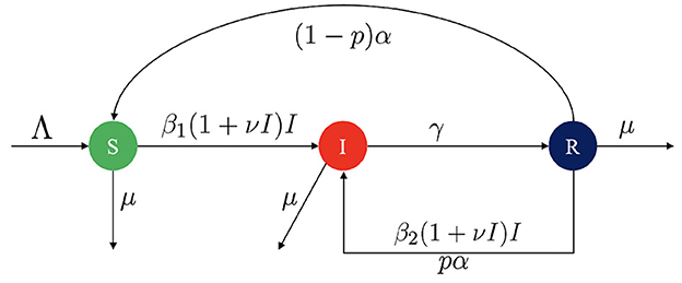
Figure 1. Transmission diagram for TB model in Equation 1.

Table 1

Table 1. Parameter description of TB model in Equation 2.

The population size increases with constant birth rate Λ and decreases only due to natural death rate μ. Vertical transmission of TB to a newborn from their mother are relatively rare [39, 40]. Hence, We assume that all newborns are susceptible to TB. Therefore, we have $\frac{dS}{dt}=\Lambda$ when we consider only the newborn factor. New infections arise from close contact between susceptible and infected individuals, with a constant infection rate, β₁. As the number of infected individuals in the population increases, TB spreads more easily within the community. Thus, rather than assuming a linear total contact rate represented by β₁I, we incorporate a nonlinear infection term. The infection risk for each susceptible individual is modeled as β₁(1 + νI)I, where ν is a correction parameter that captures the increased risk of TB spread when there is a larger infected population. A higher value of ν implies a greater ease of TB transmission. Infected individuals are assumed to recover at a constant rate γ.

This article also focuses on the effects of TB relapse and reinfection. In our model, relapse refers to the recurrence of active TB in individuals who were previously treated and considered cured, but who have a weakened immune system that allows the infection to return [26]. We assume that the period in which relapse is possible occurs at rate α, and that a proportion p of individuals in the recovered compartment may relapse. Hence, (1 − p)α represents the rate of individuals who recover completely without relapse.

Another factor in our model is the reinfection of recovered individuals. In TB, reinfection occurs when a previously cured individual becomes infected again with a new strain of Mycobacterium tuberculosis [26]. This reinfection is denoted using the term β₂. Following a similar approach as above, the reinfection risk for recovered individuals is represented by β₂(1 + νI).

Based on the above model description, the mathematical model of TB considering nonlinear incidence rate, relapse, and reinfection is given by:

$\begin{array}{l}{S}^{\prime }=\Lambda -{\beta }_1(1+\nu I)IS+(1-p)\alpha R-\mu S,\\ I^{\prime }={\beta }_1(1+\nu I)IS-\gamma I+p\alpha R+{\beta }_2(1+\nu I)IR-\mu I,\\ R^{\prime }=\gamma I-\alpha R-{\beta }_2(1+\nu I)IR-\mu R,& (1)\end{array}$

where

$S(0)\ge 0,I(0)>0,R(0)>0,\text{ and }N(0)=S(0)+I(0)+R(0).$

Since the total human population is constant, summing all equations in system Equation 1 gives:

$\frac{dN}{dt}=\Lambda -\mu N=0\iff \Lambda =\mu N.$

Next, let's assume

$x_1=\frac{S}{N},x_2=\frac{I}{N},x_3=\frac{R}{N},b_1={\beta }_{1}N,b_2={\beta }_{2}N,v=\nu N,$

and x₁ = 1 − x₂ − x₃, then the TB model in Equation 1 is reduced into the following two-dimensional model:

$\begin{array}{l}{x}_2^{\prime }=(b_1(1-x_2-x_3)+b_2{x}_3)(1+v{x}_2)x_2+p\alpha x_3-(\gamma +\mu )x_2,\\ x_3^{\prime }=\gamma x_2-b_2(1+v{x}_2)x_3{x}_2-(\alpha +\mu )x_3.& (2)\end{array}$

The non-dimension model in Equation 1 is equipped with a non-negative initial condition:

$x_2(0)>0,x_3(0)>0.$

Theorem 1. The non-dimension TB model in Equation 2 always gives a positive solution as long as the initial condition is non-negative.

Proof. In the boundary of ${ℝ}_{+}^2$, we have:

$x_2^{\prime }(x_2=0)=p\alpha x_3\ge 0,x_3^{\prime }(x_3=0)=\gamma x_2\ge 0.$

Since the initial condition is non-negative, all directions that tend to the boundary of ${ℝ}_{+}^2$ will be repelled back inside. Hence, As long as the initial condition is non-negative, the solution of x₂(t) and x₃(t) will always be non-negative in ${ℝ}_{+}^2$.     □

By Theorem 1, we can ensure that the solution of system (Equation 2) always has a biological interpretation, as the proportion of individuals relative to the total population remains positive. Also, since the total population is constant, x₂(t) + x₃(t) ≤ 1. In the next section, we will analyze the dynamic properties of the TB model in Equation 2.

3 Model analysis

In this section, we analyze our non-dimensionalized model in Equation 2 with respect to several key dynamical properties, including the existence criteria for equilibrium points, the calculation of the basic reproduction number, and the stability analysis of the equilibrium points. All calculations are performed both analytically and numerically.

3.1 TB-free equilibrium points and the basic reproduction number

There are two types of equilibrium points of system (Equation 2), i.e., the TB-free equilibrium point and the TB-endemic equilibrium point.

The TB-free equilibrium point of system (Equation 1) is given by:

$\begin{array}{ll}{\mathcal{E}}^{*}=(x_2^{*},x_3^{*})=(0,0).& (3)\end{array}$

Using the next-generation matrix approach given in Diekmann et al. [41], the basic reproduction number of system (Equation 2) is given by:

$\begin{array}{ll}{\mathcal{R}}_0=\frac{b_1}{\mu +\gamma }.& (4)\end{array}$

The basic reproduction number is a key epidemiological threshold that represents the expected number of secondary infections caused by a single infectious individual in a completely susceptible population. It is a threshold parameter used to determine the potential existence or extinction of a diseases among population. We further discuss the role of ${\mathcal{R}}_0$ in determining the existence and stability of equilibrium points in the following section.

3.2 TB-endemic equilibrium point

The second type of equilibrium point is the TB-endemic equilibrium point, which is given by:

$\begin{array}{ll}{\mathcal{E}}^{†}=(x_2^{†},x_3^{†}),& (5)\end{array}$

where $x_3^{†}=\frac{\gamma x_2^{†}}{b_2{x}_2(1+v{x}_2)+\alpha +\mu }$, while $x_2^{†}$ is taken from the positive roots of the following polynomial:

$\begin{array}{ll}f(x_2)=a_4{x}_2^4+a_3{x}_2^3+a_2{x}_2^2+a_1{x}_2+a_0=0,& (6)\end{array}$

with:

$\begin{array}{l}{a}_4=b_1{b}_2{v}^2>0,\\ a_3=b_1{b}_{2}v(2-v),\\ a_2=\alpha v{b}_1+\gamma v{b}_1+\mu v{b}_1+\mu v{b}_2-2v{b}_1{b}_2+b_1{b}_2,\\ a_1=-\alpha v{b}_1-\mu v{b}_1+b_1\alpha +\gamma b_1+b_1\mu +\mu b_2-b_1{b}_2,\\ a_0=-p\alpha \gamma +\alpha \gamma +\mu \alpha -b_1\alpha +\gamma \mu +{\mu }^2-b_1\mu .\end{array}$

The polynomial of f(x₂) is four degree. So, there could be more than one possible positive roots. Therefore, we analyzed the possible positive roots of f(x₂) using the Descartes rules of sign. The results of our analysis are given in Table 2 below.

Table 2

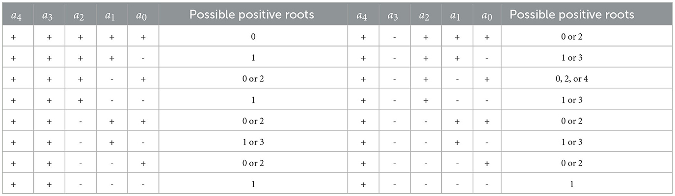
Table 2. Possible positive roots of f(x₂).

It can be seen from Table 2 that whenever a₀ < 0, f(λ) will always have at least one positive root. Solving ${\mathcal{R}}_0$ with respect to b₁ and substituting it into a₀, we will have:

$a_0=(\mu +\gamma )(\mu +\alpha )(1-{\mathcal{R}}_0)-p\alpha \gamma .$

Hence, we have

$a_0<0\iff {\mathcal{R}}_0>min\left\{1,{\mathcal{R}}_1\right\},$

where

$\begin{array}{ll}{\mathcal{R}}_1=1-\frac{p\alpha \gamma }{(\alpha +\mu )(\alpha +\gamma )}.& (7)\end{array}$

Since ${\mathcal{R}}_1<1$, then $min\left\{1,{\mathcal{R}}_1\right\}={\mathcal{R}}_1$. Based on the above calculation, we have the following theorem:

Theorem 2. The TB model in Equation 2 will always have at least one TB-endemic equilibrium if ${\mathcal{R}}_0>{\mathcal{R}}_1.$

To illustrate Theorem 2, let's assume [14, 15, 24]

$b_1=0.4,b_2=0.1,\mu =1/73,\gamma =1/2,p=0.5,\alpha =1/5,v=0.1.$

Using this data, we can determine

${\mathcal{R}}_0=0.778>min\left\{1,0.544\right\}=0.544.$

Hence, a TB endemic equilibrium exists, which is given by

$(x_2^{†},x_3^{†})=(0.105,0.234).$

Based on Theorem 2, we can conclude that ${\mathcal{R}}_0<1$ does not guarantee the non-existence of a TB endemic equilibrium. TB may still exist in the population even though ${\mathcal{R}}_0<1$.

3.3 Special case when v = 0, p = 0

For the first special case of model (Equation 2), we assume that the infection rate is linear with respect to I, which gives us v = 0, and no relapse occurred, which gives us p = 0. With this assumption, the model in Equation 2 can be reduced as follows:

$\begin{array}{l}{x}_2^{\prime }=(b_1(1-x_2-x_3)+b_2{x}_3)x_2-(\gamma +\mu )x_2,\\ x_3^{\prime }=\gamma x_2-b_2{x}_3{x}_2-(\alpha +\mu )x_3.& (8)\end{array}$

From the special case TB model in Equation 3, we can infer that the basic reproduction number is still the same as the complete model, which is ${\mathcal{R}}_0=\frac{b_1}{\mu +\gamma }.$ The TB-endemic equilibrium of model Equation 3 is given by

${\mathcal{E}}^{+}=(x_2^{+},x_3^{+}),$

where $x_3^{+}=\frac{\gamma x_2^{+}}{b_2{x}_2^{+}+\alpha +\mu }$, while $x_2^{+}$ is taken from the positive roots of the following two-degree polynomial:

$\begin{array}{l}g(x_2)=b_1{b}_2{x}_2^2+b_2(\mu -{\mathcal{R}}_0(\mu +\gamma ))+({\mathcal{R}}_0(\mu +\gamma )(\mu +\gamma +\alpha ))x_2\\ +(\mu +\alpha )(\mu +\gamma )(1-{\mathcal{R}}_0)=0.\end{array}$

It can be clearly seen that if ${\mathcal{R}}_0>1$, then the multiplication of the roots of g(x₂) = 0 will be negative, which indicates the appearance of a unique TB-endemic equilibrium if ${\mathcal{R}}_0>1$. Furthermore, if $\frac{\partial x_2}{\partial {\mathcal{R}}_0}<0$ at $x_2=0,{\mathcal{R}}_0=1$, then we will have positive roots for some interval at ${\mathcal{R}}_0<1$. From direct calculation, we have

$\frac{\partial x_2}{\partial {\mathcal{R}}_0}(x_2=0,{\mathcal{R}}_0=1)<0\leftrightarrow b_2^{*}=\frac{(\mu +\gamma )(\mu +\gamma +\alpha )}{\gamma }>1.$

Since g(x₂) is a two-degree polynomial, we will have two TB-endemic equilibria at ${\mathcal{R}}_0<1$ if ${\mathcal{R}}_1>1$ and ${\mathcal{R}}_0\in (\mathcal{K},1],$ where $\mathcal{K}$ is ${\mathcal{R}}_0$ that satisfies the discriminant of g(x₂) > 0. Based on this calculation, we have the following theorem.

Theorem 3. The special case of the TB model in Equation 3 has:

1. Unique TB-endemic equilibrium point if ${\mathcal{R}}_0>1$.

2. Twin TB-endemic equilibrium points at ${\mathcal{R}}_0=\mathcal{K}$ if $b_2^{*}>1$.

3. Two different TB-endemic equilibrium points at ${\mathcal{R}}_0\in (\mathcal{K},1]$ if $b_2^{*}>1$.

To illustrate Theorem 3, we use the following parameter values:

$\mu =1/73,\gamma =1/2,\alpha =1/10.$

With these parameter values, we obtain $b_2^{*}=0.63$ and $\mathcal{K}=0.44$. We consider two different values for b₂ to generate the equilibrium diagram shown in Figure 2, by selecting b₁ as the bifurcation parameter. The branching point BP is defined where ${\mathcal{R}}_0=1$, specifically at b₁ = 0.5136, while the fold point FP corresponds to $b_1=\mathcal{K}$, i.e., b₁ = 0.4416. In Figure 2a, we set $b_2=0.2<b_2^{*}$. Therefore, as per Theorem 3, when b₁ < BP, there is no TB-endemic equilibrium point, whereas if b₁ > BP, a unique TB-endemic equilibrium point arises. On the other hand, when $b_2=0.9>b_2^{*}$ as shown in Figure 2b, there is no endemic equilibrium if b₁ < 0.4416, a twin TB-endemic equilibrium point when b₁ = 0.4416, two distinct endemic equilibrium points for b₁ ∈ (0.4416, 0.5136), and a unique TB-endemic equilibrium point for b₁ ≥ 0.5136.

Figure 2

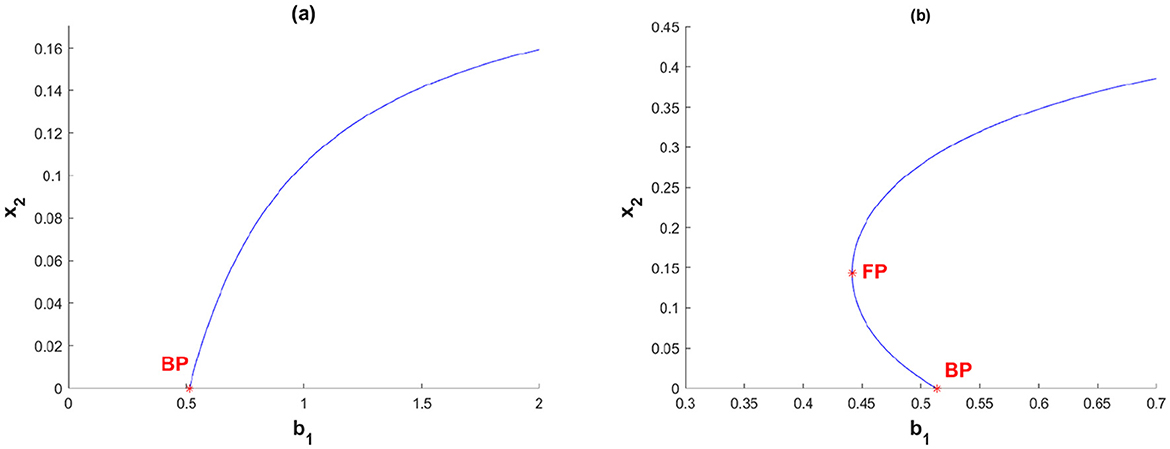
Figure 2. Equilibrium diagram of special case TB model in Equation 3 when (a) β₂ = 0.2 and (b) β₂ = 0.9.

3.4 Stability of TB-free equilibrium point

Linearizing system (Equation 2) in ${\mathcal{E}}^{*}$ gives:

$\begin{array}{ll}J({\mathcal{E}}^{*})=\left[\begin{array}{cc}{b}_1-\mu -\gamma & p\alpha \\ \gamma & -\alpha -\mu \end{array}\right].& (9)\end{array}$

Hence, the characteristic polynomial of $J({\mathcal{E}}^{*})$ is given by:

$\begin{array}{ll}h(\lambda )={\lambda }^2+c_1\lambda +c_0=0,& (10)\end{array}$

where c₁ = γ + α + 2μ − b₁ and $c_0=(\mu +\gamma )(\mu +\alpha )(1-{\mathcal{R}}_0)-p\alpha \gamma .$ Hence, h(λ) = 0 will give eigenvalues with negative real parts if c₀ > 0 and c₁ < 0. Therefore, we have the following theorem.

Theorem 4. The TB-free equilibrium point ${\mathcal{E}}^{*}$ of system (Equation 2) is locally asymptotically stable if ${\mathcal{R}}_0<{\mathcal{R}}_1.$

To illustrate Theorem Equation 4, we use the following parameter values:

$b_1=0.2,b_2=0.1,\mu =1/73,\gamma =1/2,p=0.5,\alpha =1/5,v=0.1,$

which gives

${\mathcal{R}}_0=0.389<min\left\{1,0.544\right\}=0.544.$

Then the TB-free equilibrium ${\mathcal{E}}^{*}=(0,0)$ is locally asymptotically stable since the eigenvalues are λ₁ = −0.49 and λ₂ = −0, 034.

3.5 Stability of TB-endemic equilibrium point

We conducted numerical experiments using MatCont to illustrate the stability of the endemic equilibrium point of TB model in Equation 2. MatCont is a MATLAB-based software package intended for numerical continuation and bifurcation analysis of dynamical systems. It is mostly employed in mathematical modeling to examine the behavior of differential equations, particularly for assessing the stability of equilibrium points and pinpointing bifurcation points in nonlinear systems.

Unless stated otherwise, we use the following parameter values:

$b_2=0.5,\mu =1/73,\gamma =1/2,p=0.5,\alpha =0.001$

with v varying and b₁ as the bifurcation parameter. Here, BP denotes the branching point and FP denotes the fold point. The first numerical experiment is illustrated in Figure 3 with v = 0.1. Figure 3 shows a forward bifurcation phenomenon, that as b₁ increases from 0, a stable TB-free equilibrium exists until it reaches the branching point BP at b₁ = 0.4966. At b₁ = 0.4966, the TB-free equilibrium shifts from a stable to an unstable equilibrium, while a unique TB-endemic equilibrium point begins to emerge. Figures 3a–c represent the bifurcation diagram in the b₁ − x₂ − x₃ space, the b₁ − x₂ plane, and the b₁ − x₃ plane, respectively.

Figure 3

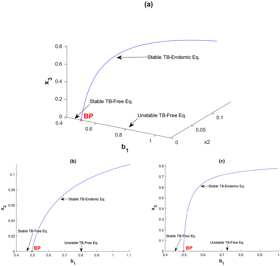
Figure 3. Forward bifurcation diagram of system (Equation 2) with v = 0.1 between (a) b₁ with x₂ and x₃, (b) b₁ with x₂, and (c) b₁ with x₃.

The second simulation in this section is shown in Figure 4, where we set v = 1.5. With this parameter configuration, the system exhibits a forward bifurcation, departing from the branch point BP at b₁ = 0.4966 and soon encountering its first fold point FP1 at b₁ = 0.4984. The TB-endemic equilibrium is stable as it leaves the branch point but loses stability upon reaching FP1. This unstable TB-endemic equilibrium continues to increase in backward direction as b₁ decreases along this branch until it reaches the second fold point FP2 at b₁ = 0.4425. When passing FP2, the TB-endemic equilibrium transitions from unstable to stable and remains stable for all subsequent values of b₁. From this simulation, we can define four intervals of b₁ based on the number and stability of the equilibria:

1. Interval 1: For b₁ < 0.4425, only the stable TB-free equilibrium point exists. The dynamics of x₂ for different initial conditions tends to a same TB-free equilibrium can be seen in Figure 5a.

2. Interval 2: For b₁ ∈ [0.4425, 0.4966], the TB-free equilibrium remains stable, the smaller TB-endemic equilibrium is unstable, and the larger TB-endemic equilibrium is stable. Thus, a bistability phenomenon occurs in this interval. The dynamics of x₂ for different initial conditions tends to a different equilibrium can be seen in Figure 5b.

3. Interval 3: For b₁ ∈ (0.4966, 0.4984], the TB-free equilibrium becomes unstable, but three TB-endemic equilibria exist, with the smallest and largest equilibria being stable and the middle one unstable. Bistability is also observed in this interval, with two stable TB-endemic equilibria appears. The dynamics of x₂ for different initial conditions tends to a different TB-endemic equilibrium can be seen in Figure 5c.

4. Interval 4: For b₁ > 0.4984, the TB-free equilibrium remains unstable, and the only remaining stable equilibrium is the TB-endemic equilibrium. The dynamics of x₂ for different initial conditions tends to a same TB-endemic equilibrium can be seen in Figure 5d.

Figure 4

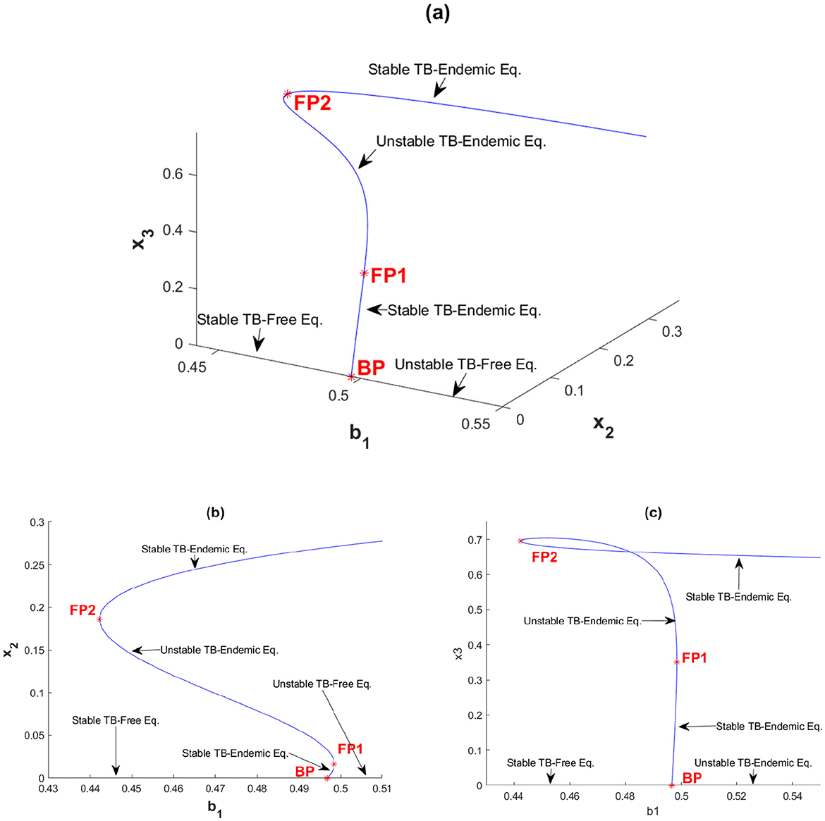
Figure 4. Forward bifurcation with hysteresis diagram of system (Equation 2) with v = 1.5 between (a) b₁ with x₂ and x₃, (b) b₁ with x₂, and (c) b₁ with x₃.

Figure 5

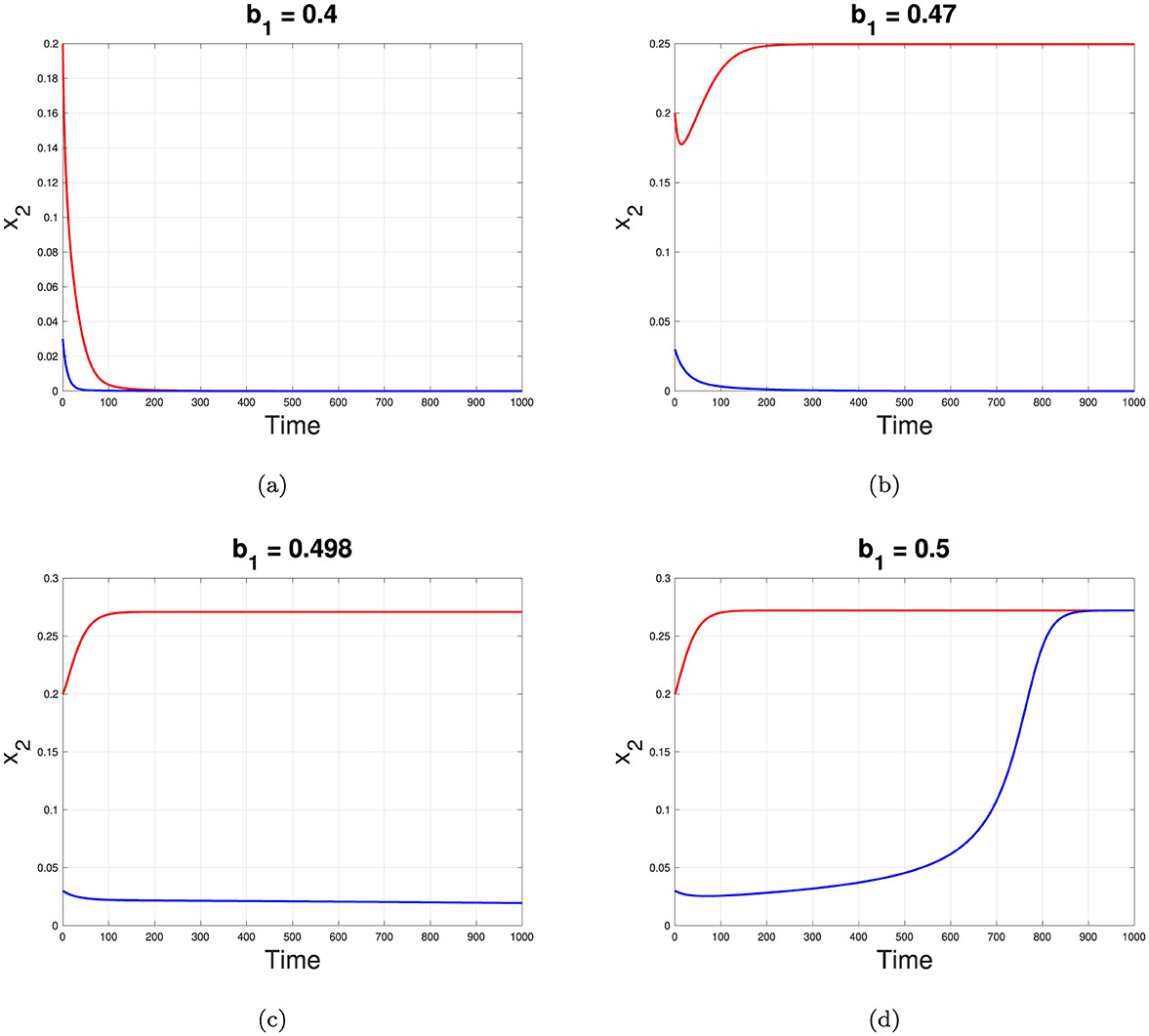
Figure 5. Dynamic of x₂ tends to it equilibrium depend on different value of b₁ correspond to interval 1, 2, 3, and 4 for (a–d), respectively.

This analysis reveals a rich structure of equilibrium behavior depending on the value of b₁ as an impact of v, including regions with bistability between TB-free and TB-endemic equilibrium points.

The next simulation is presented in Figure 6 with v = 2. Increasing v from 0.1 in Figure 3 to v = 2 in Figure 6 shifts the bifurcation diagram from forward to backward bifurcation. Backward bifurcation reveals a bistability phenomenon, where both TB-free and TB-endemic equilibrium points can coexist. Starting at b₁ = 0 and increasing b₁ in Figure 6b, a stable TB-free equilibrium persists until the branching point BP at b₁ = 0.4966. Beyond BP, the TB-free equilibrium becomes unstable, while a TB-endemic equilibrium point appears in the backward direction. For values of b₁ between 0.233 and 0.4966, an initial unstable TB-endemic equilibrium point emerges. Upon reaching the fold point FP, this TB-endemic equilibrium point adopts a stable asymptotic behavior, maintaining stability as b₁ continues to increase. Consequently, within the range b₁ ∈ (0.233, 0.4966), a bistability phenomenon occurs: a stable TB-free equilibrium exists and two TB-endemic equilibria are present, with the smaller equilibrium being unstable and the larger one being stable.

Figure 6

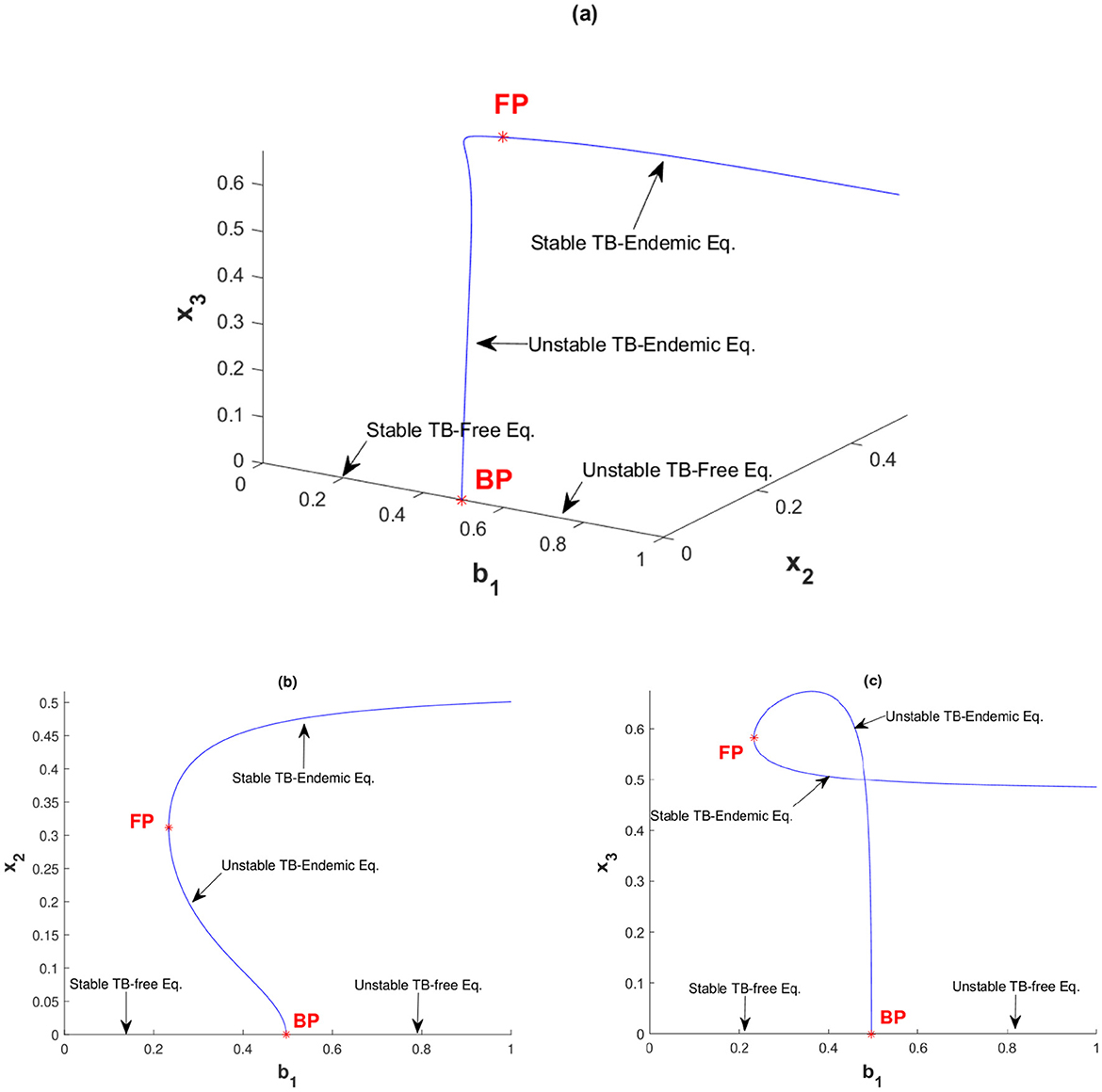
Figure 6. Backward bifurcation diagram of system (Equation 2) with v = 2 between (a) b₁ with x₂ and x₃, (b) b₁ with x₂, and (c) b₁ with x₃.

4 Sensitivity analysis

4.1 Global sensitivity analysis

To better understand the impact of relapse, reinfection, and nonlinear incidence rate on the dynamics of TB within our proposed model in Equation 2, we performed a global sensitivity analysis on the dynamics of the proportion of infected individuals, x₂. We used a combination of Latin Hypercube Sampling (LHS) and Partial Rank Correlation Coefficient (PRCC) to pick 5000 samples for this global sensitivity analysis. The results of this analysis are presented in Figure 7. Through this simulation, we can identify the parameters that most significantly affect the dynamics of x₂.

Figure 7

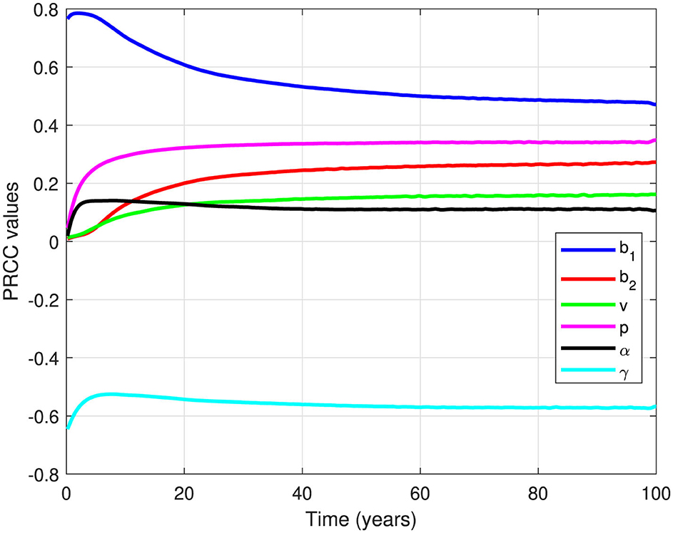
Figure 7. PRCC values for all parameters (except μ) when measured against the dynamics of infected individuals over time.

It is clear from Figure 7 that all parameters in Equation 2 have positive PRCC values, except γ. Therefore, an increase in b₁, b₂, v, p, and α will result in an increase in the number of infected individuals. In other words, an increase in the infection rate, reinfection rate, relapse rate, proportion of relapse, and correction parameter for nonlinear incidence rate would all contribute to increasing the number of infected individuals. In contrast, an increase in the natural recovery rate γ will reduce the number of infected individuals.

An additional insight from Figure 7 is that b₁ is the most influential parameter on the dynamics of x₂, followed by γ, p, b₂, v, and α, respectively. Therefore, the most impactful interventions to control the number of infected individuals would involve reducing b₁ or increasing γ. This could be achieved by minimizing primary infections through measures like utilization of face masks, vaccinations, or any prevention strategy that reduces b₁, or by improving the TB recovery rate through better medication or by reducing treatment failure rates through Directly Observed Therapy (DOT).

The following global sensitivity analysis focuses on the stability threshold of the TB-free equilibrium from Theorem 4. According to Theorem 4, the TB-free equilibrium point is locally stable if ${\mathcal{R}}_0<{\mathcal{R}}_1$, or equivalently if

${\mathcal{R}}_2=\frac{{\mathcal{R}}_0}{{\mathcal{R}}_1}=\frac{b_1(\alpha +\mu )}{\mu (\mu +\alpha +\gamma )+(1-p)\alpha \gamma }<1.$

The next global sensitivity analysis examines the impact of parameter values on model (Equation 2) with respect to ${\mathcal{R}}_2$. Notably, only the parameters b₁, p, α, γ, and μ appear in ${\mathcal{R}}_2$, while b₂ and v do not. This indicates that b₂ and v do not determine the stability of the TB-free equilibrium; however, they can affect the magnitude of x_i at the endemic equilibrium point. The global sensitivity analysis results for ${\mathcal{R}}_2$ are presented in Figure 8. As shown in Figure 8a, among the studied parameters, γ has the maximum influence on ${\mathcal{R}}_2$, followed by p, b₁, and α. The distribution of ${\mathcal{R}}_2$ based on the samples used in Figure 8a is illustrated in Figure 8b, where most frequencies of ${\mathcal{R}}_2$ are concentrated below 1.

Figure 8

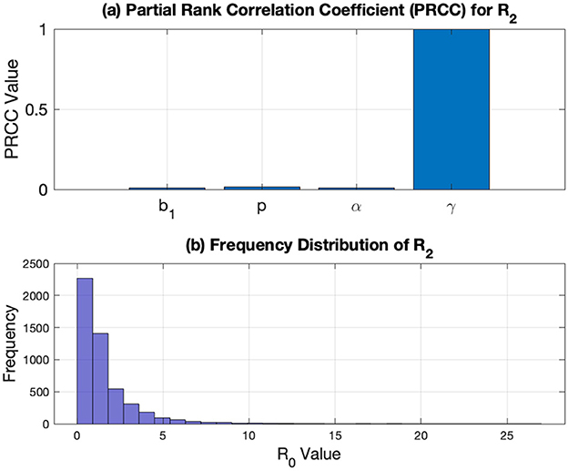
Figure 8. (a) PRCC results on ${\mathcal{R}}_2$ and (b) the distribution of ${\mathcal{R}}_2$ using samples used on PRCC.

4.2 Two-parameter sensitivity analysis

From previous global sensitivity analysis, it can be seen that b₁ is the most sensitive parameter on the dynamic of infected individuals. Hence, it is essential to analyze the effect of b₁ and other parameters on the stability of the TB-free equilibrium point.

The first numerical experiment is given in Figure 9a, where we depict the sensitivity of ${\mathcal{R}}_2$ with respect to b₁ and p. It is clearly seen that an increase in the number of primary infections and the proportion of people getting relapses will increase ${\mathcal{R}}_2$. The second simulation depicted in Figure 9b shows how the combination of α and γ affect ${\mathcal{R}}_2$. It can be clearly seen that increasing α will increase ${\mathcal{R}}_2$, while reducing γ will reduce ${\mathcal{R}}_2$. Hence, increasing the natural recovery rate of TB can increase the chances of TB elimination efforts.

Figure 9

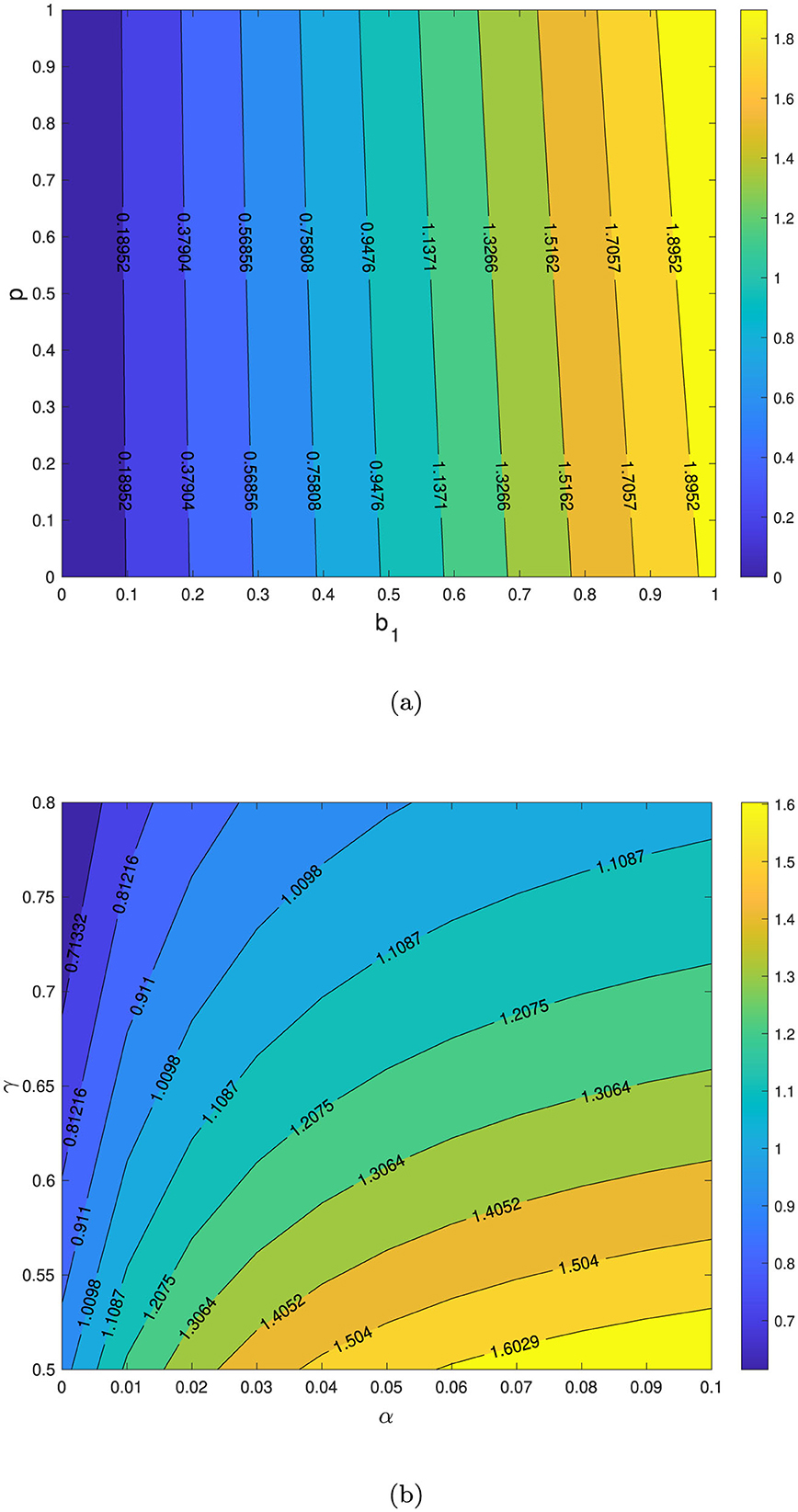
Figure 9. Contour plot of ${\mathcal{R}}_2$ with respect to b₁ vs. p in (a) and α vs. γ in (b). TB-free equilibrium will be stable if ${\mathcal{R}}_2<1$.

4.3 Autonomous simulation

In this section, we conducted numerical experiments to explore the dynamics of x₂ in response to variations in parameter values. The baseline parameters were set as follows:

$b_1=0.5,b_2=0.5,\mu =1/73,\gamma =1/2,p=0.5,\alpha =0.001,v=1.5,$

unless specified otherwise. The time frame for simulation is varying to expose the dynamic of x₂. Results are shown in Figure 10.

Figure 10

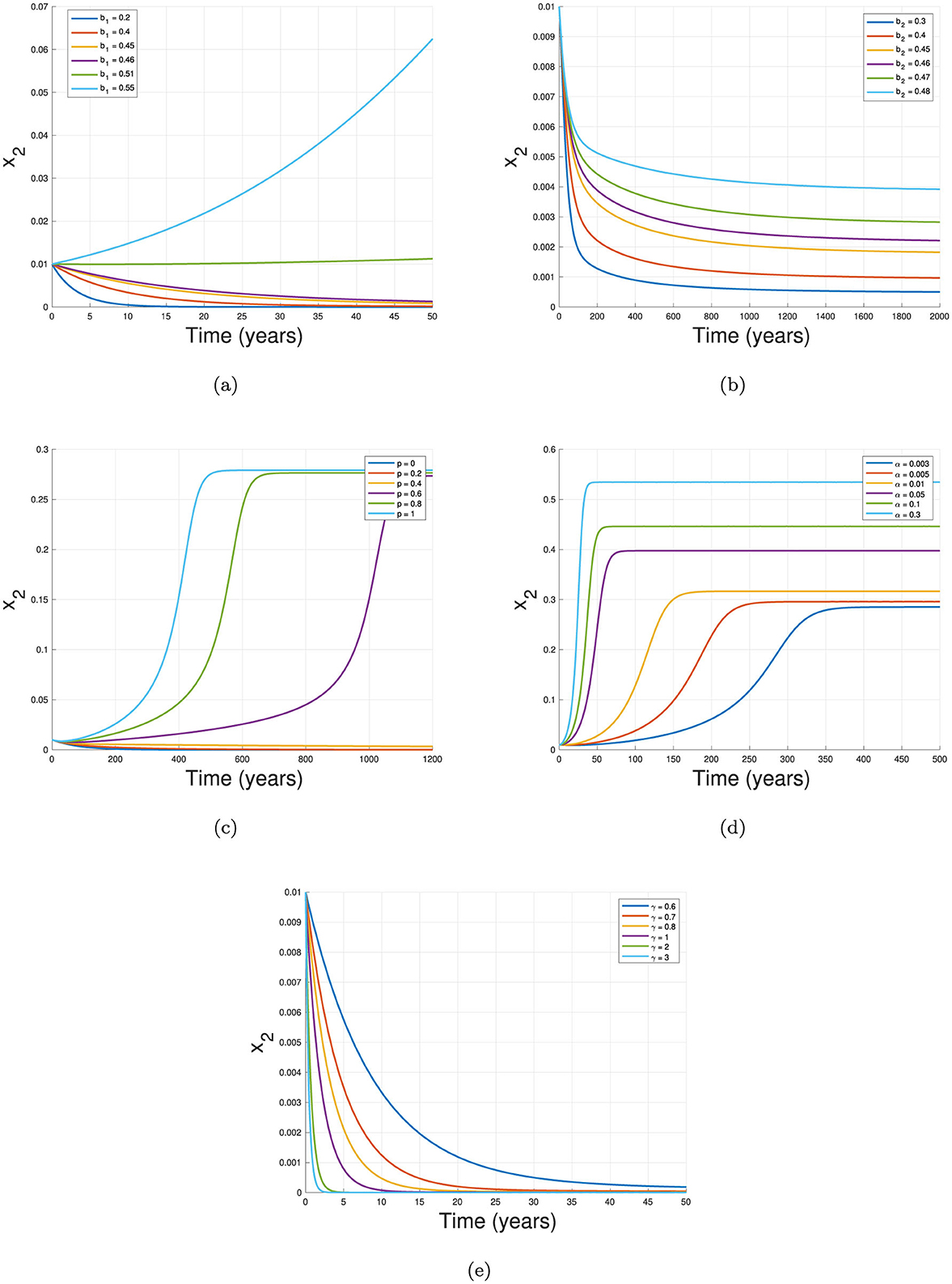
Figure 10. Sensitivity on the dynamics of x₂ with respect to (a) b₁, (b) b₂, (c) ρ, (d) α, and (e) γ.

The first experiment, shown in Figure 10a, illustrates the effect of the primary infection rate, b₁, on the dynamics of x₂. Holding all other parameters constant, we observe that higher TB primary infection rates lead to a larger number of infected individuals and prolong the outbreak. Figure 10b similarly demonstrates that increasing the reinfection parameter, b₂, also raises infection levels.

In Figure 10c, we examine the effect of the proportion of individuals experiencing relapse, p. With no relapse (p = 0), x₂ directly tends to it TB-free equilibrium faster than case of p = 0.2 and p = 0.4. On the other hand, when p = 0.6, 0.8, and 1, the dynamic of x₂ increasing significantly and tends to it TB-endemic equilibrium. Figure 10d highlights the impact of the relapse rate, α, where higher values of α correlate with a larger infected population. This finding is intuitive, as a lower relapse rate means a larger reservoir of individuals, x₃, who are susceptible to reinfection. Thus, when this recovered group remains high due to a smaller α, reinfection events occur more frequently, increasing x₂.

The final simulation, shown in Figure 10e, examines the effect of the recovery rate, γ, on x₂ dynamics. Here, higher recovery rates significantly decrease x₂ levels and expedite outbreak control. This underscores the importance of rapid recovery in curbing disease transmission and achieving stability within the population.

4.4 Impact of infection rate adjustments: intensity, timing, and duration analysis

In many cases in the field, the intervention to control the spread of diseases depends on time. The duration of the intervention also adapts to the current situation or depends on budget limitations. Hence, in many cases, if intervention needs to be implemented, the duration of this intervention sometimes only takes a short time period for implementation. Based on this argument, here in this section we introduce a possible time-dependent infection rate b₁(t) which will depend on the intensity, timing of implementation, and duration of implementation. Reducing b₁ in TB spread can be related to any prevention strategy to avoid contact with infected individuals, such as the use of face masks. Hence, we define our adjusted b₁(t) as follows:

$\begin{array}{ll}{b}_1(t)=\{\begin{array}{ll}\theta & t_1\le t\le t_2\\ 0.47& \text{else}\end{array},& (11)\end{array}$

where t₁ is the first day of control measurement, t₂ is the last day of control measurement, and θ is the reduced infection rate b₁. Hence, we have three variables derived from the adjusted b₁ in Equation 11. The first variable is θ, which describes the intensity of the control measures to reduce the infection rate b₁. The second variable is the first day of intervention, denoted as t₁. A smaller t₁ indicates that the intervention was implemented earlier. The last variable is the duration of the intervention, given by $\bar{T}=t_2-t_1>0$. A larger $\bar{T}$ indicates a longer period of intervention.

For this simulation, we use the baseline parameters to produce Figure 5b with the initial condition represented by the red curve. In this case, bistability appears in the TB model, where the solution depends on the initial condition. In the red curve, where the initial number of infected individuals is larger, the trajectories tend to the TB-endemic equilibrium point. Conversely, with a smaller initial condition for x₂, the solution tends to the TB-free equilibrium point. The goal is to find the appropriate values of θ, t₁, or $\bar{T}$ such that the trajectories can change from the TB-endemic equilibrium to the TB-free equilibrium point.

We conduct four type of scenario to analyze the possible adjustment of b₁. The function of b₁ is given in Equation 11 with the value of θ, t₁, and t₂ is given in Table 3.

Table 3

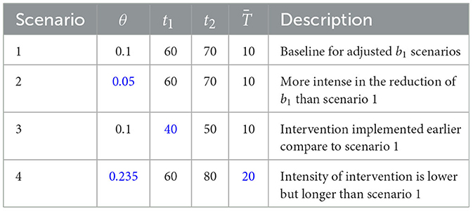
Table 3. Description of scenarios for adjusted b₁, where blue text indicates changes of strategy compared to scenario 1.

The result for the first scenario is shown in Figure 11a. It can be seen that when the infection rate is reduced from 0.47 to 0.1 starting from t = 60 for 10 years, the dynamics of the infected compartment x₂ decline until the end of the 70^th year and then begin to increase again, tending toward the TB-endemic equilibrium as the intervention is lifted. Thus, the effort in the first scenario does not succeed in pushing the trajectories of x₂ from the TB-endemic to the TB-free equilibrium point.

Figure 11

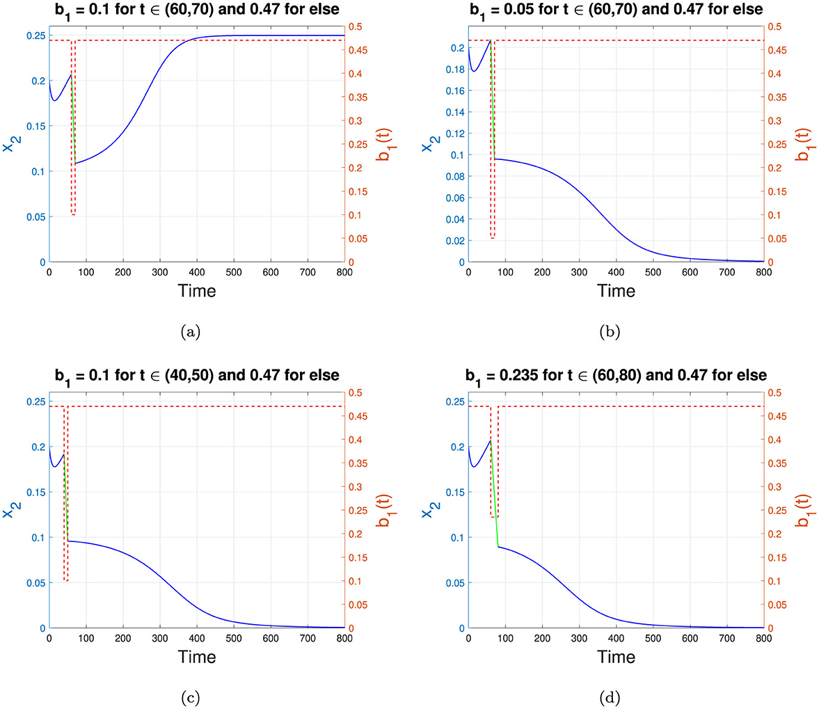
Figure 11. Changes in the trajectories of x₂ depend on the adjusted b₁. (a–d) represent scenarios 1 to 4 in Table 3, respectively. The blue and green curves represent the dynamics of x₂, while the red dotted curve shows the value of b₁ as a step function. The left y-axis corresponds to x₂, while the right y-axis corresponds to the value of b₁. The time scale is in years.

The second numerical simulation is conducted with the same setup as in scenario 1, but with a higher intensity of intervention such that b₁ is reduced from 0.47 to only 0.05. The result is shown in Figure 11b. Unlike scenario 1, with a higher intensity of reduction in b₁, we can push the trajectories of x₂ from the TB-endemic equilibrium to the TB-free equilibrium. Even when the intervention ends at the end of year 70, the trajectories of x₂ do not return to their natural path toward the TB-endemic equilibrium. Instead, it tend toward the TB-free equilibrium point. Hence, in this example, we can conclude that a sufficiently intense intervention can shift the solution trajectories from the TB-endemic to the TB-free equilibrium, even if the duration of the intervention remains the same.

The third scenario is conducted in the same manner as scenario 1, but with the intervention implemented earlier, specifically in the 40^th year. The duration and intensity of intervention remain the same as in scenario 1. The result is shown in Figure 11c. It can be seen that when the intervention is implemented 10 years earlier than in scenario 1, the solution trajectories can be pushed toward the TB-free equilibrium point. Therefore, determining the appropriate timing for the start of the intervention is essential to achieve a TB-free equilibrium in the population.

The fourth simulation is conducted for scenario 4. In many cases of disease control strategy, maintaining an intervention over a longer period is more feasible than applying a higher intensity to reduce the infection rate. In scenario 4, we illustrate this by reducing b₁ by only 50%, to 0.235, while assuming that the government can sustain this intervention for a longer period–in this case, 20 years. The result is shown in Figure 11d. It is clear that when the intervention can be maintained for a longer duration, the intensity of reduction does not need to be at the highest level to achieve a TB-free equilibrium. Thus, identifying an optimal duration for intervention and the minimum reduction in infection rate can enhance the effectiveness of TB elimination efforts.

4.5 Impact of recovery rate adjustments: intensity, timing, and duration analysis

Another potential intervention for the TB control program that can be analyzed using our proposed model is enhancing the recovery rate of infected individuals. This can be achieved through various measures, such as improving the quality of treatment or increasing the number of medical staff available to care for TB-infected individuals in hospitals. Similar approaches were implemented during the global COVID-19 outbreak from 2020 to 2022.

The concept behind this type of scenario is similar to that discussed in the previous section, where we define γ = γ(t), where:

$\begin{array}{ll}\gamma (t)=\{\begin{array}{ll}\zeta & t_1\le t\le t_2\\ 0.5& \text{else}\end{array}.& (12)\end{array}$

Here, ζ > 0.5 represents the improved value of the natural recovery rate achieved through government interventions using the aforementioned strategies. In this article, we implement four different strategies for defining γ(t), as shown in Table 4.

Table 4

Table 4. Description of scenarios for adjusted γ, where blue text indicates changes of strategy compared to scenario 1.

The numerical results for the first scenario in Table 4 are shown in Figure 12a. It can be observed that increasing the recovery rate by 10%, from 0.5 to 0.55, during t ∈ [60, 70] does not succeed in shifting the stability from the TB-endemic equilibrium to the TB-free equilibrium point. Although the recovery rate improvement significantly reduces the number of infected individuals during t ∈ [60, 70], the number of infected individuals begins to rise again and returns to the stable endemic equilibrium immediately after the recovery rate enhancement ceases. However, when the recovery rate is increased by 20% over the same time interval as in Scenario 1, Figure 12b shows that the dynamics of x₂ shift from the TB-endemic equilibrium to the TB-free equilibrium. In Scenario 3, represented in Figure 12c, the improvement of γ occurs earlier than in Scenario 1, specifically during t ∈ [40, 50]. It can be seen that these interventions do not succeed in shifting the stability to the TB-free equilibrium. Conversely, when the intervention is implemented over a longer period, as shown in Scenario 4, the stability successfully transitions from the TB-endemic to the TB-free equilibrium. The numerical results for Scenario 4 are illustrated in Figure 12d.

Figure 12

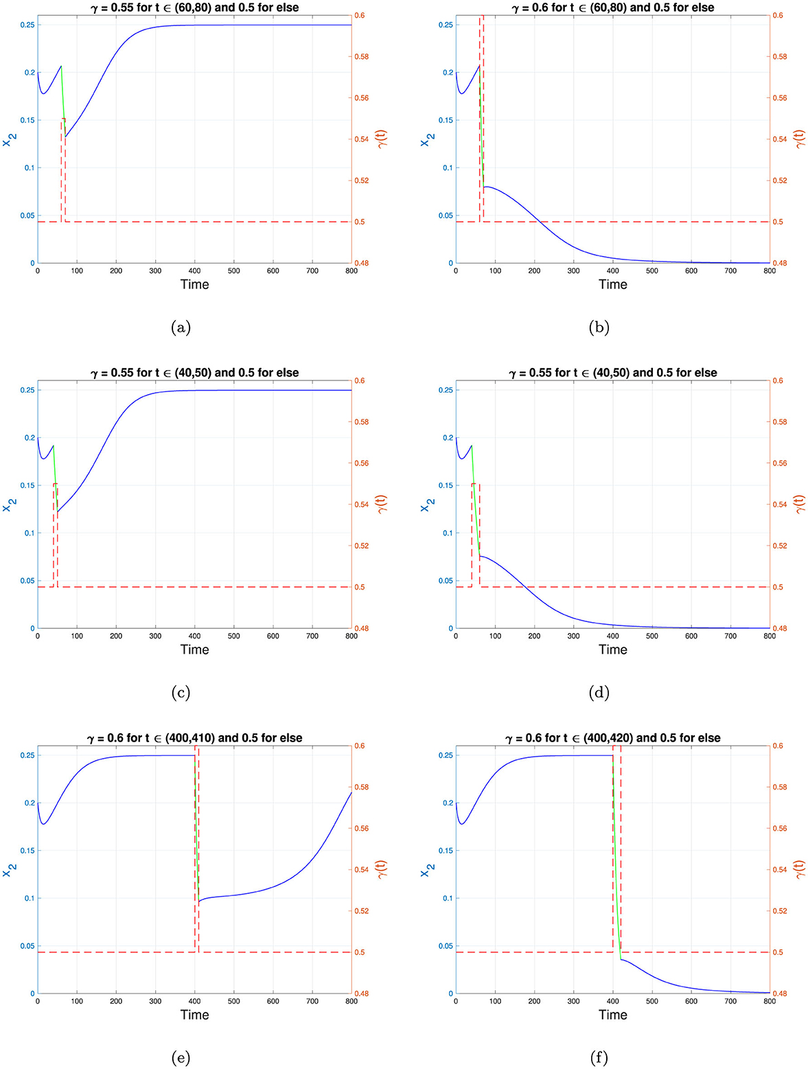
Figure 12. Changes in the trajectories of x₂ depend on the adjusted γ. (a–f) represent scenarios 1 to 6 in Table 4, respectively. The blue and green curves represent the dynamics of x₂, while the red dotted curve shows the value of γ as a step function. The left y-axis corresponds to x₂, while the right y-axis corresponds to the value of γ. The time scale is in years.

The fifth simulation describes a scenario where the intervention is introduced very late, at a point when the dynamics of x₂ are already approaching the TB-endemic equilibrium. In this case, the recovery rate γ is increased from 0.5 to 0.6, but the intervention is implemented late, during the interval t ∈ [400, 410]. The results, depicted in Figure 12e, indicate that while the dynamics of x₂ decrease during the intervention, they rise again to the TB-endemic equilibrium immediately after γ reverts to 0.5. However, when the same recovery rate improvement is applied at the same starting point but over a longer period, as in Scenario 6, the dynamics of x₂ shift to the TB-free equilibrium, as shown in Figure 12f.

From the numerical experiments involving γ, as defined in Equation 12, it is evident that improving the recovery rate requires appropriate intensity, timing, and duration of interventions. A carefully adjusted γ can redirect the dynamics of the infected population from the TB-endemic equilibrium to the TB-free equilibrium when bistability phenomena occur.

5 Conclusion

Mathematical models of tuberculosis transmission have been extensively studied by many researchers, incorporating key factors such as vaccination, quarantine, treatment, slow-fast disease progression, co-infection with other diseases, and more [42–47]. However, to the best of our knowledge, only few TB models consider the impact of population ignorance regarding the dangers of TB. Unlike COVID-19, which prompted high awareness early in the 2019 pandemic, TB has existed for decades, leading to a comparatively lower level of public awareness about its risks compared to newly emerging diseases like COVID-19.

In this paper, we have proposed a mathematical model to predict Tuberculosis (TB) transmission that considers a nonlinear incidence rate to capture the population's low awareness response to TB transmission, as well as relapse and reinfection. First, we non-dimensionalized the model and reduced it from a three- to a two-dimensional system by assuming a constant population over time. Using this non-dimensionalized model, we analyzed the dynamic behavior of the system with respect to the existence and local stability of equilibria. We identified two types of equilibrium points: the TB-free equilibrium and the TB-endemic equilibrium. Our findings suggest that a basic reproduction number less than one is not sufficient to ensure TB eradication; the reproduction number must be lower than a new threshold, which we denote as ${\mathcal{R}}_1$. Our analysis also reveals that the model may exhibit multiple TB-endemic equilibria, making TB eradication more challenging. The model demonstrates three types of bifurcation: forward bifurcation, backward bifurcation, and forward bifurcation with hysteresis. For more examples on TB transmission model which produced complex bifurcation phenomena, readers may refer to Aldila et al. [26].

A global sensitivity analysis, using a combination of Latin Hypercube Sampling (LHS) and Partial Rank Correlation Coefficient (PRCC), was conducted to identify the most influential parameters in our TB model. This analysis revealed that primary infection and recovery rates are the most significant parameters impacting the dynamics of the proportion of infected individuals. Moreover, although reinfection and the nonlinear incidence rate parameter do not appear in the endemic threshold, they exhibit significant positive PRCC values in relation to the dynamics of infected individuals. This finding highlights the importance of controlling reinfection and shaping population perspectives on TB to achieve more effective results in TB eradication.

In the final numerical experiment with an adjustable infection rate, we have demonstrated a potential strategy for TB eradication when bistability occurs–that is, when both the TB-free and TB-endemic equilibrium points are stable simultaneously. Our results indicate that if the intervention cannot be maintained indefinitely, careful consideration must be given to the intensity of the intervention (i.e., the reduction in infection rate), the timing of intervention (i.e., when it should begin), and the duration of intervention. When implemented appropriately, these factors can shift the system from a TB-endemic to a TB-free equilibrium. This highlights the importance of strategic, time-sensitive interventions in TB control, especially in settings where both TB-endemic and TB-free situation are possible outcomes. From a public health standpoint, this results shows how optimizing intervention intensity, timing, and duration is crucial to achieving sustained reductions in TB prevalence, ultimately moving toward eradication even when resources are limited.

In this paper, we have introduced a modified Susceptible-Infected-Recovered (SIR) model for TB transmission. Despite its simplicity, the model accommodates the key factors in TB transmission, such as relapse and reinfection. The results highlight the importance of relapse and reinfection as hidden parameters that do not appear in the basic reproduction number but significantly influence infection dynamics. However, our model has room for further improvement. Incorporating vaccination and its imperfect effects could be a direction for future work, given that vaccination is a critical TB control strategy. Additionally, modeling resistance to TB drugs (multi-drug resistance) could add further detail to the model.

Data availability statement

The original contributions presented in the study are included in the article/supplementary material, further inquiries can be directed to the corresponding author.

Author contributions

DA: Conceptualization, Data curation, Formal analysis, Funding acquisition, Investigation, Methodology, Project administration, Resources, Software, Supervision, Validation, Visualization, Writing – original draft, Writing – review & editing.

Funding

The author(s) declare that financial support was received for the research and/or publication of this article. This research was funded by the Ministry of Research and Higher Education, Republic of Indonesia with Fundamental Research Grant Scheme 2024 (ID Number: NKB-894/UN2.RST/HKP.05.00/2024).

Conflict of interest

The author declares that the research was conducted in the absence of any commercial or financial relationships that could be construed as a potential conflict of interest.

Generative AI statement

The author(s) declare that no Gen AI was used in the creation of this manuscript.

Publisher's note

All claims expressed in this article are solely those of the authors and do not necessarily represent those of their affiliated organizations, or those of the publisher, the editors and the reviewers. Any product that may be evaluated in this article, or claim that may be made by its manufacturer, is not guaranteed or endorsed by the publisher.

References

1. Chukwu C, Bonyah E, Juga M, et al. On mathematical modeling of fractional-order stochastic for tuberculosis transmission dynamics. Results Control Optim. (2023) 11:100238. doi: 10.1016/j.rico.2023.100238

Crossref Full Text | Google Scholar

2. Centers for Disease Control and Prevention. Signs and Symptoms of Tuberculosis (2024). Available online at: https://www.cdc.gov/tb/signs-symptoms/?CDC_AAref_Val=https://www.cdc.gov/tb/topic/basics/signsandsymptoms.htm (accessed May 10, 2024).

Google Scholar

3. Aldila D, Fardian B, Chukwu C, Noor Aziz MH, Kamalia P. Improving tuberculosis control: assessing the value of medical masks and case detection–a multi-country study with cost-effectiveness analysis. R Soc Open Sci. (2021) 8:210507.

PubMed Abstract | Google Scholar

4. WHO. Global Tuberculosis Report 2020 (2020). Available online at: https://www.who.int/publications/i/item/9789240013131 (accessed May 15, 2024).

Google Scholar

5. Barry CE, Boshoff HI, Dartois V, Dick T, Ehrt S, Flynn D, et al. The spectrum of latent tuberculosis: rethinking the biology and intervention strategies. Nat Rev Microbiol. (2009) 7:845–55. doi: 10.1038/nrmicro2236

PubMed Abstract | Crossref Full Text | Google Scholar

6. Mathema B, Kurepina NE, Bifani PJ, Kreiswirth BN. Molecular epidemiology of tuberculosis: current insights. Clin Microbiol Rev. (2006) 19:658–86. doi: 10.1128/CMR.00061-05

PubMed Abstract | Crossref Full Text | Google Scholar

7. Crampine A C. Recurrent TB: relapse or reinfection? The effect of HIV in a general population cohort in Malawi. Epidemiol Soc. (2010) 24:417–426. doi: 10.1097/QAD.0b013e32832f51cf

PubMed Abstract | Crossref Full Text | Google Scholar

8. Shen X, Yang C, Wu J, Lin S, Gao X, Wu Z, et al. Recurrent tuberculosis in an urban area in China: Relapse or exogenous reinfection? Tuberculosis. (2017) 103:97–104. doi: 10.1016/j.tube.2017.01.007

PubMed Abstract | Crossref Full Text | Google Scholar

9. Aldila D, Aulia Puspadani C, Rusin R. Mathematical analysis of the impact of community ignorance on the population dynamics of dengue. Front Appl Mathem Statist. (2023) 9:1094971. doi: 10.3389/fams.2023.1094971

Crossref Full Text | Google Scholar

10. Abidemi A, Fatmawati, Peter OJ. An optimal control model for dengue dynamics with asymptomatic, isolation, and vigilant compartments. Dec Anal J. (2024) 10:100413. doi: 10.1016/j.dajour.2024.100413

Crossref Full Text | Google Scholar

11. Handari BD, Ramadhani RA, Chukwu CW, Khoshnaw SHA, Aldila D. An optimal control model to understand the potential impact of the new vaccine and transmission-blocking drugs for malaria: a case study in Papua and West Papua, Indonesia. Vaccines. (2022) 10:1174. doi: 10.3390/vaccines10081174

PubMed Abstract | Crossref Full Text | Google Scholar

12. Febiriana IH, Hassan AH, Aldila D. Enhancing malaria control strategy: optimal control and cost-effectiveness analysis on the impact of vector bias on the efficacy of mosquito repellent and hospitalization. J Appl Mathem. (2024) 2024:9943698. doi: 10.1155/2024/9943698

Crossref Full Text | Google Scholar

13. Aldila D, Awdinda N, Fatmawati, Herdicho FF, Ndii MZ, Chukwu CW. Optimal control of pneumonia transmission model with seasonal factor: Learning from Jakarta incidence data. Heliyon. (2023) 9:e18096. doi: 10.1016/j.heliyon.2023.e18096

PubMed Abstract | Crossref Full Text | Google Scholar

14. Aldila D, Fardian BL, Chukwu CW, Hifzhudin Noor Aziz M, Kamalia PZ. Improving tuberculosis control: assessing the value of medical masks and case detection–a multi-country study with cost-effectiveness analysis. R Soc Open Sci. (2024) 11:231715. doi: 10.1098/rsos.231715

PubMed Abstract | Crossref Full Text | Google Scholar

15. Ginting EDA, Aldila D, Febiriana IH. A deterministic compartment model for analyzing tuberculosis dynamics considering vaccination and reinfection. Healthcare Anal. (2024) 5:100341. doi: 10.1016/j.health.2024.100341

Crossref Full Text | Google Scholar

16. Belabbas M, Souna F, Tiwari PK, Menacer Y. Role of intervention strategies and psychological effect on the control of infectious diseases in the random environment. J Biol Syst. (2024) 32:971–1001. doi: 10.1142/S0218339024500402

Crossref Full Text | Google Scholar

17. Mondal J, Samui P, Chatterjee AN, Ahmad B. Modeling hepatocyte apoptosis in chronic HCV infection with impulsive drug control. Appl Math Model. (2024) 136:115625. doi: 10.1016/j.apm.2024.07.032

Crossref Full Text | Google Scholar

18. Roy PK, Chatterjee AN Li XZ. The effect of vaccination to dendritic cell and immune cell interaction in HIV disease progression. Int J Biomathem. (2016) 09:1650005. doi: 10.1142/S1793524516500054

Crossref Full Text | Google Scholar

19. Wang B, Mondal J, Samui P, Chatterjee AN, Yusuf A. Effect of an antiviral drug control and its variable order fractional network in host COVID-19 kinetics. Eur Phys J Special Topics. (2022) 231:1915–29. doi: 10.1140/epjs/s11734-022-00454-4

PubMed Abstract | Crossref Full Text | Google Scholar

20. Rai RK, Pal KK, Tiwari PK, Martcheva M, Misra AK. Impact of social media and word-of-mouth on the transmission dynamics of communicable and non-communicable diseases. Int J Biomathem. (2024) 2024:2450094. doi: 10.1142/S1793524524500943

Crossref Full Text | Google Scholar

21. Pal KK, Rai RK, Tiwari PK. Influences of media-induced awareness and sanitation practices on cholera epidemic: a study of bifurcation and optimal control. Int J Bifurc Chaos. (2024) 2024:2550002. doi: 10.1142/S0218127425500026

Crossref Full Text | Google Scholar

22. Simorangkir G, Aldila D, Rizka A, Tasman H, Nugraha ES. Mathematical model of tuberculosis considering observed treatment and vaccination interventions. J Interdisc Mathem. (2021) 24:1717–37. doi: 10.1080/09720502.2021.1958515

Crossref Full Text | Google Scholar

23. Kamalia PZ, Ayumi T, Fathiyah AY, Aldila D. Global stability analysis and optimal control problem arise from tuberculosis transmission model with monitored treatment. Commun Math Biol Neurosci. (2024) 15:27.

Google Scholar

24. Aldila D, Ramadhan DA, Chukwu CW, Handari BD, Shahzad M, Kamalia PZ. On the role of early case detection and treatment failure in controlling tuberculosis transmission: a mathematical modeling study. Commun Biomathem Sci. (2024) 7:61–86. doi: 10.5614/cbms.2024.7.1.4

Crossref Full Text | Google Scholar

25. Aldila D, Saslia BR, Gayarti W, Tasman H. Backward bifurcation analysis on Tuberculosis disease transmission with saturated treatment. J Phys. (2021) 1821:012002. doi: 10.1088/1742-6596/1821/1/012002

PubMed Abstract | Crossref Full Text | Google Scholar

26. Aldila D, Chavez JP, Wijaya KP, Ganegoda NC, Simorangkir GM, Tasman H, et al. A tuberculosis epidemic model as a proxy for the assessment of the novel M72/AS01E vaccine. Commun Nonl Sci Numer Simulat. (2023) 120:107162. doi: 10.1016/j.cnsns.2023.107162

Crossref Full Text | Google Scholar

27. Bhunu CP. Mathematical analysis of a three-strain tuberculosis transmission model. Appl Math Model. (2011) 35:4647–60. doi: 10.1016/j.apm.2011.03.037

Crossref Full Text | Google Scholar

28. Sergeev R, Colijn C, Cohen T. Models to understand the population-level impact of mixed strain M. tuberculosis infections. J Theor Biol. (2011) 280:88–100. doi: 10.1016/j.jtbi.2011.04.011

PubMed Abstract | Crossref Full Text | Google Scholar

29. Omede BI, Peter OJ, Atokolo W, Bolaji B, Ayoola TA. A mathematical analysis of the two-strain tuberculosis model dynamics with exogenous re-infection. Healthcare Anal. (2023) 4:100266. doi: 10.1016/j.health.2023.100266

PubMed Abstract | Crossref Full Text | Google Scholar

30. Singh R, ul Rehman A, Ahmed T, Ahmad K, Mahajan S, Pandit AK, et al. Mathematical modelling and analysis of COVID-19 and tuberculosis transmission dynamics. Inform Med Unlocked. (2023) 38:101235. doi: 10.1016/j.imu.2023.101235

PubMed Abstract | Crossref Full Text | Google Scholar

31. Ojo MM, Peter OJ, Goufo EFD, Nisar KS. A mathematical model for the co-dynamics of COVID-19 and tuberculosis. Math Comput Simul. (2023) 207:499–520. doi: 10.1016/j.matcom.2023.01.014

PubMed Abstract | Crossref Full Text | Google Scholar

32. Mekonen KG, Obsu LL. Mathematical modeling and analysis for the co-infection of COVID-19 and tuberculosis. Heliyon. (2022) 8:e11195. doi: 10.1016/j.heliyon.2022.e11195

PubMed Abstract | Crossref Full Text | Google Scholar

33. Kubjane M, Osman M, Boulle A, Johnson LF. The impact of HIV and tuberculosis interventions on South African adult tuberculosis trends, 1990-2019: a mathematical modeling analysis. Int J Infect Dis. (2022) 122:811–9. doi: 10.1016/j.ijid.2022.07.047

PubMed Abstract | Crossref Full Text | Google Scholar

34. Otunuga OM. Analysis of the impact of treatments on HIV/AIDS and Tuberculosis co-infected population under random perturbations. Infect Dis Model. (2024) 9:27–55. doi: 10.1016/j.idm.2023.11.002

PubMed Abstract | Crossref Full Text | Google Scholar

35. Gweryina RI, Madubueze CE, Bajiya VP, Esla FE. Modeling and analysis of tuberculosis and pneumonia co-infection dynamics with cost-effective strategies. Results Control Optim. (2023) 10:100210. doi: 10.1016/j.rico.2023.100210

Crossref Full Text | Google Scholar

36. Malek A, Hoque A. Mathematical model of tuberculosis with seasonality, detection, and treatment. Inform Med Unlocked. (2024) 49:101536. doi: 10.1016/j.imu.2024.101536

Crossref Full Text | Google Scholar

37. Das DK, Kar TK. Dynamical analysis of an age-structured tuberculosis mathematical model with LTBI detectivity. J Math Anal Appl. (2020) 492:124407. doi: 10.1016/j.jmaa.2020.124407

Crossref Full Text | Google Scholar

38. Mishra BK, Srivastava J. Mathematical model on pulmonary and multidrug-resistant tuberculosis patients with vaccination. J Egypt Mathem Soc. (2014) 22:311–6. doi: 10.1016/j.joems.2013.07.006

Crossref Full Text | Google Scholar

39. Saramba MI, Zhao DA. Perspective of the diagnosis and management of congenital tuberculosis. J Pathog. (2016) 2016:8623825. doi: 10.1155/2016/8623825

PubMed Abstract | Crossref Full Text | Google Scholar

40. Yaghoubi A, Salehabadi S, Abdeahad H, Hasanian SM, Avan A, Yousefi M, et al. Tuberculosis, human immunodeficiency viruses and TB/HIV co-infection in pregnant women: a meta-analysis. Clin Epidemiol Global Health. (2020) 8:1312–20. doi: 10.1016/j.cegh.2020.05.003

Crossref Full Text | Google Scholar

41. Diekmann O, Heesterbeek JAP, Roberts MG. The construction of next-generation matrices for compartmental epidemic models. J R Soc. (2010) 7:873–85. doi: 10.1098/rsif.2009.0386

PubMed Abstract | Crossref Full Text | Google Scholar

42. Fuller NM, McQuaid CF, Harker MJ, Weerasuriya CK, McHugh TD, Knight GM. Mathematical models of drug-resistant tuberculosis lack bacterial heterogeneity: a systematic review. PLoS Pathog. (2024) 20:e1011574. doi: 10.1371/journal.ppat.1011574

PubMed Abstract | Crossref Full Text | Google Scholar

43. Starshinova A, Osipov N, Dovgalyk I, Kulpina A, Belyaeva E, Kudlay D. COVID-19 and tuberculosis: mathematical modeling of infection spread taking into account reduced screening. Diagnostics. (2024) 14:698. doi: 10.3390/diagnostics14070698

PubMed Abstract | Crossref Full Text | Google Scholar

44. Emani S, Alves K, Alves LC, da Silva DA, Oliveira PB, Castro MC, et al. Quantifying gaps in the tuberculosis care cascade in Brazil: a mathematical model study using national program data. PLoS Med. (2024) 21:e1004361. doi: 10.1371/journal.pmed.1004361

PubMed Abstract | Crossref Full Text | Google Scholar

45. Ojo MM, Peter OJ, Goufo EFD, Panigoro HS, Oguntolu FA. Mathematical model for control of tuberculosis epidemiology. J Appl Mathem Comput. (2022) 69:69–87. doi: 10.1007/s12190-022-01734-x

Crossref Full Text | Google Scholar

46. Peter OJ, Abidemi A, Fatmawati F, Ojo MM, Oguntolu FA. Optimizing tuberculosis control: a comprehensive simulation of integrated interventions using a mathematical model. Mathem Model Numer Simul Applic. (2024) 4:238–55. doi: 10.53391/mmnsa.1461011

Crossref Full Text | Google Scholar

47. Devi AS, Pal KK, Tiwari PK. Exploring fractional dynamical probes in the context of gender-structured HIV–TB coinfection: a study of control strategies. J Biol Syst. (2024) 32:719–69. doi: 10.1142/S0218339024500256

Crossref Full Text | Google Scholar