Optimal estimators in biadditive models and their families

Biadditive regression models are linear models with an additive structure for their covariance matrix. We introduce commutative conditions and derive optimal estimators, namely Best Linear Unbiased Estimators (BLUE) and Best Quadratic Unbiased Estimators (BQUE). We develop a simulation study to compare the variance components estimates obtained through the proposed approach with those derived from Analysis of Variance and Markov Chain Monte Carlo methods. This research highlights that commutative orthogonal structures in these models are highly convenient to strengthen inference.

1 Introduction

Linear regression serves as the fundamental starting point for regression methods and remains a valuable and widely used statistical method. In addition, it acts as a solid foundation for exploring newer approaches. Therefore, the significance of a thorough understanding of linear regression before diving into more complex statistical methods cannot be overstated. Mixed-effects models are employed to describe the relationship between a response variable and one or more covariates in grouped data, structured according to factors such as longitudinal observations, repeated measures, hierarchical organization, or block designs [1]. These models extend linear models by incorporating random effects, which introduce an additional error term to account for the correlation between observations within the same group. Mixed models demonstrate broader applicability and greater generality than fixed or random models, making them particularly suitable for analyzing complex data structures with multiple sources of variability. Mixed models can be orthogonal (e.g. [2]) or non-orthogonal (e.g. [3]). Orthogonal models occur when the fixed and random effects are independent of each other, which simplifies the estimation of parameters. Non-orthogonal mixed models arise when there is a correlation between the fixed and random effects.

Moreover, biadditive regression models, which extend the analysis of variance (ANOVA) to models with quadratic terms, have frequent applications in ecology, where the experimental units within a block or stratum are considered a random sample from a population of units and the blocks or strata themselves are viewed as a random sample drawn from a population of blocks or strata [4].

Biadditive regression models are a flexible statistical framework designed to account for both fixed and random effects. The model is given by the expression

$\text{Y}=\text{X}\beta +{\displaystyle \sum _{i=1}^w}{\text{X}}_i{\text{Z}}_i,$

where Y is a vector of N random variables Y₁, …, Y_N, Xβ expresses the fixed effects, and $\sum _{i=1}^w{\text{X}}_i{\text{Z}}_i$ represents the sum of w independent random terms, each associated with a specific source of variability. The covariance matrix of Y is structured additively as

$\cancel{\Sigma }(Y)={\displaystyle \sum _{i=1}^w{\sigma }_i^2}{M}_i,$

where ${\text{M}}_i={\text{X}}_i{\text{C}}_i{\text{X}}_i^t$, and ${\sigma }_i^2$ and C_i, i = 1, …, w, unknown and known and invertible, respectively. Random terms Z₁, …, Z_w were assumed to have independent and identically distributed (i.i.d.) components with null mean values and higher-order cumulants (_cr)1, …, (_cr)w, r = 1, 2, 3, 4. However, these conditions have been refined. Currently, Z_i1, …, Z_iw are treated as independent, with null mean vectors and covariance matrices ${\sigma }^2{\text{C}}_1,\dots ,{\sigma }^2{\text{C}}_w$. This revised assumption allows for a more flexible and realistic modeling of variability in the data, accommodating non-identical covariance structures across random effects.

Alexandre et al. [5] conducted a detailed analysis to estimate the covariance components ${\sigma }_1^2,\dots ,{\sigma }_w^2$ and the coefficient vectors in the biadditive regression models. This estimation process involved modeling the variability and dependence structure of the data through the covariance terms, which represent the scale of variation for each random effect Z_i. Additionally, the coefficient vectors β were estimated to quantify the contributions of fixed effects, capturing the systematic relationships between covariates and the response variable.

In this paper, we present biadditive models with two extended frameworks: the orthogonal block structure and the commutative orthogonal block structure. These models introduce a novel perspective, enabling a more detailed exploration of underlying covariance structures. We establish commutativity conditions and derive optimal estimators, focusing specifically on best linear unbiased estimators (BLUE) and best quadratic unbiased estimators (BQUE). Furthermore, we extend the concept of biadditive models to encompass families of biadditive models, offering additional possibilities and broadening the applicability of this approach.

This paper is structured as follows. In Section 2, we present biadditive regression models. In Section 3, estimation and inference procedures for two extensions of the biadditive model; OBS and COBS, with controlled heteroscedasticity, including parameter estimation, variance estimation, and unbiased estimation for the model's parameters, are presented. Section 4 presents families of biadditive regression models with OBS and with COBS and results for estimable functions and derives chi-square tests. In Section 5, we developed a simulation study to compare the estimates of variance components, obtained through the proposed approach with those derived from analysis of variance and Markov Chain Monte Carlo methods. Finally, in Section 6, we conclude the paper with some final remarks.

2 Models and inference

Let us consider a linear mixed model given by

$\begin{array}{ll}\text{Y}=\text{X}\beta +{\displaystyle \sum _{i=1}^w}{\text{X}}_i{\text{Z}}_i,& (1)\end{array}$

where Z₁, …, Z_w, i = 1, …, w are independent random vectors with covariance matrices ${\sigma }^2{\text{C}}_1,\dots ,{\sigma }^2{\text{C}}_w.$ If the vectors Z₁, …, Z_w have mean vectors μ₁, …, μ_w, we can introduce the centered vectors ${\stackrel{.}{\text{Z}}}_i={\text{Z}}_i-{\mu }_i$ for i = 1, …, w and the extended coefficients vector $\stackrel{.}{\beta }={\left[{\beta }^t,{\mu }_1^t,\dots ,{\mu }_w^t\right]}^t.$ This approach simplifies the treatment by assuming that the centered vectors ${\stackrel{.}{\text{Z}}}_{i1},\dots ,{\stackrel{.}{\text{Z}}}_{iw}$ have null mean vectors. Currently, going into inference for Y, given the independence of Z₁, …, Z_w we consider its covariance matrix

$\cancel{\Sigma }(Y)={\displaystyle \sum _{i=1}^w{\sigma }_i^2}{M}_i,$

where the matrices ${\text{M}}_i={\text{X}}_i{\text{C}}_i{\text{X}}_i^t$ for i = 1, …, w provide profound insights into the relationships between variables within our dataset. This analysis reveals crucial information about how each component contributes to the overall variance and covariance observed in the data.

Moreover, we consider the orthogonal basis {α₁, …, ${\alpha }_{\stackrel{.}{n}}$} for Ω^⊥ = ℝ(X)^⊥, the orthogonal complement of the range space, ℝ(X) of matrix X. Currently, the vectors with components

${\stackrel{.}{Y}}_{\ell }={\alpha }_{\ell }^t\text{Y},\ell =1,\dots ,\stackrel{.}{n},$

have null mean vectors and variance given by

${{\sigma }_l}^2({\stackrel{.}{Y}}_{\ell })={\displaystyle \sum _{i=1}^w}{h}_{\ell i}{\sigma }_i^2,$

where $h_{\ell i}={\alpha }_i^t{\text{M}}_i{\alpha }_{\ell },$ ℓ = 1, …, $\stackrel{.}{n}$, i = 1, …, w, thus expressing the transformation's impact on the covariance structure.

Putting ${\stackrel{.}{\text{Y}}}^{\left[2\right]}=({\stackrel{.}{\text{Y}}}_1^2,\dots ,{\stackrel{.}{\text{Y}}}_{\stackrel{.}{n}}^2),$ we obtain

$E({\stackrel{.}{\text{Y}}}^{\left[2\right]})=\text{H}{\sigma }^2,$

where H = [h_ℓi], ℓ = 1, …, $\stackrel{.}{n}$, i = 1, …, w, and ${\sigma }^2={({\sigma }_1^2,\dots ,{\sigma }_w^2)}^t.$ The least-square estimator (LSE) for the variance components is vector ${\tilde{\sigma }}^2,$ given by

$\begin{array}{ll}{\tilde{\sigma }}^2={({\text{H}}^t\text{H})}^{+}{\text{H}}^t{\stackrel{.}{\text{Y}}}^{\left[2\right]},& (2)\end{array}$

where the symbol (·)⁺ indicates the Moore–Penrose inverse matrix [6].

Similarly, as the expected value of Y is $\text{X}\stackrel{.}{\beta },$ the LSE for $\stackrel{.}{\beta }$ will be

$\widetilde{\stackrel{.}{\beta }}={({\text{X}}^t\text{X})}^{+}{\text{X}}^t\text{Y}.$

We also obtain the estimators for $\cancel{\Sigma }$(Y) given by

$\tilde{\cancel{\Sigma }}(\text{Y})={\displaystyle \sum _{i=1}^w}{\tilde{\sigma }}_i^2{\text{M}}_i,$

and the generalized least square estimator (GLSE) for $\widetilde{\stackrel{.}{\beta }},$

$\widetilde{\stackrel{~}{\stackrel{.}{\beta }}}={({\text{X}}^t\tilde{\cancel{\Sigma }}{(\text{Y})}^{+}\text{X})}^{+}\tilde{\cancel{\Sigma }}(\text{Y}){\text{X}}^t\tilde{\cancel{\Sigma }}{(\text{Y})}^{+}\text{Y},$

as shown in Kariya and Kurata [7].

This method facilitates the estimation of variance components in mixed models where the random-effects factors may follow various distributions, including non-normal ones. This flexibility is achieved by focusing on the structure of the covariance matrix, rather than imposing a specific distributional assumption for random effects.

3 Optimal estimators

Let us now consider two classes of models with orthogonal properties, the OBS and COBS models. Our approach is general case for these models.

3.1 Orthogonal block structure

Models with OBS are linear mixed models whose variance-covariance matrices are linear combinations of known pairwise orthogonal projection matrices (POPM) that add up to the identity matrix and were introduced by Nelder [8, 9] and continue to play an important role in the theory of randomized block designs [10, 11]. In this section, we use the commutative conditions on the matrices M_i to derive optimal estimators for individual biadditive models. We assume that the matrices ${\text{M}}_i={\text{X}}_i{\text{C}}_i{\text{X}}_i^t,$ for i = 1, …, w, commute. This implies the existence of an orthogonal matrix P that diagonalizes them, as discussed in Schott [12]. Therefore, we have

$\left\{{\text{M}}_1,\dots ,{\text{M}}_w\right\}\subset A(\text{P}),$

where $A(\text{P})$ is the family of matrices diagonalized by P. $A(\text{P})$

is a vector space comprising symmetric matrices that commute and contains their squares, rendering it a commutative Jordan algebra (CJA) [13]. Each CJA has a unique basis known as the principal basis, which is constituted by pairwise orthogonal orthogonal projection matrices [14, 15].

Let $\left\{{\text{Q}}_1,\dots ,{\text{Q}}_{\bar{m}}\right\}$ be the principal basis of $A(\text{P}).$ Then, we have

${\text{M}}_i={\displaystyle \sum _{j=1}^m}{b}_{ij}{\text{Q}}_j,i=1,\dots ,w,$

which leads to

$\cancel{\Sigma }(\text{Y})={\displaystyle \sum _{i=1}^w}{\sigma }_i^2\left({\displaystyle \sum _{j=1}^m}{b}_{ij}{\text{Q}}_j\right)={\displaystyle \sum _{j=1}^m}{\gamma }_j{\text{Q}}_j,$

where

${\gamma }_j={\displaystyle \sum _{i=1}^w}{b}_{ij}{\sigma }_i^2,j=1,\dots ,m.$

Let P_j denote the orthogonal projection matrix in the range space $ℝ({\text{A}}_j^t)$, the column space of ${\text{A}}_j^t$, and let p_j represent the rank of P_j for j = 1, …, m. If p_j < q_j, then the estimator

${\tilde{\gamma }}_j=\frac{{\stackrel{.}{{\text{Y}}_j}}^t(I_{{\text{q}}_j}-{\text{P}}_j){\stackrel{.}{\text{Y}}}_j}{{\text{q}}_j-{\text{p}}_j},j=1,\dots ,m,$

is the best quadratic unbiased estimator (BQUE) for γ_j [5]. This result extends the Hsu theorem to models with OBS. The Hsu theorem [16], provides a framework for deriving optimal quadratic unbiased estimators of variance components in mixed models.

3.2 Commutative orthogonal block structure

In model (1) obtaining the best linear unbiased estimator (BLUE) for β is critical because it ensures that the fixed-effects parameters are estimated efficiently, with minimal variance among all linear unbiased estimators. This is relevant when the model incorporates both fixed and random effects, as the presence of random terms $\sum _{i=1}^w{\text{X}}_i{\text{Z}}_i$ introduces additional complexity into the covariance structure of the data.

We currently assume that the matrices M_i, i = 1, …, w, and

${\text{M}}_{w+1}=\text{X}{\text{X}}^t,$

commute, implying that the model exhibits a commutative orthogonal block structure (COBS) [5]. Consequently, the model also satisfies the conditions for orthogonal block structure (OBS). Under these conditions, there exists an orthogonal matrix $\bar{\text{P}}$ that diagonalizes the matrices M₁, …, M_w+1, all of which belong to $A(\bar{\text{P}})$. This property simplifies the estimation process by enabling efficient decomposition of the covariance structure, thus facilitating the derivation of BLUE for β while respecting the hierarchical and orthogonal nature of the block structure.

Let $A(\bar{\text{P}})$ have the principal basis $\left\{{\bar{\text{Q}}}_1,\dots ,{\bar{\text{Q}}}_{\bar{m}}\right\}.$ As

$A(\text{P})\subset A(\bar{\text{P}}),$

we have ${\text{Q}}_j\in A(\bar{\text{P}}),$ j = 1, …, m, and thus

${\text{Q}}_j={\displaystyle \sum _{h=1}^{\bar{m}}}{\text{c}}_{jl}{\bar{\text{Q}}}_h,j=1,\dots ,m.$

Moreover, with

$\text{L}={\displaystyle \sum _{h=1}^{\bar{m}}}{\ell }_h{\bar{\text{Q}}}_h,$

the orthogonal projection matrix onto ℝ(L) is given by

$P(\text{L})={\displaystyle \sum _{h\in \phi (\text{L})}}{\bar{\text{Q}}}_h,$

where φ(L) = {h:ℓ_h ≠ 0}. Therefore, $P(\text{L})\in A(\bar{\text{P}}).$ Thus,

$\text{T}=P({\text{M}}_{w+1})\in A(\bar{\text{P}}).$

Moreover, we observe that

$\cancel{\Sigma }(\text{Y})={\displaystyle \sum _{i=1}^w}{\sigma }_i^2{\text{M}}_i\subset A(\bar{\text{P}}),$

and thus T and /Σ(Y) commute. This point is crucial as it implies that

$\tilde{\beta }={({\text{X}}^t\text{X})}^{+}{\text{X}}^t\text{Y},$

is BLUE [17].

4 Families of biadditive models

We consider families of models sharing the matrices X, X₁, …, X_w, so

$\text{Y}(h)=X\beta (h)+{\displaystyle \sum _{i=1}^w}{X}_i{\text{Z}}_i(h),h=1,\dots ,d,$

where the vectors Z_i(h), i = 1, …, w, h = 1, …, d, are independent and have null mean vectors. We also have,

$\beta (h)=({\beta }_1(h),\dots ,{\beta }_k(h)),h=1,\dots ,d,$

and the random vectors are

${\text{Z}}_i(h)=(Z_{i1}(h),\dots ,Z_{i{c}_i}(h)),i=1,\dots ,w,h=1,\dots ,d.$

The components Z_i1(h), …, Z_ici(h) are i.i.d with cumulants c_ri(h), i = 1, …, w, h = 1, …, d, r = 2, 3, 4, the same for all models. In addition, the matrices M = XX^t, and

${\text{M}}_i={\text{X}}_i{\text{X}}_i^t,i=1,\dots ,w,$

are the same for all models. In the homogeneous case, in which the matrices ${\text{M}}_i={\text{X}}_i{\text{X}}_i^t,i=1,\dots ,w,$ are null, we have the GLSE given by

$\tilde{\beta }(h)={({\text{X}}^t\tilde{\cancel{\Sigma }}{(\text{Y})}^{+}\text{X})}^{+}{\text{X}}^t\tilde{\cancel{\Sigma }}{(\text{Y})}^{+}\text{X}\text{Y}(h),h=1,\dots ,d,$

where

$\tilde{\cancel{\Sigma }}(\text{Y})=\frac{1}{d}{\displaystyle \sum _{i=1}^d}\tilde{\cancel{\Sigma }}(\text{Y}(h))$

and

$\text{Y}=\frac{1}{d}{\displaystyle \sum _{h=1}^d}\text{Y}(h).$

4.1 Orthogonal block structure

The OBS families will consist of models with OBS. Moreover, due to the uniqueness of the matrix X for all models, the vectors $\{{\alpha }_1,\dots ,{\alpha }_{\dot{n}\}}$ of the orthonormal basis of ℝ(X)^⊥and the orthogonal complement of the range space of X, are the same. We concentrate on the moments and cumulants of the random variables within the mixed model, offering a comprehensive analysis of the mathematical expressions and properties that form the foundation of the methodology for estimating variance components.

Therefore, for

${\stackrel{.}{Y}}_i(h)={\alpha }_i^t\text{Y}(h),i=1,\dots ,\stackrel{.}{n},h=1,\dots ,d,$

we have the r-th cumulants of ${\stackrel{.}{Y}}_i(h)$

${\Theta }_{ri}={\Theta }_r({\stackrel{.}{Y}}_i(h))={\displaystyle \sum _{j=1}^w}{b}_{ij}(r)c_{rj},i=1,\dots ,\stackrel{.}{n}h=1,\dots ,d,$

where $b_{ij}(r)={\displaystyle \sum _{h=1}^w}{\alpha }_{ijh}^r,i=1,\dots ,\stackrel{.}{n}.$

Taking B(r) = [b_ij(r)], r = 2, 3, as well as

${\Theta }_r=\text{B}(r){\text{c}}_r,r=2,3,$

the vectors Θ_r and c_r being the same for the models in the family. For all the models, we also have the estimators

${\Theta }_r(h)=({\dot{Y}}_1^r(h),\dots ,{\dot{Y}}_{\dot{n}}^r(h)),r=2,3,h=1,\dots ,d,$

which give rise to the LSE estimators

${\tilde{\text{c}}}_r(h)={(\text{B}{(r)}^t\text{B}(r))}^{+}\text{B}{(r)}^t{\tilde{\Theta }}_r(h),r=2,3,$

from which we obtain

${\tilde{c}}_r=\frac{1}{d}{\displaystyle \sum _{h=1}^d}{\text{c}}_r(h),r=2,3,$

namely, we have

${\tilde{c}}_2=\frac{1}{d}{\displaystyle \sum _{h=1}^d}{\sigma }_h^2.$

We estimate the covariance matrices of the models using

$\tilde{\cancel{\Sigma }}(\text{Y}(h))={\displaystyle \sum _{j=1}^w}{\tilde{\sigma }}_j^2{\text{M}}_j,h=1,\dots ,d,$

thus the models in the family have the same estimated covariance matrix.

4.2 Commutative orthogonal block structure

The models within these families have vector coefficient estimators

$\tilde{\beta }(h)={({\text{X}}^t\text{X})}^{+}{\text{X}}^t\text{Y}(h),h=1,\dots ,d.$

These estimators have identical estimated covariance matrices

$\tilde{\cancel{\Sigma }}(\beta (h))={({\text{X}}^t\text{X})}^{+}{\text{X}}^t\tilde{\cancel{\Sigma }}(\text{Y})\text{X}({\text{X}}^t\text{X}),h=1,\dots ,d,$

and are BLUE [5].

Additionally, the models have the same pairs of eigenvalues and eigenvectors (ξ_j, ν_j), j = 1, …, k for $\tilde{\cancel{\Sigma }}(\beta (h)).$ We then obtain the estimators for the main estimable functions

${\tilde{\eta }}_{jh}={\nu }_j^t\tilde{\beta }(h),j=1,\dots ,k,h=1,\dots ,d,$

with estimated variances, ${\text{v}}_j^t\tilde{\cancel{\Sigma }}(\beta (h)){\text{v}}_j,j=1,\dots ,k.$ Now, for any vector v ∈ ℝ^k, we have

$v={\displaystyle \sum _{j=1}^k}(v^t{\nu }_j){\nu }_j,$

which leads to

$v^t\tilde{\beta }(h)={\displaystyle \sum _{j=1}^k}(v^t{\nu }_j){\tilde{\eta }}_{jh},h=1,\dots ,d.$

4.3 Hypotheses test

We currently introduce tests for the equality of the parameters in the different models. As ${\tilde{\eta }}_{j1},\dots ,{\tilde{\eta }}_{jd}$ have the same variance, when comparing η_j1, …, η_jd, j = 1, …, k, we use chi-square tests to test the hypotheses

$H_{0j}:{\eta }_{j1}=\dots ={\eta }_{jd},j=1,\dots ,k.$

As we are in the balanced case, where ANOVA and related techniques are robust with respect to non-normality [18], these tests will have test statistics given by

$T_j=\frac{1}{{\xi }_j}{\displaystyle \sum _{h=1}^d}{({\tilde{\eta }}_{jh}-{\tilde{\eta }}_j)}^2,j=1,\dots ,k,$

where

${\tilde{\eta }}_j=\frac{1}{d}{\displaystyle \sum _{h=1}^d}{\tilde{\eta }}_{jh}.$

Under the null hypothesis H_0j, j = 1, …, k, the test statistics T_j roughly follow a chi-square distribution with d−1 degrees of freedom.

Furthermore, the hypothesis

$H_0(v):{\text{v}}^t{\beta }_1=\dots ={\text{v}}^t{\beta }_d$

can be similarly tested. As the ${\text{v}}^t{\beta }_l,l=1,\dots ,d$, have the variance

${\sigma }^2(\text{v})={\text{v}}^t(\cancel{\Sigma }(\beta (h)))\text{v}$

the

$V={\displaystyle \sum _{j=1}^d}{({\text{v}}^t{\tilde{\beta }}_j-{\text{v}}^t\stackrel{.}{\stackrel{~}{\beta }})}^2$

will be, when H₀(v) hold, the product by

${\tilde{\sigma }}^2(\text{v})={\text{v}}^t(\tilde{\cancel{\Sigma }}(\beta (h)))\text{v}$

of a chi-square with d−1 degrees of freedom.

5 Simulation study

A simulation study was conducted to assess the performance of the proposed estimation method. The R programming language was used to generate the simulation data, following the procedure outlined below. The process was repeated a total of N = 1, 000 times to ensure robust and statistically reliable results. In each iteration, random values for the model parameters were generated according to the specified distributions for the random effects and fixed effects. The corresponding observation vectors were then calculated using the model equation. For each simulated dataset, the variance components were estimated and performance metrics such as bias, standard deviation (SD), and efficiency of the estimators were calculated. This repetition allowed for a comprehensive evaluation of the accuracy and precision of the method across a variety of random configurations. Simulate the observation vectors

${\text{Y}}_j={\text{X}}_0{\beta }_0+{\text{X}}_1{\beta }_{1j}+{\text{X}}_2{\beta }_{2j},j=1,\dots ,10,$

where X₂ and β_2j represent an additional design matrix and random effects term, respectively.

Random effects were generated according to the following distributions:

${\beta }_{1j}~N(0_3,{\sigma }_{1j}^2{\text{I}}_3),$

where ${\sigma }_{1j}^2$ is the variance component for the first random effect,

${\beta }_{2j}~\text{Gamma}(a,b)-\frac{10-j}{b},$

where a = j and b = 10−j.

The true variance components (${\sigma }_j^2$) for j = 1, …, 10 were estimated using LSE (Equation 2), where

• Z = [Z_l] contains the mean values of the squared observation vectors ${\stackrel{.}{\text{Y}}}_l={\text{a}}_l\text{Y}$, l = 1, …, g.

• K = (B^tB)⁺B^t,

• B = [b_li], with b_li = a_lM_ia_l,

• M_i represents the linear transformation matrix for variance components.

We estimate variance components and evaluate bias, standard deviation (SD), and δ. to evaluate the performance of methods, analysis of variance (ANOVA), and Markov chain Monte Carlo (MCMC) (Table 1).

Table 1

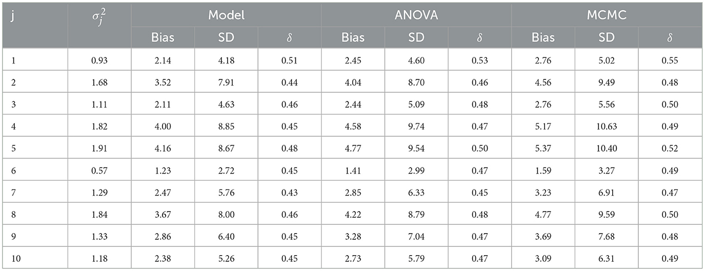
Table 1. Bias, SD, and δ for ${\sigma }_j^2$ with model, ANOVA, and MCMC methods.

For the cases j = 1, …, 10, our estimator consistently exhibited the smallest δ. The probability of this occurring by chance, assuming no superior precision among the methods, would be $q={(\frac{1}{3})}^{10}$. This provides strong evidence that our method demonstrates significantly greater precision.

6 Final remarks

In this paper, we consider biadditive models, often used in studies of manuring and other agronomic applications. We incorporated two extensions of these models: orthogonal block structures and commutative orthogonal block structures, which allow for a more detailed analysis of the additive structure of covariance matrices. In addition to individual models, we considered families of biadditive regression models. By incorporating commutative conditions, we derived optimal estimators, including best linear unbiased estimators and best quadratic unbiased estimators. The proposed methodology extends classical results, such as the Hsu theorem, while providing a robust framework for hypothesis testing within families of models. This framework also emphasizes the estimation of covariance components and coefficients, offering researchers valuable tools for investigating variability across models. The chi-square tests presented here establish a solid statistical foundation for evaluating variability and ensuring precision in agronomic studies. Furthermore, we highlighted the relevance of commutative orthogonal structures for factorial models, particularly those based on prime basis factorials. Such models, often used in studies of manuring and other agronomic applications, showcase the versatility of our approach. To evaluate the performance of the proposed methods, we conducted a simulation study. In this study, we simulated observation vectors based on biadditive regression models with predefined covariance structures and random effects. Using simulations conducted for our model, as well as for the ANOVA and MCMC methods, we estimated variance components and computed performance metrics, such as bias, SD, and δ. Simulation results demonstrated the enhanced precision of our estimation approach.

Data availability statement

The original contributions presented in the study are included in the article, further inquiries can be directed to the corresponding author.

Author contributions

MO: Investigation, Methodology, Writing – original draft, Writing – review & editing. EG: Investigation, Methodology, Writing – review & editing. AA: Writing – original draft, Writing – review & editing. JP: Writing – original draft, Writing – review & editing. JM: Methodology, Supervision, Conceptualization, Validation, Investigation, Writing – original draft, Writing – review & editing.

Funding

The author(s) declare that financial support was received for the research and/or publication of this article. MO was funded by projects UIDB/04674/2020 (CIMA) DOI: 10.54499/UIDB/04674/2020 and H2020-MSCA-RISE- 2020/101007950, with the title Decision Support for the Supply of Ecosystem Services under Global Change (DecisionES), funded by the Marie Curie International Staff Exchange Scheme. JP was funded by National funds through FCT – Fundação para a Ciência e a Tecnologia, I.P., under the projects UID/04209 and LA/P/0132/2020 (DOI: 10.54499/LA/P/0132/2020).

Conflict of interest

The authors declare that the research was conducted in the absence of any commercial or financial relationships that could be construed as a potential conflict of interest.

The author(s) declared that they were an editorial board member of Frontiers, at the time of submission. This had no impact on the peer review process and the final decision.

Publisher's note

All claims expressed in this article are solely those of the authors and do not necessarily represent those of their affiliated organizations, or those of the publisher, the editors and the reviewers. Any product that may be evaluated in this article, or claim that may be made by its manufacturer, is not guaranteed or endorsed by the publisher.

References

1. Pinheiro JC, Bates DM. Mixed-effects Models in S and S-PLUS. New York, NY: Springer (2000). doi: 10.1007/978-1-4419-0318-1

Crossref Full Text | Google Scholar

2. Demidenko E. Mixed Models: Theory and Applications With R. New York, NY: Wiley (2013).

Google Scholar

3. Sahai H, Ojeda MM. Analysis of variance for random models. In: Unbalanced data: Theory, methods, applications, and data analysis. Cambridge: Birkhäuser (2005). doi: 10.1007/978-0-8176-8168-5

Crossref Full Text | Google Scholar

4. Dempster AP, Selwyn MR, Patel CM, Roth AJ. Statistical and computational aspects of mixed model analysis. Appl Stat. (1984) 33:203–14. doi: 10.2307/2347446

Crossref Full Text | Google Scholar

5. Alexandre A, Oliveira M, Garção E, Mexia J. Biadditive models: commutativity and optimum estimators. Commun Stat. (2022) 53:2021–2033. doi: 10.1080/03610926.2022.2117560

Crossref Full Text | Google Scholar

6. Zmyslony R. A characterization of best linear unbiased estimators in the general linear model. J Mathem Stat Probab Theory. (1978) 2:365–78. doi: 10.1007/978-1-4615-7397-5_27

Crossref Full Text | Google Scholar

7. Kariya T, Kurata H. Generalized Least Squares. New York, NY: Wiley Series in Probability and Statistics (2004). doi: 10.1002/0470866993

Crossref Full Text | Google Scholar

8. Nelder JA. The analysis of randomized experiments with orthogonal block structure. I Block structure and the null analysis of variance. Proc R Soc Lond Ser A Math Phys Sci. (1965) 283:147–62. doi: 10.1098/rspa.1965.0012

Crossref Full Text | Google Scholar

9. Nelder JA. The analysis of randomized experiments with orthogonal block structure. II Treatment, structure and the general analysis of variance. Proc R Soc Lond Ser A Math Phys Sci. (1965) 283:163–78. doi: 10.1098/rspa.1965.0013

Crossref Full Text | Google Scholar

10. Caliński T, Kageyama S. Block Designs. A Randomization Approach. Volume I: analysis. Berlin: Springer (2000). doi: 10.1007/978-1-4612-1192-1

Crossref Full Text | Google Scholar

11. Caliński T, Kageyama S. A Randomization Approach. Volume II: design. Berlin: Springer (2003). doi: 10.1007/978-1-4419-9246-8

Crossref Full Text | Google Scholar

12. Shot JR. Matrix Analysis for Statistics 3rd ed. New York, NY: Wiley. (2017).

Google Scholar

13. Jordan P, Von Neumam J, Wingner G. An the algebra generation of quantum Mechanics formalism. J Ann Math. (1934) 1:25–64.

Google Scholar

14. Seely J. Quadratic subspaces and completeness. J Ann Math Stat. (1971) 42:710–21. doi: 10.1214/aoms/1177693420

Crossref Full Text | Google Scholar

15. Seely J, Zyskind G. Linear Spaces and summary variance unbiased estimations. J Ann Math Stat. (1971) 42:691–703. doi: 10.1214/aoms/1177693418

Crossref Full Text | Google Scholar

16. Hsu PL. On the best unbiased estimate of variance. Statist Res Mem. (1938) 2:91–104.

Google Scholar

17. Silvey SD. Statistical Inference. London: Chapman & Hall (1975).

Google Scholar

18. Scheffe H. The Analysis of Variance. New York, NY: Wiley (1959).

Google Scholar