A Riemann–Hilbert approach to solution of the modified focusing complex short pulse equation

We develop a Riemann–Hilbert approach to the modified focusing complex short pulse (mfcSP) equation

$u_{xt}=u+\frac{1}{2}\overline{u}{(u^2)}_{xx}$

with zero boundary conditions (as |x| → ∞). We obtain a parametric representation of the solution of the initial value problem for the mfcSP equation in terms of the solution of the associated Riemann–Hilbert problem. This representation is then used for retrieving one-soliton solutions.

1 Introduction

The short pulse equation (SP equation, or SPE)

$\begin{array}{ll}{u}_{xt}=u+\frac{1}{6}{(u^3)}_{xx}& (1)\end{array}$

was derived by Schäfer and Wayne [19] as a model equation for the propagation of ultra-short optical pulses in non-linear media. In this equation, u = u(x, t) is a real-valued function that represents the magnitude of the electric field. The short pulse equation is an alternative model to the non-linear Schrödinger (NLS) equation, the latter being used for describing the slow modulation of the amplitude of a weakly non-linear wave packet in a moving medium. NLS is used in non-linear optics with great success to describe slowly varying wave trains whose spectra are narrowly localized around the carrier frequency or to describe the propagation of sufficiently broad pulses. In the regime of ultra-short pulses where the width of optical pulse is in order of femtosecond, the SP equation is supposed to provide better approximation to the corresponding solution of the Maxwell equation while the NLS equation becomes less accurate. In [10], with the help of numerical simulations, it was shown that the SP equation can indeed be used to describe pulses with broad spectrum.

In [17, 18], it was shown that the SP equation is completely integrable, in the sense that it is the compatibility condition of a pair of linear, matrix-valued ordinary differential equations involving an external (spectral) parameter; such pair of equations is called the Lax pair. In the case of the SP equation, the associated Lax pair is as follows:

$\begin{array}{ll}{\Phi }_x=U\Phi ,& (2)\end{array}$

$\begin{array}{ll}{\Phi }_t=V\Phi ,& (3)\end{array}$

where U and V are 2 × 2 matrices dependent on the spectral parameter λ:

$\begin{array}{ll}U=\left(\begin{array}{cc}\lambda & \lambda u_x\\ \lambda u_x& -\lambda \end{array}\right),& (4)\end{array}$

$\begin{array}{ll}V=\left(\begin{array}{cc}\frac{\lambda }{2}{u}^2+\frac{1}{4\lambda }& \frac{\lambda }{2}{u}^2{u}_x-\frac{1}{2}u\\ \frac{\lambda }{2}{u}^2{u}_x+\frac{1}{2}u& -\frac{\lambda }{2}{u}^2-\frac{1}{4\lambda }\end{array}\right).& (5)\end{array}$

The Riemann–Hilbert approach to the study of solutions of the SP equation was presented in [8].

The modified short pulse (mSP) equation

$\begin{array}{ll}{u}_{xt}=u+\frac{1}{2}u{(u^2)}_{xx},& (6)\end{array}$

was proposed by Sakovich [16], who studied integrable non-linear equations having the form

$\begin{array}{ll}{u}_{xt}=u+a{u}^2{u}_{xx}+bu{u}_x^2.& (7)\end{array}$

When $\frac{a}{b}=\frac{1}{2}$, Equation 7 reduces to Equation 1 whereas the case $\frac{a}{b}=1$ reduces to Equation 6, both cases being integrable. The mSP equation (6) was studied by Guo and Liu, who constructed soliton solutions by the Riemann–Hilbert method [14]. Matsuno [15] proposed the N- component generalization of Equation 6, which in the case N = 2 reads

$\begin{array}{ll}{u}_{xt}=u+\frac{1}{2}v{(u^2)}_{xx},v_{xt}=v+\frac{1}{2}u{(v^2)}_{xx}.& (8)\end{array}$

Matsuno constructed the soliton solutions by solving the associated bilinear equations and constructed the local and non-local conservation laws of Equation 8.

Obviously, if v = u, then Equation 8 reduces to Equation 6. On the other hand, if v = ū, where the bar stands for the complex conjugation, the system (8) reduces [20] to

$\begin{array}{ll}{u}_{xt}=u+\frac{1}{2}\overline{u}{(u^2)}_{xx},& (9)\end{array}$

which will be called in what follows the modified focusing complex short pulse equation (mfcSP equation or mfcSPE). Notice that the reduction v = −ū gives rise to a defocusing version of Equation 9, having the minus sign at the place of the plus. In [20], some multiple smooth soliton, cuspon soliton, loop soliton, breather, and rogue wave solutions are constructed by N-fold Darboux transformation.

From the point of view of possible applications in optics, the mfcSP equation, being formulated for a complex-valued function, appears to be more informative: Similarly to the NLS equation, a complex-valued function can contain not only the information about the amplitude but also about the phase of the associated electromagnetic wave. On the other hand, the mfcSP equation is integrable: Its Lax pair is Equation 2, where [20]

$\begin{array}{ll}U=\lambda \left(\begin{array}{cc}1-u_x{\overline{u}}_x& 2u_x\\ 2{\overline{u}}_x& -1+u_x{\overline{u}}_x\end{array}\right),& (10)\end{array}$

$\begin{array}{ll}V=\left(\begin{array}{cc}\frac{1}{4\lambda }+\lambda (1-u_x{\overline{u}}_x)|u{|}^2& -u+2\lambda |u{|}^2{u}_x\\ \overline{u}+2\lambda |u{|}^2{\overline{u}}_x& -\frac{1}{4\lambda }-\lambda (1-u_x{\overline{u}}_x)|u{|}^2\end{array}\right).& (11)\end{array}$

Motivated by the above, in the present study, we develop a Riemann–Hilbert (RH) problem formalism for the inverse scattering transform to the initial value problem for the mfcSPE:

$\begin{array}{ll}{u}_{xt}=u+\frac{1}{2}\overline{u}{(u^2)}_{xx},t>0,-\infty <x<+\infty ,& (12)\end{array}$

$\begin{array}{ll}u(x,0)=u_0(x),-\infty <x<+\infty .& (13)\end{array}$

We assume that u₀(x) decays sufficiently fast at ±∞:

$u_0(x)\to 0,x\to \pm \infty ,$

and we seek a solution u(x, t) that decays as x → ±∞ for all t > 0:

$u(x,t)\to 0,x\to \pm \infty .$

Notice that the RH approach for solving initial value problems for integrable non-linear PDE can be viewed as a version of the inverse scattering transform (IST) method for such problems, the more traditional realization of which is based on deriving and solving the Marchenko integral equation for the corresponding inverse problems, see, for example, [1] and references therein. Since the latter approach requires the representation of special solutions of the x-equation of the corresponding Lax pair in terms of so-called transformation operators, its application to cases where the dependence of the Lax equations on the spectral parameter is more involved (comparing, for example, with the case of the Korteweg-de Vries equation and its modified versions) is not straightforward because the very existence of the corresponding transformation operators is questionable. On the other hand, as we will show in the next section, the formalism of the RH problem allows us to establish an algorithmic procedure providing special solutions of the Lax pair equations with the necessary analytic properties.

In Section 2, we present a version of the Lax pair associated with the mfcSP equation, which is more convenient for controlling analytical properties of its special solutions, also known as the Jost solutions. They are then used in Section 3 to formulate a matrix Riemann–Hilbert problem suitable for solving the Cauchy problem (12). In this way, we give a representation of the solution u(x, t) of the problem (12) in terms of the solution of this RH problem. Then, in Section 4, we show that a solution of the RH problem with any appropriate jump matrix (ensuring the unique solvability of the RH problem) gives rise to a solution of the mfcSPE. In Section 5, we discuss the construction of soliton solutions using the formalism of the RH problem, which is illustrated numerically in Section 6.

2 Lax pairs and eigenfunctions

The RH formalism for integrable non-linear equations utilizes the possibility of constructing special solutions of linear equations from the associated Lax pair, which are well controlled as functions of the spectral parameter, in the whole extended complex plane. For this purpose, it is useful to have the Lax pair equations in the form suitable for establishing analytic properties of solutions near the singular points with respect to spectral parameter of the Lax pair equations. For different domains in the complex plane, these solutions are defined differently and are related to each other at the boundaries between these domains.

To construct such special solutions of the differential equations from the Lax pair, it is convenient to pass to integral equations, whose solutions are particular solutions to the Lax pair equation.

Notice the coefficients U and V of the Lax pair are traceless matrices. Consequently, the determinant of a matrix solution to Equation 10 (composed of two vector solutions) is independent of x and t.

To obtain a RH problem with the jump condition on the real axis, as in the case of other Camassa–Holm-type equations [see [3–9]], we redefine the spectral parameter introducing k: = iλ.

Notice that U and V have singularities (in the extended complex k-plane) at k = 0 and at k = ∞. Namely, since U is singular at k = ∞ only, for dealing with the problem on the whole x-line it is important to control the behavior of special solutions of the Lax pair equations for large k. Assume that u(·, t) ∈ W^{2, 1}(ℝ) and transform the Lax pair to the following form [cf. [2–4, 8]]:

$\begin{array}{ll}{\widehat{\Phi }}_x+Q_x\widehat{\Phi }=\widehat{U}\widehat{\Phi },& (14)\end{array}$

$\begin{array}{ll}{\widehat{\Phi }}_t+Q_t\widehat{\Phi }=\widehat{V}\widehat{\Phi },& (15)\end{array}$

where the coefficients Q(x, t, k), Û(x, t, k), and $\widehat{V}(x,t,k)$ have the following properties:

1. Q is diagonal and is unbounded as k → ∞.

2. Û = O(1) and $\widehat{V}=\text{O}(1)$ as k → ∞.

3. The diagonal parts of Û and $\widehat{V}$ decay as k → ∞.

4. Û → 0 and $\widehat{V}\to 0$ as x → ±∞.

To transform the Lax pair, we introduce $\widehat{\Phi }:=G\Phi$ with G = G(x, t) to be defined. Then, the Lax pair (10) takes form

$\begin{array}{ll}{\widehat{\Phi }}_x=GU{G}^{-1}\widehat{\Phi }+G_x{G}^{-1}\widehat{\Phi },& (16)\end{array}$

$\begin{array}{ll}{\widehat{\Phi }}_t=GV{G}^{-1}\widehat{\Phi }+G_t{G}^{-1}\widehat{\Phi }.& (17)\end{array}$

Since U is a product of the spectral parameter and a matrix independent of it, we can define G so as $Q_x:=-GU{G}^{-1}$ is a diagonal matrix function satisfying item (i). Then, the degree of freedom in the determination of G (multiplication of G by a diagonal matrix from the left) can be used to provide us with Û satisfying (iii). Namely, introducing

$\begin{array}{ll}q(x,t):=1+|u_x(x,t){|}^2& (18)\end{array}$

we have

$\begin{array}{ll}G(x,t)=\frac{1}{\sqrt{q}}\left(\begin{array}{cc}{e}^{-m}& e^{-m}{u}_x\\ -e^m{\overline{u}}_x& e^m\end{array}\right)& (19)\end{array}$

with the inverse

$\begin{array}{ll}{G}^{-1}(x,t)=\frac{1}{\sqrt{q}}\left(\begin{array}{cc}{e}^m& -e^{-m}{u}_x\\ e^m{\overline{u}}_x& e^{-m}\end{array}\right),& (20)\end{array}$

where m is not specified for the moment. Then,

$\begin{array}{ll}{Q}_x(x,t,k)=-GU{G}^{-1}=\text{i}kq(x,t)\left(\begin{array}{cc}1& 0\\ 0& -1\end{array}\right)=\text{i}kq(x,t){\sigma }_3,& (21)\end{array}$

where σ₃ is the Pauli matrix ${\sigma }_3=\left(\begin{array}{cc}1& 0\\ 0& -1\end{array}\right)$.

To satisfy item (iii) for Û, we use the freedom of choice of m to make the diagonal part of $\widehat{U}=G_x{G}^{-1}$ to be identically equal to zero. Complemented by a norming condition m(+∞, t) = 0, this leads to

$\begin{array}{ll}m(x,t):=\frac{1}{2}{\displaystyle {\int }_x^{\infty }}\frac{u_z{\overline{u}}_{zz}-u_{zz}{\overline{u}}_z}{1+|u_z{|}^2}(z,t)\text{d}z,& (22)\end{array}$

which finally gives

$\begin{array}{ll}\widehat{U}=\widehat{U}(x,t)=\frac{1}{q}\left(\begin{array}{cc}0& e^{-2m}{u}_{xx}\\ -e^{2m}{\overline{u}}_{xx}& 0\end{array}\right).& (23)\end{array}$

Notice that m is purely imaginary and thus $\bar{m}=-m$ and |e^m| = 1.

As for the t–equation (17), we have:

$\begin{array}{l}GV{G}^{-1}+G_t{G}^{-1}=(-\text{i}kq{\left|u\right|}^2-\frac{1}{4\text{i}kq}(1-u_x{\overline{u}}_x)-m_t+\\ \frac{1}{2q}({\overline{u}}_x(-2u+u_{xt})+u_x(2\overline{u}-{\overline{u}}_{xt}))){\sigma }_3\\ +\frac{1}{2\text{i}kq}\left(\begin{array}{cc}0& {\text{e}}^{-2m}{u}_x\\ {\text{e}}^{2m}{\overline{u}}_x& 0\end{array}\right)\\ +\frac{1}{q}\left(\begin{array}{cc}0& -{\text{e}}^{-2m}(\overline{u}{u}_x^2+u-u_{xt})\\ {\text{e}}^{2m}(u{\overline{u}}_x^2+\overline{u}-{\overline{u}}_{xt})& 0\end{array}\right).& (24)\end{array}$

Now, we can determine Q(x, t, k) by integrating Equation 21 w.r.t. x and taking into account that we want $\widehat{V}$ in Equation 15 to vanish at x = ±∞ for all t. This gives

$\begin{array}{ll}Q(x,t,k):=\left(\text{i}k\widehat{x}(x,t)+\frac{t}{4\text{i}k}\right){\sigma }_3,& (25)\end{array}$

where

$\begin{array}{ll}\widehat{x}(x,t):=x-{\displaystyle {\int }_x^{\infty }}(q(y,t)-1)\text{d}y& (26)\end{array}$

is normalized in such a way that $\widehat{x}-x\to 0$ as x → +∞. Then, we have

$Q_t(x,t,k)=\left(\text{i}k{\widehat{x}}_t(x,t)+\frac{1}{4\text{i}k}\right){\sigma }_3=\left(\text{i}k|u{|}^{2}q(x,t)+\frac{1}{4\text{i}k}\right){\sigma }_3,$

where we have used the equality $q_t={(|u{|}^{2}q)}_x$ which is actually the mfcSPE (9) rewritten as a conservation law. Correspondingly,

$\begin{array}{l}\widehat{V}(x,t,k)=\left(\frac{|u_x{|}^2}{2\text{i}kq}-m_t+\frac{1}{2q}({\overline{u}}_x(-2u+u_{xt})+u_x(2\overline{u}-{\overline{u}}_{xt}))\right){\sigma }_3\\ +\frac{1}{2\text{i}kq}\left(\begin{array}{cc}0& e^{-2m}{u}_x\\ e^{2m}{\overline{u}}_x& 0\end{array}\right)\\ +\frac{1}{q}\left(\begin{array}{cc}0& -{\text{e}}^{-2m}(\overline{u}{u}_x^2+u-u_{xt})\\ e^{2m}(u{\overline{u}}_x^2+\overline{u}-{\overline{u}}_{xt})& 0\end{array}\right).& (27)\end{array}$

Remark 2.1. The dependence of the diagonal matrix Q on variables $\widehat{x}$ and t, see Equation 25, is the same as in the case of the SP equation [see [8]]. This justifies the name of the mfcSPE as the modified SP equation: The same property holds for the pair consisting of the famous Korteweg–de Vries equation u_t + 6uu_x + u_xxx = 0 and the modified Korteweg–de Vries equation $u_t+6u^2{u}_x+u_{xxx}=0$.

Introducing

$\begin{array}{ll}\tilde{\Phi }=\widehat{\Phi }{\text{e}}^Q,& (28)\end{array}$

Equations 14 can be rewritten as

$\begin{array}{ll}{\tilde{\Phi }}_x+\left[Q_x,\tilde{\Phi }\right]=\widehat{U}\tilde{\Phi },& (29)\end{array}$

$\begin{array}{ll}{\tilde{\Phi }}_t+\left[Q_t,\tilde{\Phi }\right]=\widehat{V}\tilde{\Phi },& (30)\end{array}$

where [·, ·] denotes the matrix commutator. Now, we determine the special (Jost) solutions ${\tilde{\Phi }}_{\pm }(x,t,k)$ of Equation 29 as the 2 × 2 matrix-valued solutions of the associated Volterra integral equations:

$\begin{array}{ll}{\tilde{\Phi }}_{\pm }(x,t,k)=I+{\displaystyle {\int }_{\pm \infty }^x}{\text{e}}^{Q(y,t,k)-Q(x,t,k)}\widehat{U}(y,t){\tilde{\Phi }}_{\pm }(y,t,k){\text{e}}^{Q(x,t,k)-Q(y,t,k)}\text{d}y,& (31)\end{array}$

where I is the identity matrix. Taking into account the definition of Q (25) and (26), we get

$\begin{array}{ll}{\tilde{\Phi }}_{+}(x,t,k)=I-{\displaystyle {\int }_x^{\infty }}{\text{e}}^{\text{i}k{\displaystyle {\int }_x^y}q(\xi ,t)\text{d}\xi {\sigma }_3}\widehat{U}(y,t){\tilde{\Phi }}_{+}(y,t,k){\text{e}}^{-\text{i}k{\displaystyle {\int }_x^y}q(\xi ,t)\text{d}\xi {\sigma }_3}\text{d}y,& (32)\end{array}$

$\begin{array}{ll}{\tilde{\Phi }}_{-}(x,t,k)=I+{\displaystyle {\int }_{-\infty }^x}{\text{e}}^{-\text{i}k{\displaystyle {\int }_y^x}q(\xi ,t)\text{d}\xi {\sigma }_3}\widehat{U}(y,t){\tilde{\Phi }}_{-}(y,t,k){\text{e}}^{\text{i}k{\displaystyle {\int }_y^x}q(\xi ,t)\text{d}\xi {\sigma }_3}\text{d}y.& (33)\end{array}$

Respectively, ${\widehat{\Phi }}_{\pm }:={\tilde{\Phi }}_{\pm }{e}^{-Q}$ are the Jost solutions of the Lax pair equations (14).

In what follows, the columns of a 2 × 2 matrix $\mu =(\begin{array}{cc}{\mu }^{(1)}& {\mu }^{(2)}\end{array})$ are denoted by μ⁽¹⁾ and μ⁽²⁾. Since q is positive, the exponentials in Equation 32 as functions of y either decay to 0 or grow to ∞ as y goes to +∞ or to −∞, depending on the sign of the imaginary part of k (for real k, all exponentials are oscillating functions). Moreover, if we consider Equation 32 columnwise, the corresponding integral equation involves the exponentials of only one sign: either ${\text{e}}^{\text{i}k{\int }_x^{y}q(\xi ,t)\text{d}\xi }$ or ${\text{e}}^{-\text{i}k{\int }_x^{y}q(\xi ,t)\text{d}\xi }$. Consequently, we can determine the columns of Equation 32 via Neumann series for the corresponding integral equation, which converge if k belongs to the corresponding half–plane: the upper half–plane {k|Imk ≥ 0} or the lower half–plane {k|Imk ≤ 0}. The obtained Jost solutions satisfy the following properties [cf. [8]] for all (x, t):

1. $det{\tilde{\Phi }}_{\pm }\equiv 1$ (the consequence of the traceless of the coefficient matrices in Equation 14.

2. ${\tilde{\Phi }}_{-}^{(1)}$ and ${\tilde{\Phi }}_{+}^{(2)}$ are analytic in {k∣Imk > 0} and continuous in {k∣Imk ≥ 0, k ≠ 0}.

3. ${\tilde{\Phi }}_{+}^{(1)}$ and ${\tilde{\Phi }}_{-}^{(2)}$ are analytic in {k∣Imk < 0} and continuous in {k∣Imk ≤ 0, k ≠ 0}.

4. $(\begin{array}{cc}{\tilde{\Phi }}_{-}^{(1)}& {\tilde{\Phi }}_{+}^{(2)}\end{array})\to I$ as k → ∞ in {k∣Imk ≥ 0}.

5. $(\begin{array}{cc}{\tilde{\Phi }}_{+}^{(1)}& {\tilde{\Phi }}_{-}^{(2)}\end{array})\to I$ as k → ∞ in {k∣Imk ≤ 0}.

6. Symmetry property:

$\begin{array}{ll}\overline{{\tilde{\Phi }}_{\pm }(·,·,\bar{k})}=\left(\begin{array}{cc}0& 1\\ -1& 0\end{array}\right){\tilde{\Phi }}_{\pm }(·,·,k)\left(\begin{array}{cc}0& -1\\ 1& 0\end{array}\right).& (34)\end{array}$

The last property is due to the symmetry of the matrix Ǔ: = Û−ikqσ₃:

$\begin{array}{ll}\overline{\check{U}(·,·,\bar{k})}=\left(\begin{array}{cc}0& 1\\ -1& 0\end{array}\right)\check{U}(·,·,k)\left(\begin{array}{cc}0& -1\\ 1& 0\end{array}\right).& (35)\end{array}$

Remark 2.2. Introducing the new variable $\widehat{x}$ as in Equation 26, Equation 14 reduces to the (non-self-adjoint) Dirac equation for $\stackrel{⌣}{\Phi }(\widehat{x},t,k):=\widehat{\Phi }(x(\widehat{x},t),t,k)$:

$\begin{array}{ll}{\stackrel{⌣}{\Phi }}_{\widehat{x}}+\text{i}k{\sigma }_3\stackrel{⌣}{\Phi }=\stackrel{⌣}{U}\stackrel{⌣}{\Phi },& (36)\end{array}$

where

$\begin{array}{ll}\stackrel{⌣}{U}=\frac{1}{q}\left(\begin{array}{cc}0& {\text{e}}^{-2m}{u}_{xx}\\ -{\text{e}}^{2m}{\overline{u}}_{xx}& 0\end{array}\right).& (37)\end{array}$

Equation 36 is the spatial equation from the Lax pair associated with the focusing non-linear Schrödinger (fNLS) equation, see [12]. Therefore, the analytic properties of ${\tilde{\Phi }}_{\pm }$ stated above are the same as in the case of the fNLS equation considered in [12].

Now, we introduce the scattering matrix s(k) as the matrix relating the Jost solutions ${\widehat{\Phi }}_{+}$ and ${\widehat{\Phi }}_{-}$ for those values of k where all their columns are determined (i.e., for real k):

$\begin{array}{ll}{\widehat{\Phi }}_{+}(\widehat{x},t,k)={\widehat{\Phi }}_{-}(\widehat{x},t,k)s(k),k\in ℝ& (38)\end{array}$

or, in terms of ${\tilde{\Phi }}_{\pm }$,

$\begin{array}{ll}{\tilde{\Phi }}_{+}(\widehat{x},t,k)={\tilde{\Phi }}_{-}(\widehat{x},t,k){\text{e}}^{-Q(\widehat{x},t,k)}s(k){\text{e}}^{Q(\widehat{x},t,k)},k\in ℝ.& (39)\end{array}$

Notice that since ${\widehat{\Phi }}_{+}$ and ${\widehat{\Phi }}_{-}$ are solutions of the same differential equations (16), the matrix s(k) does not depend on $\widehat{x}$ and t. Consequently, s(k) can be determined by q(x, 0) only, by

$s(k)={\tilde{\Phi }}_{-}^{-1}(0,0,k){\tilde{\Phi }}_{+}(0,0,k).$

Indeed, ${\tilde{\Phi }}_{\pm }(\widehat{x},0,k)$ are determined [see Equation 32] by Û(x, 0) and q(x, 0) which, in turn, are determined by q(x, 0) alone.

Due to the symmetry (34) and the fact that e^{Q(x, t, k)} satisfies the same symmetry as well, the scattering matrix can be rewritten with the help of two scalar spectral functions, a(k) and b(k), as follows:

$\begin{array}{ll}s(k)=\left(\begin{array}{cc}\overline{a(k)}& b(k)\\ -\overline{b(k)}& a(k)\end{array}\right),k\in ℝ.& (40)\end{array}$

Taking into account Remark 2.2, the spectral functions have properties, which are similar to those in case of the fNLS equation in [12]:

1. a(k) and b(k) are determined by u(x, 0) through the solutions ${\tilde{\Phi }}_{\pm }(x,0)$ of Equation 32, where Û = Û(x, 0) is defined by Equation 23 with u replaced by u₀(x) (same for q).

2. a(k) is analytic in {k|Imk > 0} and continuous in {k|Imk ≥ 0}, moreover, a(k) → 1 as k → ∞.

3. b(k) is continuous for k ∈ ℝ and b(k) → 0 as |k| → ∞.

4. |a(k)|² + |b(k)|² = 1 for k ∈ ℝ.

5. Let ${\left\{k_j\right\}}_1^N$ be the set of zeros of a(k) in {k|Imk > 0}. We will make the genericity assumption that the amount of these zeros is finite and there are no real zeros. Then, ${\widehat{\Phi }}_{-}^{(1)}(x,t,k_j)$ and ${\widehat{\Phi }}_{+}^{(2)}(x,t,k_j)$ are linearly dependent solutions of Equation 14 and thus

$\begin{array}{ll}{\tilde{\Phi }}_{-}^{(1)}(x,t,k_j)={\text{e}}^{2\text{i}{k}_j\widehat{x}(x,t)+\frac{t}{2\text{i}{k}_j}}{\tilde{\Phi }}_{+}^{(2)}(x,t,k_j){\alpha }_j& (41)\end{array}$

with the constants α_j, which, similarly to r(k) are determined by u₀(x) setting t = 0 in Equation 41.

3 The Riemann–Hilbert problem

3.1 A RH problem constructed from special eigenfunctions

In this section, we consider the generic situation when all zeros of a(k) in {k|Imk > 0} are simple. Then, the analytic properties of ${\tilde{\Phi }}_{\pm }$ stated above allow us to rewrite the scattering relations in Equation 39 as a jump relation for a meromorphic (w.r.t. k), 2 × 2 matrix–valued function (depending on x and t as parameters). Define M(x, t, k) as follows (where the scalar factors are introduced in order to provide det M ≡ 1):

$\begin{array}{ll}M(x,t,k)=\{\begin{array}{cc}\left(\begin{array}{cc}\frac{{\tilde{\Phi }}_{-}^{(1)}(x,t,k)}{a(k)}& {\tilde{\Phi }}_{+}^{(2)}(x,t,k)\end{array}\right),& Imk>0,\\ \left(\begin{array}{cc}{\tilde{\Phi }}_{+}^{(1)}(x,t,k)& \frac{{\tilde{\Phi }}_{-}^{(2)}(x,t,k)}{\overline{a(\overline{k})}}\end{array}\right),& Imk<0.\end{array}& (42)\end{array}$

Define also the reflection coefficient:

$\begin{array}{ll}r(k):=\frac{\overline{b(k)}}{a(k)},k\in ℝ.& (43)\end{array}$

Then, the limiting values of M as k approaches the real axis from the domains ±Imk > 0 (we denote them by M_±(x, t, k), k ∈ ℝ) are related as follows:

$\begin{array}{ll}{M}_{+}(x,t,k)=M_{-}(x,t,k){\text{e}}^{-Q(x,t,k)}{J}_0(k){\text{e}}^{Q(x,t,k)},k\in ℝ,& (44)\end{array}$

where

$\begin{array}{ll}{J}_0(k)=\left(\begin{array}{cc}1+|r(k){|}^2& \overline{r(k)}\\ r(k)& 1\end{array}\right).& (45)\end{array}$

Taking into account the properties of ${\tilde{\Phi }}_{\pm }$ and s(k), the function M(x, t, k) satisfies the following properties:

1. det M ≡ 1.

2. Normalization: M(·, ·, k) → I as k → ∞.

3. Symmetry:

$\begin{array}{ll}\overline{M(·,·,\overline{k})}=\left(\begin{array}{cc}0& 1\\ -1& 0\end{array}\right)M(·,·,k)\left(\begin{array}{cc}0& -1\\ 1& 0\end{array}\right).& (46)\end{array}$

4. M⁽¹⁾ has poles at the zeroes k_j, j = 1, 2, …, N, of a(k) (in the upper half-plane), M⁽²⁾ has poles at $\overline{k_j}$ (in the lower half-plane), and the following conditions are satisfied:

$\begin{array}{ll}{Res}_{k=k_j}{M}^{(1)}(x,t,k)=\text{i}{\alpha }_j{\text{e}}^{2\text{i}{k}_{j}x(\widehat{x},t)+\frac{t}{2\text{i}{k}_j}}{M}^{(2)}(x,t,k_j),& (47)\end{array}$

$\begin{array}{ll}{Res}_{k=\overline{k_j}}{M}^{(2)}(x,t,k)=\text{i}\overline{{\alpha }_j}{\text{e}}^{-2\text{i}\overline{k_j}x(\widehat{x},t)-\frac{t}{2\text{i}\overline{k_j}}}{M}^{(1)}(x,t,\overline{k_j})& (48)\end{array}$

where α_j, j = 1, 2, …, N, are constants.

The idea of the Riemann-Hilbert approach in the inverse scattering method consists of considering the jump relation in Equation 44 complemented by the normalization condition M → I as k → ∞ and by the residue conditions (47) as the problem of finding M(x, t, k) given the jump condition (44) (with a given jump matrix) and the residue conditions (47) [i.e., given (k_j, α_j), j = 1, ..., N] at the singularities of M.

As in the case of other Camassa–Holm-type equations [particularly, the SPE, see [8]], one faces the problem that the determination of the jump matrix $({\text{e}}^{-Q(x,t,k)}{J}_0(k){\text{e}}^{Q(x,t,k)})$ involves not only the objects that are uniquely determined by the initial data u(x, 0) [i.e., the spectral functions a(k) and b(k) involved in J₀(k)] but also Q(x, t, k), which is not determined by u(x, 0): Its definition involves u(x, t) for t > 0.

We can resolve this problem by considering a RH problem depending, instead of (x, t), on the parameters $\widehat{x}$ and t; in this way, the jump and residue data become explicit (in terms of $\widehat{x}$ and t). Actually, we introduce

$\begin{array}{ll}\widehat{M}(\widehat{x},t,k):=M(x(\widehat{x},t),t,k).& (49)\end{array}$

In terms of $\widehat{M}(\widehat{x},t,k)$, the jump condition takes the form:

$\begin{array}{ll}{\widehat{M}}_{+}(\widehat{x},t,k)={\widehat{M}}_{-}(\widehat{x},t,k)J(\widehat{x},t,k),k\in ℝ,& (50)\end{array}$

where

$\begin{array}{ll}J(\widehat{x},t,k):={\text{e}}^{-\widehat{Q}(\widehat{x},t,k)}{J}_0(k){\text{e}}^{\widehat{Q}(\widehat{x},t,k)}& (51)\end{array}$

with J₀ defined by Equation 45 and

$\begin{array}{ll}\widehat{Q}(\widehat{x},t,k)=\left(\text{i}k\widehat{x}+\frac{t}{4\text{i}k}\right){\sigma }_3& (52)\end{array}$

[so that $\widehat{Q}(\widehat{x},t,k)=Q(x(\widehat{x},t),t,k)$].

The residue conditions (47) also involve $\widehat{x}$ and t explicitly:

$\begin{array}{ll}{Res}_{k=k_j}{\widehat{M}}^{(1)}(\widehat{x},t,k)=\text{i}{\alpha }_j{\text{e}}^{2\text{i}{k}_j\widehat{x}+\frac{t}{2\text{i}{k}_j}}{\widehat{M}}^{(2)}(\widehat{x},t,k_j),& (53)\end{array}$

$\begin{array}{ll}{Res}_{k=\overline{k_j}}{\widehat{M}}^{(2)}(\widehat{x},t,k)=\text{i}\overline{{\alpha }_j}{\text{e}}^{-2\text{i}\overline{k_j}\widehat{x}-\frac{t}{2\text{i}\overline{k_j}}}{\widehat{M}}^{(1)}(\widehat{x},t,\overline{k_j})& (54)\end{array}$

On the one hand, the jump and residue conditions above were obtained assuming that there exists a solution u(x, t) of the mfcSP equation which decays as x → ±∞ for any t > 0. On the other hand, conditions (45), (50)–(53) can be considered as a factorization problem of the Riemann–Hilbert type, whose data are completely determined by u(x, 0).

RH problem. Given $\left\{r(k),k\in ℝ;{(k_j,{\alpha }_j)}_1^N\right\}$, find a piece-wise (w.r.t to ℝ) meromorphic function $\widehat{M}(\widehat{x},t,k)$ that satisfies conditions (45), (50)–(53) and the normalization condition:

$\begin{array}{ll}\widehat{M}(\widehat{x},t,k)\to I\text{ as }k\to \infty .& (55)\end{array}$

3.2 RH problem with second-order poles

In this section, to get more examples of “explicit” solutions to the mfcSPE, see Section 6 below, we allow the scattering function a(k) to have second-order zeroes in the upper half-plane, meaning that $\widehat{M}(\widehat{x},t,k)$ has second-order poles. We develop the generalization of the residue conditions on the columns of $\widehat{M}$ at the poles, which provides the unique solvability of the respective RH problem. These conditions include more relations between the coefficients of the Laurent expansions of the columns of $\widehat{M}(\widehat{x},t,k)$.

Let ${\left\{k_j\right\}}_1^N$ be the set of second–order zeroes of a(k). Consider the Laurent expansion of $\widehat{M}(\widehat{x},t,k)$ defined by Equation 42 and the expansion of a(k) as k → k_j:

$\begin{array}{ll}{\widehat{M}}^{(1)}(k)=\frac{{\widehat{M}}_{-2}^{(1)}}{{(k-k_j)}^2}+\frac{{\widehat{M}}_{-1}^{(1)}}{(k-k_j)}+{\widehat{M}}_0^1+\text{O}(k-k_j),& (56)\end{array}$

$\begin{array}{ll}{\widehat{M}}^{(2)}(k)={\widehat{M}}_0^{(2)}+{\widehat{M}}_1^{(2)}(k-k_j)+{\widehat{M}}_1^{(2)}{(k-k_j)}^2+\text{O}{(k-k_j)}^3,& (57)\end{array}$

$\begin{array}{ll}a(k)=a_2{(k-k_j)}^2+a_3{(k-k_j)}^3+\text{O}{(k-k_j)}^4.& (58)\end{array}$

The definition of the scattering matrix (38) provides us with the equality

$a(k)=det({\widehat{\Phi }}_{-}^{(1)}(\widehat{x},t,k){\widehat{\Phi }}_{+}^{(2)}(\widehat{x},t,k)).$

Since k_j is a zero of a(k), the columns ${\widehat{\Phi }}_{-}^{(1)}$ and ${\widehat{\Phi }}_{+}^2$ are linearly dependent; in terms of $\tilde{\Phi }$, this reads:

$\begin{array}{ll}{\tilde{\Phi }}_{+}^{(2)}(\widehat{x},t,k_j){\text{e}}^{2\text{i}{k}_j\widehat{x}+\frac{t}{2\text{i}{k}_j}}={\tilde{\Phi }}_{-}^{(1)}(\widehat{x},t,k_j)c_j& (59)\end{array}$

with some constant c_j.

Passing to the limit k → k_j for ${\widehat{M}}^{(1)}(k){(k-k_j)}^2$, where $\widehat{M}$ is defined by Equation 42, and using Equation 59 we get our first singularity condition:

$\begin{array}{ll}{\widehat{M}}_{-2}^{(1)}(\widehat{x},t)=\frac{1}{a_2{c}_j}{\text{e}}^{2\text{i}{k}_j\widehat{x}+\frac{t}{2\text{i}{k}_j}}{\widehat{M}}_0^{(2)}(\widehat{x},t).& (60)\end{array}$

Next, we consider the derivative of a(k). Taking into account the linear dependence of ${\widehat{\Phi }}_{-}^{(1)}(k_j)$ and ${\widehat{\Phi }}_{+}^{(2)}(k_j)$, we have

$ȧ(k_j)=det\left({\stackrel{.}{\widehat{\Phi }}}_{-}^{(1)}(k_j)-\frac{1}{c_j}{\stackrel{.}{\widehat{\Phi }}}_{+}^{(2)}(k_j){\widehat{\Phi }}_{+}^{(2)}(k_j)\right)=0,$

where the dot denotes the derivative w.r.t. k. Thus, we can introduce $d_j(\widehat{x},t)$ such that

$\begin{array}{ll}{\dot{\widehat{\Phi }}}_{-}^{(1)}(\widehat{x},t,k_j)-\frac{1}{c_j}{\dot{\widehat{\Phi }}}_{+}^{(2)}(\widehat{x},t,k_j)=d_j(\widehat{x},t){\widehat{\Phi }}_{+}^{(2)}(\widehat{x},t,k_j).& (61)\end{array}$

Unlike c_j, it is not clear immediately that d_j is independent of $\widehat{x}$ and t. To check this out, we differentiate Equation 61 w.r.t. $\widehat{x}$ and consider the matrix entries 11 and 12:

$\begin{array}{ll}{({\dot{\widehat{\Phi }}}_{-}^{11})}_{\widehat{x}}-\frac{1}{c_j}{({\dot{\widehat{\Phi }}}_{+}^{12})}_{\widehat{x}}={(d_j)}_{\widehat{x}}{\widehat{\Phi }}_{+}^{12}+d_j{({\dot{\widehat{\Phi }}}_{+}^{12})}_{\widehat{x}}.& (62)\end{array}$

Rewriting the Lax pair equations (14) in the form

${\widehat{\Phi }}_{\widehat{x}}=\check{U}\widehat{\Phi },{\widehat{\Phi }}_t=\check{V}\widehat{\Phi }$

and also differentiating them w.r.t. k, Equation 62 can be written as

$\begin{array}{l}{\stackrel{\dot{ˇ}}{U}}^{11}{\widehat{\Phi }}_{-}^{11}+{\stackrel{\dot{ˇ}}{U}}^{12}{\widehat{\Phi }}_{-}^{21}+{\check{U}}^{11}{\dot{\widehat{\Phi }}}_{-}^{11}+\\ {\check{U}}^{12}{\dot{\widehat{\Phi }}}_{-}^{21}-\frac{1}{c_j}({\stackrel{\dot{ˇ}}{U}}^{11}{\widehat{\Phi }}_{+}^{12}+\\ {\stackrel{\dot{ˇ}}{U}}^{12}{\widehat{\Phi }}_{+}^{22}+{\check{U}}^{11}{\dot{\widehat{\Phi }}}_{+}^{12}+{\check{U}}^{12}{\dot{\widehat{\Phi }}}_{+}^{22})\\ ={(d_j)}_{\widehat{x}}{\widehat{\Phi }}_{+}^{12}+d_j({\check{U}}^{11}{\widehat{\Phi }}_{+}^{12}+{\check{U}}^{12}{\widehat{\Phi }}_{+}^{22}).& (63)\end{array}$

Now, using the linear dependence of ${\widehat{\Phi }}_{-}^{(1)}$ and ${\widehat{\Phi }}_{+}^2$ and Equation 61, the respective terms in Equation 63 cancel out, thus leaving us with ${(d_j)}_{\widehat{x}}=0$. Since these computations are not specific for the derivative w.r.t. $\widehat{x}$, we can deduce (_dj)t = 0 as well and thus $d_j(\widehat{x},t)=d_j$ is independent of $\widehat{x}$ and t.

In terms of $\tilde{\Phi }$, equality (61) reads

$\begin{array}{c}{\dot{\tilde{\Phi }}}_{-}^{(1)}(\widehat{x},t,k_j)-\frac{1}{c_j}{\text{e}}^{2\text{i}{k}_j\widehat{x}+\frac{t}{2\text{i}{k}_j}}{\dot{\tilde{\Phi }}}_{+}^{(2)}(\widehat{x},t,k_j)=\left(d_j+\frac{2(\text{i}\widehat{x}-\frac{t}{4\text{i}{k}_j^2})}{c_j}\right)\\ e^{2\text{i}{k}_j\widehat{x}+\frac{t}{4\text{i}{k}_j}}{\tilde{\Phi }}_{+}^{(2)}(\widehat{x},t,k_j).& (64)\end{array}$

To get the second singularity condition, we consider

$\begin{array}{l}{\widehat{M}}_{-1}^{(1)}-\frac{1}{a_2{c}_j}{\text{e}}^{2\text{i}{k}_j\widehat{x}+\frac{t}{2\text{i}{k}_j}}{\widehat{M}}_1^{(2)}={\displaystyle \underset{k\to k_j}{lim}}(k-k_j)\\ \left({\widehat{M}}^{(1)}-\frac{1}{a_2{c}_j}{\text{e}}^{2\text{i}{k}_j\widehat{x}+\frac{t}{2\text{i}{k}_j}}\frac{{\widehat{M}}^{(2)}}{{(k-k_j)}^2}\right)\\ ={\displaystyle \underset{k\to k_j}{lim}}\frac{{\tilde{\Phi }}_{-}^{(1)}(k)-\frac{1}{c_j}{\text{e}}^{2\text{i}{k}_j\widehat{x}+\frac{t}{2\text{i}{k}_j}}(1+\frac{a_3}{a_2}(k-k_j)+\text{O}{(k-k_j)}^2){\tilde{\Phi }}_{+}^{(2)}(k)}{a_2(k-k_j)+\text{O}{(k-k_j)}^2},\end{array}$

which, using Equation 64, leads to

$\begin{array}{c}{\widehat{M}}_{-1}^{(1)}=\frac{1}{a_2{c}_j}{\text{e}}^{2\text{i}{k}_j\widehat{x}+\frac{t}{2\text{i}{k}_j}}{\widehat{M}}_1^{(2)}+\\ \frac{1}{a_2}\left(d_j+\frac{2(\text{i}\widehat{x}-\frac{t}{4\text{i}{k}_j^2})}{c_j}-\frac{a_3}{c_j{a}_2}\right){\text{e}}^{2\text{i}{k}_j\widehat{x}+\frac{t}{2\text{i}{k}_j}}{\widehat{M}}_0^{(2)}.& (65)\end{array}$

Introducing ${\alpha }_j=\frac{1}{a_2{c}_j}$ and ${\beta }_j=\frac{d_j}{a_2}-\frac{a_3}{c_j{a}_2^2}$, the singularity conditions at k_j take the form

$\begin{array}{ll}{\widehat{M}}_{-2}^{(1)}(\widehat{x},t)={\alpha }_j{\widehat{M}}^{(2)}(\widehat{x},t,k_j){\text{e}}^{2\text{i}{k}_j\widehat{x}+\frac{t}{2\text{i}{k}_j}},& (66)\end{array}$

$\begin{array}{l}{\widehat{M}}_{-1}^{(1)}(\widehat{x},t)=\\ \left[{\alpha }_j{\dot{\widehat{M}}}^{(2)}(\widehat{x},t,k_j)+\left({\beta }_j+2{\alpha }_j\left(\text{i}\widehat{x}-\frac{t}{4\text{i}{k}_j^2}\right)\right){\widehat{M}}^{(2)}(\widehat{x},t,k_j)\right]\\ e^{2\text{i}{k}_j\widehat{x}+\frac{t}{2\text{i}{k}_j}}.& (67)\end{array}$

By the symmetry (46), the respective conditions at ${\overline{k}}_j$ are as follows:

$\begin{array}{ll}{\widehat{M}}_{-2}^{(2)}(\widehat{x},t)=-{\overline{\alpha }}_j{\widehat{M}}^{(1)}(\widehat{x},t,{\overline{k}}_j){\text{e}}^{-2\text{i}{\overline{k}}_j\widehat{x}-\frac{t}{2\text{i}{\overline{k}}_j}},& (68)\end{array}$

$\begin{array}{l}{\widehat{M}}_{-1}^{(2)}(\widehat{x},t)=\\ \left[-\overline{{\alpha }_j}{\dot{\widehat{M}}}^{(1)}(\widehat{x},t,{\overline{k}}_j)+\left(-{\overline{\beta }}_j+2{\overline{\alpha }}_j\left(\text{i}\widehat{x}-\frac{t}{4\text{i}{\overline{k}}_j^2}\right)\right){\widehat{M}}^{(1)}(\widehat{x},t,{\overline{k}}_j)\right]\\ e^{-2\text{i}{\overline{k}}_j\widehat{x}-\frac{t}{2\text{i}{\overline{k}}_j}}.& (69)\end{array}$

These conditions are direct generalization of the residue conditions. Here, ${\widehat{M}}_{-1}^{(1)}$ is the residue itself, and since $\widehat{M}$ has higher order poles, more singular coefficients appear in the expansions at corresponding points; These coefficients are controlled by conditions (66). Similarly to the case with simple poles, the singularity conditions (66) ensure the uniqueness of the solution of the RH problem via Liouville's theorem. Indeed, assuming that M and $\tilde{M}$ are two solutions of the RH problem with the singularity conditions (66), direct calculations show that $\tilde{M}{M}^{-1}=\text{O}(1)$ as k → k_j; complemented with the conditions that $\tilde{M}{M}^{-1}$ has no jump across ℝ and $\tilde{M}{M}^{-1}\to I$ as k → ∞, this, by Liouville's theorem, gives $\tilde{M}{M}^{-1}\equiv I$.

3.3 Recovering the solution of the Cauchy problem from the associated RH problem

In this section, we show that u(x, t) can be recovered in terms of $\widehat{M}(\widehat{x},t,k)$, which is considered as the solution of the Riemann–Hilbert problem (45), (50)–(55) (or its version with the singularity conditions presented in Section 3.2) evaluated at k = 0. Recall that the data for this problem are uniquely determined by the initial data u₀(x). Actually, this value of k is specific to Equation 10 because U vanishes at k = 0.

To determine the behavior of $\widehat{M}(\widehat{x},t,k)$ as k → 0, it is convenient to start with the original Lax pair (2) and write its coefficients as U = −ikσ₃ + U₀ and $V=-\frac{1}{4\text{i}k}{\sigma }_3+V_0$. In this way, the Lax pair can be rewritten as

$\begin{array}{ll}{\Phi }_x+\text{i}k{\sigma }_3\Phi =U_0\Phi ,& (70)\end{array}$

$\begin{array}{ll}{\Phi }_t+\frac{1}{4\text{i}k}{\sigma }_3\Phi =V_0\Phi ,& (71)\end{array}$

where

$\begin{array}{ll}{U}_0=-\text{i}k\left(\begin{array}{cc}-|u_x{|}^2& 2u_x\\ 2\overline{u_x}& |u_x{|}^2\end{array}\right),& (72)\end{array}$

$\begin{array}{ll}{V}_0=\left(\begin{array}{cc}-\text{i}k(1-|u_x{|}^2)|u{|}^2& -u-2\text{i}k|u{|}^2{u}_x\\ \overline{u}-2\text{i}k|u{|}^2\overline{u_x}& ik(1-|u_x{|}^2)|u{|}^2\end{array}\right).& (73)\end{array}$

Notice that U₀ → 0 and V₀ → 0 as |x| → ∞ and that U₀(x, t, 0) ≡ 0.

Introducing

$\begin{array}{ll}{Q}_0(x,t,k):=\left(\text{i}kx+\frac{t}{4\text{i}k}\right){\sigma }_3& (74)\end{array}$

and

$\begin{array}{ll}{\tilde{\Phi }}_0=\Phi {\text{e}}^{Q_0},& (75)\end{array}$

the Lax pair (70) can be rewritten as

$\begin{array}{ll}{\tilde{\Phi }}_{0x}+\left[Q_{0x},{\tilde{\Phi }}_0\right]=U_0{\tilde{\Phi }}_0,& (76)\end{array}$

$\begin{array}{ll}{\tilde{\Phi }}_{0t}+\left[Q_{0t},{\tilde{\Phi }}_0\right]=V_0{\tilde{\Phi }}_0.& (77)\end{array}$

The Jost solutions ${\tilde{\Phi }}_{0\pm }(x,t,k)$ of Equation 47 are determined, similarly to above, as the solutions of the associated Volterra interal equations:

$\begin{array}{ll}{\tilde{\Phi }}_{0\pm }(x,t,k)=I+{\displaystyle {\int }_{\pm \infty }^x}{\text{e}}^{\text{i}k(y-x){\sigma }_3}{U}_0(y,t,k){\tilde{\Phi }}_{0\pm }(y,t,k){\text{e}}^{\text{i}k(x-y){\sigma }_3}\text{d}y.& (78)\end{array}$

Since U₀(x, t, 0) ≡ 0, we have the following important property:

$\begin{array}{ll}{\tilde{\Phi }}_{0\pm }(x,t,k)\equiv I& (79)\end{array}$

for all x and t. Moreover, solving Equation 78 by the Neumann series, we obtain

Proposition 3.1. As k → 0,

$\begin{array}{ll}{\tilde{\Phi }}_{0\pm }(x,t,k)=I-\text{i}k\left(\begin{array}{cc}-{\displaystyle {\int }_{\pm \infty }^x}|u_y(y,t){|}^2\text{d}y& 2u(x,t)\\ 2\overline{u}(x,t)& {\displaystyle {\int }_{\pm \infty }^x}|u_y(y,t){|}^2\text{d}y\end{array}\right)+\text{O}(k^2).& (80)\end{array}$

Now we notice that ${\tilde{\Phi }}_{\pm }$ and ${\tilde{\Phi }}_{0\pm }$ being related to the same system of differential equations (2) are related as follows:

$\begin{array}{ll}{\tilde{\Phi }}_{\pm }(x,t,k)=G(x,t){\tilde{\Phi }}_{0\pm }(x,t,k){\text{e}}^{-Q_0(x,t,k)}{C}_{\pm }(k){\text{e}}^{Q_0(x,t,k)},& (81)\end{array}$

where C_±(k) are some matrices independent of x and t. Passing to the limits x → ±∞ allows us to determine C_±(k):

$C_{+}(k)=I,C_{-}(k)={\text{e}}^{(\text{i}k\gamma +m(-\infty )){\sigma }_3},$

where $\gamma :={\int }_{-\infty }^{+\infty }|u_z{|}^2\text{d}z$.

Next, combining Proposition 3.1 with Equation 81, the first two terms in the development of ${\tilde{\Phi }}_{+}(x,t,k)$ and ${\tilde{\Phi }}_{-}(x,t,k)$ as k → 0 follow:

$\begin{array}{l}{\tilde{\Phi }}_{+}(x,t,k)=G(x,t)\left(I-2\text{i}k\left(\begin{array}{cc}{\displaystyle {\int }_x^{+\infty }}|u_y{|}^2\text{d}y& u\\ \overline{u}& -{\displaystyle {\int }_x^{+\infty }}|u_y{|}^2\text{d}y\end{array}\right)\right)+\\ \text{\hspace{1em}\hspace{1em}\hspace{1em}\hspace{1em}\hspace{1em}\hspace{1em}O}(k^2),& (82)\end{array}$

$\begin{array}{l}{\tilde{\Phi }}_{-}(x,t,k)=G(x,t){(\text{e}}^{m(-\infty ){\sigma }_3}-2\text{i}k\\ \left(\begin{array}{cc}-{\text{e}}^{m(-\infty )}{{\displaystyle {\int }_x^{+\infty }\left|u_y\right|}}^2\text{d}y& {\text{e}}^{-m(-\infty )}u\\ {\text{e}}^{m(-\infty )}\overline{u}& {\text{e}}^{-m(-\infty )}{{\displaystyle {\int }_x^{+\infty }\left|u_y\right|}}^2\text{d}y\end{array}\right))+\\ \text{\hspace{1em}\hspace{1em}\hspace{1em}\hspace{1em}\hspace{1em}\hspace{1em}O}(k^2).& (83)\end{array}$

Using all these expansions in Equation 39, we arrive at the development of the matrix entries of s(k) at k = 0:

$\begin{array}{ll}a(k)={\text{e}}^{m(-\infty )}(1+2\text{i}k\gamma )+\text{O}(k^2),b(k)=\text{O}(k^2).& (84)\end{array}$

Finally, substituting Equations 82, 84 into Equation 42, we get the first two terms in the development of $\widehat{M}$:

$\begin{array}{c}\widehat{M}(\widehat{x},t,k)=G(x(\widehat{x},t),t,k)\left(I-2\text{i}k\left(\begin{array}{cc}x(\widehat{x},t)-\widehat{x}& u(\widehat{x},t)\\ \overline{u(\widehat{x},t)}& \widehat{x}-x(\widehat{x},t)\end{array}\right)\right)+\\ \text{O}(k^2),k\to 0.& (85)\end{array}$

Equation 85 allows us to express the solution of the initial value problem (12) for the mfcSP equation in terms of the solution of the associated RH problem.

Theorem 3.2 (representation). Assume that the Cauchy problem (12) for the mfcSP equation has a solution u(x, t). Let $\left\{r(k),k\in ℝ;{\left\{k_j,{\alpha }_j\right\}}_1^N\right\}$ be the spectral data determined by u₀(x), and let $\widehat{M}(\widehat{x},t,k)$ be the solution of the associated RH problem (45), (50)–(55). Then, evaluating $\widehat{M}$ as k → 0, the solution u(x, t) of the Cauchy problem (12) can be given, in a parametric form, as follows: $u(x,t)=\widehat{u}(\widehat{x}(x,t),t)$, where

$\begin{array}{ll}x(\widehat{x},t)=\widehat{x}+f_1(\widehat{x},t),& (86)\end{array}$

$\begin{array}{ll}\widehat{u}(\widehat{x},t)=f_2(\widehat{x},t)& (87)\end{array}$

with f₁ and f₂ determined by

$\begin{array}{ll}\left(\begin{array}{cc}{f}_1& f_2\\ {\bar{f}}_2& -f_1\end{array}\right)(\widehat{x},t):={\displaystyle \underset{k\to 0}{lim}}\frac{\text{i}}{2k}({\widehat{M}}^{-1}(\widehat{x},t,0)\widehat{M}(\widehat{x},t,k)-I).& (88)\end{array}$

4 From the RH problem to a solution of the mfcSP equation

All previous results, particularly Theorem 3.2, were obtained under the assumption of existence of a solution u(x, t) to the Cauchy problem (12). In this section, we, alternatively, start with a RH problem with any appropriate r(k) (that ensures the unique solvability of the RH problem), extract from its solution (following the analysis above) certain functions (of the parameters of the RH problem), and verify that they satisfies non-linear equations equivalent to the mfcSPE.

Theorem 4.1. Let $u_0(x)\in W^{2,1}(ℝ)$ and let $\left\{r(k),k\in ℝ;{\left\{k_j,{\alpha }_j\right\}}_1^N\right\}$ be the spectral data associated with u₀(x). Then:

1. The RH problem (45), (50)–(55) has a unique solution $\widehat{M}(\widehat{x},t,k)$ for all $\widehat{x}\in ℝ$ and t ≥ 0.

2. Introduce f₁, f₂ as in Equation 88 and $x(\widehat{x},t)$, $\widehat{u}(\widehat{x},t)$ as in Equations 86, 87 and define

$\begin{array}{ll}\widehat{q}(\widehat{x},t):=\frac{1}{|\alpha {|}^2},ŵ(\widehat{x},t):=\frac{\beta }{\alpha },& (89)\end{array}$

where

$\begin{array}{ll}\left(\begin{array}{cc}\alpha (\widehat{x},t)& \beta (\widehat{x},t)\\ -\bar{\beta }(\widehat{x},t)& \bar{\alpha }(\widehat{x},t)\end{array}\right):=\widehat{M}(\widehat{x},t,0).& (90)\end{array}$

Then, the following equations hold:

(a) $x_{\widehat{x}}=\frac{1}{\widehat{q}};$

(b) ${\widehat{u}}_{\widehat{x}}=\frac{ŵ}{\widehat{q}};$

(c) ${\widehat{q}}_t=\widehat{q}(ŵ\overline{\widehat{u}}+\overline{ŵ}\widehat{u}).$

Particularly, $x_{\widehat{x}}(·,t)$ is always real-valued, which provides a correct change of variables $(\widehat{x},t)\mapsto (x,t)$.

Proof. (i) The structures of the jump matrix and the residue conditions are the same as in the case of the focusing NLS equation (only the dependence on $\widehat{x}$ and t, which are just parameters for the RH problem, is different). Therefore, the unique solvability of the RH problem (45), (50)–(55) follows using the same reasons as for the NLS equation [12]: Namely, according to the Gohberg–Krein theory [11, 13], the RH problem with no residue conditions has a unique solution provided the jump matrix J is such that J + J^* is positive definite (which guarantees that all partial indices of the RH problem equal zero). Actually, this positivity condition allows showing that the only solution of the associated homogeneous RH problem (normalized, instead of Equation 55, by the condition $\widehat{M}(\widehat{x},t,k)\to 0$ as k → ∞) is the trivial one [see, for example, [21]]; then, the unique solvability of the non-homogeneous RH problem follows by the Fredholm property of the problem.

(ii) The matrix J satisfies the symmetry condition described in Equation 46; this, by the uniqueness of the solution of the RH problem, implies that the solution $\widehat{M}$ satisfies the same symmetry (46) as well, which gives us the specific structure of the l.h.s. of Equation 88. Moreover, $|\alpha {|}^2+|\beta {|}^2=det\widehat{M}(0)=1$.

The proof of equations (a), (b), and (c) is based on calculations of ${\text{Ψ}}_{\widehat{x}}{\text{Ψ}}^{-1}$ and ${\text{Ψ}}_t{\text{Ψ}}^{-1}$, where

$\text{Ψ}(\widehat{x},t,k):=\widehat{M}(\widehat{x},t,k){\text{e}}^{(-\text{i}k\widehat{x}-\frac{t}{4\text{i}k}){\sigma }_3}.$

Proof of (a) and (b). Consider ${\text{Ψ}}_{\widehat{x}}{\text{Ψ}}^{-1}$. Starting from the expansion

$\widehat{M}(\widehat{x},t,k)=I+\frac{{\widehat{M}}_1}{\text{i}k}+\text{O}(k^{-2}),k\to \infty ,$

by direct computation we have:

$\begin{array}{r}{\text{Ψ}}_{\widehat{x}}{\text{Ψ}}^{-1}(\widehat{x},t,k)=-\text{i}k{\sigma }_3+\left[{\sigma }_3,{\widehat{M}}_1\right]+\text{O}(k^{-1}),\\ k\to \infty .\end{array}$

Moreover, ${\text{Ψ}}_{\widehat{x}}{\text{Ψ}}^{-1}(\widehat{x},t,k)$ has neither jumps nor singularities in k ∈ ℂ; hence, by Liouville's theorem,

$\begin{array}{ll}{\text{Ψ}}_{\widehat{x}}{\text{Ψ}}^{-1}(\widehat{x},t,k)=-\text{i}k{\sigma }_3+\left[{\sigma }_3,{\widehat{M}}_1\right].& (91)\end{array}$

Now, we consider the development of $\widehat{M}$ at k = 0. Introducing G₀ and G₁ by

$\widehat{M}(\widehat{x},t,k)=G_0(\widehat{x},t)(I-2\text{i}k{G}_1(\widehat{x},t))+\text{O}(k^2),k\to 0,$

we have

$G_0(\widehat{x},t)=\widehat{M}(\widehat{x},t,0)=\left(\begin{array}{cc}\alpha & \beta \\ -\overline{\beta }& \overline{\alpha }\end{array}\right)$

and

$G_1(\widehat{x},t)={\displaystyle \underset{k\to 0}{lim}}\frac{\text{i}}{2k}({\widehat{M}}^{-1}(\widehat{x},t,0)\widehat{M}(\widehat{x},t,k)-I)=\left(\begin{array}{cc}{f}_1& f_2\\ \overline{f_2}& -f_1\end{array}\right),$

which yields the development of ${\text{Ψ}}_{\widehat{x}}{\text{Ψ}}^{-1}$ at k = 0:

$\begin{array}{ll}{\text{Ψ}}_{\widehat{x}}{\text{Ψ}}^{-1}(\widehat{x},t,k)=G_{0\widehat{x}}{G}_0^{-1}-\text{i}k{G}_0(2G_{1\widehat{x}}+{\sigma }_3)G_0^{-1}+\text{O}(k^2),k\to 0.& (92)\end{array}$

Comparing this with Equation 91, we get, in particular, the equality

${\sigma }_3=G_0(\widehat{x},t)(2G_{1\widehat{x}}(\widehat{x},t)+{\sigma }_3)G_0^{-1}(\widehat{x},t),$

which in terms of f₁, f₂, α, and β reads

$\begin{array}{ll}{f}_{1\widehat{x}}=\frac{|\alpha {|}^2-|\beta {|}^2-1}{2},f_{2\widehat{x}}=\overline{\alpha }\beta .& (93)\end{array}$

Taking into account Equation 86 and the determinant relation |α|² + |β|² = 1, we have the following expressions for $x_{\widehat{x}}$ and ${\widehat{u}}_{\widehat{x}}$:

$\begin{array}{ll}{x}_{\widehat{x}}=1+f_{1\widehat{x}}=\frac{|\alpha {|}^2-|\beta {|}^2+1}{2}=|\alpha {|}^2,{\widehat{u}}_{\widehat{x}}=f_{2\widehat{x}}=\overline{\alpha }\beta & (94)\end{array}$

and thus (a) and (b) follow in view of the definitions (89).

Proof of (c). Now, we consider ${\text{Ψ}}_t{\text{Ψ}}^{-1}$. On the one hand, by the normalization of $\widehat{M}$,

${\text{Ψ}}_t{\text{Ψ}}^{-1}(\widehat{x},t,k)=\text{O}(k^{-1}),k\to \infty .$

On the other hand, similarly to Equation 92, we have

${\text{Ψ}}_t{\text{Ψ}}^{-1}=-\frac{1}{4\text{i}k}{G}_0{\sigma }_3{G}_0^{-1}+(G_{0t}+\frac{1}{2}{G}_0\left[G_1,{\sigma }_3\right])G_0^{-1}+\text{O}(k),k\to 0.$

Thus, by Liouville's theorem,

$G_{0t}=-\frac{1}{2}{G}_0\left[G_1,{\sigma }_3\right],$

which in terms of f₁, f₂, α, and β reads

${\alpha }_t=-\beta \overline{f_2},{\beta }_t=\alpha f_2.$

Substituting this into ${\widehat{q}}_t$ obtained by differentiating Equation 89 by t, we arrive at (c) of Theorem 4.1.

Corollary 4.2. With the same assumptions and notations as in Theorem 4.1, introduce

$u(x,t):=\widehat{u}(\widehat{x}(x,t),t),q(x,t):=\widehat{q}(\widehat{x}(x,t),t).$

Then, the three equations (a)–(c) from Theorem 4.1 reduce to

$\begin{array}{ll}{q}_t={(q|u{|}^2)}_x,& (95)\end{array}$

$\begin{array}{ll}q=1+|u_x{|}^2.& (96)\end{array}$

which is the mfcSP equation in the conservation law form.

Proof. First, it follows from (a) that ${\widehat{x}}_x(x,t)=q(x,t)$. Denoting $w(x,t):=ŵ(\widehat{x}(x,t))$, from (b) we get ${\widehat{u}}_{\widehat{x}}(\widehat{x}(x,t),t)=\frac{w(x,t)}{q(x,t)}$. Now considering $u_x(x,t)={\widehat{u}}_{\widehat{x}}(\widehat{x}(x,t),t){\widehat{x}}_x(x,t)$ leads to

$\begin{array}{ll}w=u_x.& (97)\end{array}$

Thus, Equation 96 reads q = 1 + |w|², or, equivalently, $\widehat{q}=1+|ŵ{|}^2$, which follows form definitions (89) of $\widehat{q}$ and ŵ.

To get the expression for q_t, we start with ${(\frac{1}{\widehat{q}})}_t$. Using (c), then (b), and taking into account $\overline{\widehat{q}}=\widehat{q}$, we get:

${\left(\frac{1}{\widehat{q}}\right)}_t=-\frac{{\widehat{q}}_t}{{\widehat{q}}^2}=\frac{-\widehat{q}(ŵ\overline{\widehat{u}}+\overline{ŵ}\widehat{u})}{{\widehat{q}}^2}=-({\widehat{u}}_{\widehat{x}}\overline{\widehat{u}}+{\overline{\widehat{u}}}_{\widehat{x}}\widehat{u})=-{(\widehat{u}\overline{\widehat{u}})}_{\widehat{x}}.$

Thus, we get (c) in the conservation law form:

$\begin{array}{ll}{\left(\frac{1}{\widehat{q}}\right)}_t=-{(|\widehat{u}{|}^2)}_{\widehat{x}}.& (98)\end{array}$

Now from (a) with Equation 98, we deduce

$x_t(\widehat{x},t)=-\frac{\partial }{\partial t}\left({\displaystyle {\int }_{\widehat{x}}^{+\infty }}\left(\frac{1}{\widehat{q}(\xi ,t)}-1\right)\text{d}\xi \right)=$

$-{\displaystyle {\int }_{\widehat{x}}^{+\infty }}{(|\widehat{u}(\xi ,t){|}^2)}_{\xi }\text{d}\xi =-|\widehat{u}(\widehat{x},t){|}^2.$

Substituting this into the identity ${\widehat{q}}_t=q_x{x}_t+q_t$ and using (c) gives

$q_t=q(w\overline{u}+\overline{w}u)+q_x|u{|}^2=q{u}_x\overline{u}+q\overline{u_x}u+q_{x}u\overline{u}={(q|u{|}^2)}_x.$

Remark 4.3. Since $x_{\widehat{x}}(\widehat{x},t)=|\alpha (x,t){|}^2$, the mapping $\widehat{x}\mapsto x$ for a fixed t has a bounded inverse provided α ≠ 0. In this case, a smooth solution $\widehat{u}(\widehat{x},t)$ gives rise to a smooth solution u(x, t) in the original variables. Otherwise, u(x, t) associated with a smooth $\widehat{u}(\widehat{x},t)$ may not be smooth even if it remains bounded. This indeed will be observed in the next section devoted to soliton-type solutions of the mfcSPE.

5 Solitons

5.1 One-soliton solutions from the RH with one simple pole

Actually, solving the Riemann–Hilbert problem can be reduced to solving a coupled system consisting of integral equations generated by the jump condition and algebraic equations generated by the residue or higher singularity conditions. In this settings, if the jump condition is trivial (J = I), then the solution of RH problem becomes a rational function of the spectral parameter, and solving the RH problem reduces to the problem in which we have to solve a system of linear algebraic equations only. The dimension of such system is determined by the number of the poles in the residue/singularity conditions.

Below consider the simplest, one-soliton solutions, which correspond to the trivial jump condition and the singularity conditions associated with one zero of a(k). The generalization to the case of multi-solitons is straightforward but requires more calculations related to solving larger systems of linear algebraic equations. Notice that already one-soliton solutions allow specifying various, qualitatively different solutions. Particularly, in this section, we consider the case where a(k) has a single, simple zero at k₁ in the upper half-plane. Notice that in contrast with the case of the SP equation, now a single zero of a(k) has not to be purely imaginary.

As we mentioned above, solitons correspond to the situation in which the jump condition for the RH problem is trivial (there is no jump at all), and thus, we can search the solution of the RH problem as a matrix with elements which are rational functions of the spectral parameter. The form (up to specific element values of coefficients as functions of $\widehat{x}$ and t) of that matrix elements is dictated by the following:

1. The structure of the residue condition (dependence on k);

2. The normalization condition as k → ∞.

Combining these two conditions, we arrive at the following form of $\widehat{M}$ as function of k (with some coefficients depending on $\widehat{x}$ and t):

$\widehat{M}(k)=\left(\begin{array}{cc}\frac{k-B_{11}}{k-k_1}& \frac{B_{12}}{k-\overline{k_1}}\\ \frac{B_{21}}{k-k_1}& \frac{k-B_{22}}{k-\overline{k_1}}\end{array}\right).$

As mentioned in Theorem 4.1, $\widehat{M}$ satisfies the symmetry condition (46), which reduces the number of unknown coefficients B_ij from 4 to 2: we have $B_{22}={\bar{B}}_{11}$ and $B_{21}=-{\bar{B}}_{12}$ and thus

$\begin{array}{ll}\widehat{M}(k)=\left(\begin{array}{cc}\frac{k-B_{11}}{k-k_1}& \frac{B_{12}}{k-\overline{k_1}}\\ -\frac{\overline{B_{12}}}{k-k_1}& \frac{k-\overline{B_{11}}}{k-\overline{k_1}}\end{array}\right).& (99)\end{array}$

Postponing for a moment the problem of determination of the coefficients B₁₁ and B₁₂ from the details of the residue conditions, we begin with finding the matrix $\left(\begin{array}{cc}{f}_1& f_2\\ \overline{f_2}& -f_1\end{array}\right)$ determined by Equation 86 in Theorem 3.2, which will give us the solution of the mfcSPE. We have

$\begin{array}{ll}\widehat{M}(0)=\left(\begin{array}{cc}\frac{B_{11}}{k_1}& -\frac{B_{12}}{\overline{k_1}}\\ \frac{\overline{B_{12}}}{k_1}& \frac{\overline{B_{11}}}{\overline{k_1}}\end{array}\right)& (100)\end{array}$

with

$\begin{array}{ll}{\widehat{M}}^{-1}(0)=\frac{|k_1{|}^2}{|B_{11}{|}^2+|B_{12}{|}^2}\left(\begin{array}{cc}\frac{\overline{B_{11}}}{\overline{k_1}}& \frac{B_{12}}{\overline{k_1}}\\ -\frac{\overline{B_{12}}}{k_1}& \frac{B_{11}}{k_1}\end{array}\right).& (101)\end{array}$

Notice that since $det\widehat{M}(k)\equiv 1$, from Equation 100 we get

$\begin{array}{ll}|B_{11}(\widehat{x},t){|}^2+|B_{12}(\widehat{x},t){|}^2=|k_1{|}^2& (102)\end{array}$

for all $\widehat{x}$ and t.

Furthermore, from Equation 99 we have

$\begin{array}{ll}\widehat{M}(k)=\left(\begin{array}{cc}\frac{B_{11}}{k_1}+\frac{B_{11}-k_1}{k_1^2}k& -\frac{B_{12}}{\overline{k_1}}-\frac{B_{12}}{\overline{k_1^2}}k\\ \frac{\overline{B_{12}}}{k_1}+\frac{\overline{B_{12}}}{k_1^2}k& \frac{\overline{B_{11}}}{\overline{k_1}}+\frac{\overline{B_{11}}-\overline{k_1}}{\overline{k_1^2}}k\end{array}\right)+\text{O}(k^2)& (103)\end{array}$

and thus, using Equation 101,

$\begin{array}{ll}{\widehat{M}}^{-1}(0)\widehat{M}(k)=I+\frac{k|k_1{|}^2}{|k_1{|}^2}\left(\begin{array}{cc}\frac{|k_1{|}^2-\overline{B_{11}}{k}_1}{k_1|k_1{|}^2}& -\frac{B_{12}}{\overline{k_1^2}}\\ \frac{\overline{B_{12}}}{k_1^2}& \frac{|k_1{|}^2-B_{11}\overline{k_1}}{\overline{k_1}|k_1{|}^2}\end{array}\right)+\text{O}(k^2).& (104)\end{array}$

Now, we are able to get the expressions for f₁ and f₂ and thus for û and x, see Equation 86, in terms of $B_{12}(\widehat{x},t)$ and $B_{11}(\widehat{x},t)$:

$\begin{array}{ll}\left(\begin{array}{cc}{f}_1& f_2\\ \overline{f_2}& -f_1\end{array}\right):=\frac{1}{2}\text{i}\left(\begin{array}{cc}\frac{|k_1{|}^2-\overline{B_{11}}{k}_1}{k_1|k_1{|}^2}& -\frac{B_{12}}{\overline{k_1^2}}\\ \frac{\overline{B_{12}}}{k_1^2}& \frac{|k_1{|}^2-B_{11}\overline{k_1}}{\overline{k_1}|k_1{|}^2}\end{array}\right)& (105)\end{array}$

and thus

$\begin{array}{ll}\widehat{u}(\widehat{x},t)=f_2(\widehat{x},t)=-\frac{\text{i}{B}_{12}(\widehat{x},t)}{2\overline{k_1^2}}& (106)\end{array}$

and

$\begin{array}{ll}x(\widehat{x},t)=\widehat{x}+f_1(\widehat{x},t)=\widehat{x}+\frac{\text{i}(|k_1{|}^2-\overline{B_{11}}(\widehat{x},t)k_1)}{2k_1|k_1{|}^2}.& (107)\end{array}$

To have û and x explicitly as functions of $\widehat{x}$ and t, we use the residue conditions (53), which take the following form in our case:

$\begin{array}{ll}\left(\begin{array}{c}{k}_1-B_{11}\\ -\overline{B_{12}}\end{array}\right)=\text{i}{\alpha }_1{\text{e}}^{2\text{i}{k}_1\widehat{x}+\frac{t}{2\text{i}{k}_1}}\left(\begin{array}{c}\frac{B_{12}}{k_1-\overline{k_1}}\\ \frac{k_1-\overline{B_{11}}}{k_1-\overline{k_1}}\end{array}\right),& (108)\end{array}$

$\begin{array}{ll}\left(\begin{array}{c}{B}_{12}\\ \overline{k_1}-\overline{B_{11}}\end{array}\right)=\text{i}\overline{{\alpha }_1}{\text{e}}^{-2\text{i}\overline{k_1}\widehat{x}-\frac{t}{2\text{i}\overline{k_1}}}\left(\begin{array}{c}\frac{\overline{k_1}-B_{11}}{\overline{k_1}-k_1}\\ -\frac{\overline{B_{12}}}{\overline{k_1}-k_1}\end{array}\right).& (109)\end{array}$

Notice that Equation 109 can be obtained from Equation 108 by complex conjugation. Introducing

$\begin{array}{ll}E(\widehat{x},t):=\frac{\text{i}{\alpha }_1}{k_1-\overline{k_1}}{\text{e}}^{2\text{i}{k}_1\widehat{x}+\frac{t}{2\text{i}{k}_1}},& (110)\end{array}$

Equation 108 can be written as a system of two linear equations for $B_{11}(\widehat{x},t)$ and $B_{12}(\widehat{x},t)$:

$\begin{array}{ll}\{\begin{array}{c}{B}_{11}=k_1-E{B}_{12}\\ B_{12}=Ē(B_{11}-\overline{k_1})\end{array},& (111)\end{array}$

whose solutions are as follows:

$\begin{array}{ll}{B}_{12}=\frac{\overline{E}(k_1-\overline{k_1})}{1+|E{|}^2},& (112)\end{array}$

$\begin{array}{ll}{B}_{11}=k_1-\frac{|E{|}^2(k_1-\overline{k_1})}{1+|E{|}^2},& (113)\end{array}$

Substituting this into Equation 106, we get $\widehat{u}(\widehat{x},t)$ and $x(\widehat{x},t)$ in terms of $E(\widehat{x},t)$:

$\begin{array}{ll}\widehat{u}(\widehat{x},t)=\frac{Im{k}_1}{\overline{k_1^2}}\frac{\overline{E}(\widehat{x},t)}{1+|E(\widehat{x},t){|}^2},& (114)\end{array}$

$\begin{array}{ll}x(\widehat{x},t)=\widehat{x}+\frac{Im{k}_1}{|k_1{|}^2}\frac{|E(\widehat{x},t){|}^2}{1+|E(\widehat{x},t){|}^2}.& (115)\end{array}$

Equation 114 with Equation 110 give the representation of the one-soliton solutions in the parametric form. Commonly with other “Camassa–Holm-type” equations, see, for example, [8], these solutions are smooth and rapidly decaying as functions of $\widehat{x}$ in the variables $(\widehat{x},t)$, but their properties as functions of the original variables (x, t) depend crucially on the properties of the mapping $\widehat{x}\mapsto x$, see Equation 115.

Proposition 5.1. If k₁ is purely imaginary, then the associated one-soliton solution u(x, t) is of the cuspon type: It is smooth except at the hump where u_x equals to infinity. Otherwise, it is a smooth function of x and t.

Proof. From Equations 110, 114, it follows that

$\begin{array}{ll}\frac{\partial x}{\partial \widehat{x}}=1-\frac{|{\alpha }_1{|}^2}{|k_1{|}^2(1+|E{|}^2)}{\text{e}}^{-4Im{k}_1\left(\widehat{x}+\frac{t}{4|k_1{|}^2}\right)}& (116)\end{array}$

and thus $\frac{\partial x}{\partial \widehat{x}}$ is strictly positive for all $\widehat{x}$ large enough. Now, let us check whether $\frac{\partial x}{\partial \widehat{x}}$ can be equal to 0 for some $\widehat{x}$.

If $\frac{\partial x}{\partial \widehat{x}}=0$ for some $\widehat{x}$, then we have

${\text{e}}^{-4Im{k}_1\left(\widehat{x}+\frac{t}{4|k_1{|}^2}\right)}=\frac{|k_1{|}^2(1+|E{|}^2)}{|{\alpha }_1{|}^2},$

which, introducing

$e_1:={\text{e}}^{-4Im{k}_1\left(\widehat{x}+\frac{t}{4|k_1{|}^2}\right)}$

and noticing that

$|E{|}^2=\frac{|{\alpha }_1{|}^2}{4{(Im{k}_1)}^2}{e}_1,$

reads

$\begin{array}{ll}\frac{\left|k_1{|}^2\right|{\alpha }_1{|}^2}{16{(Im{k}_1)}^4}{e}_1^2+\left(\frac{|k_1{|}^2}{2{(Im{k}_1)}^2}\right)e_1+\frac{|k_1{|}^2}{|{\alpha }_1{|}^2}=0.& (117)\end{array}$

Now, let us view Equation 117 as a quadratic equation w.r.t. e₁ and calculate its discriminant:

$\begin{array}{c}D=\frac{|k_1{|}^4}{4{(Im{k}_1)}^4}-\frac{|k_1{|}^2}{{(Im{k}_1)}^2}+1-\frac{|k_1{|}^4}{4{(Im{k}_1)}^4}=1-\frac{|k_1{|}^2}{{(Im{k}_1)}^2}=\\ -\frac{{(Re{k}_1)}^2}{{(Im{k}_1)}^2}.\end{array}$

It follows that if Rek₁ ≠ 0, then Equation 117 has no real solutions and thus $\frac{\partial x}{\partial \widehat{x}}$ is always strictly positive and approaches 1 as x → ±∞. Consequently, in this case, $x(\widehat{x},t)$ is invertible for all t and thus the corresponding $u(x,t)=\widehat{u}(\widehat{x}(x,t),t)$ is smooth.

On the other hand, if Rek₁ = 0, then Equation 117 has one real solution

$\begin{array}{ll}{e}_1=\frac{4|k_1{|}^2}{|{\alpha }_1{|}^2}& (118)\end{array}$

and thus $\frac{\partial x}{\partial \widehat{x}}(\widehat{x},t)=0$ when

$\begin{array}{ll}\widehat{x}+\frac{t}{4|k_1{|}^2}=-\frac{1}{2\left|k_1\right|}log\frac{2\left|k_1\right|}{\left|{\alpha }_1\right|}.& (119)\end{array}$

Consequently, in this case, the solution $u(x,t)=\widehat{u}(\widehat{x}(x,t),t)$ is always bounded but its derivatives are unbounded along the lines (119). One can check directly that in this case, $\frac{\partial u}{\partial \widehat{x}}=0$ along these lines and thus u(x, t) indeed has the singularity of the cuspon type (bounded peaks with unbounded derivatives at the hump) propagating along the lines (119).

Remark 5.2. This is in a sharp contrast with the case of the SP equation, where one-soliton solutions associated with purely imaginary zeros of a(k) are of the loop type, see [8]: there, the equation $\frac{\partial x}{\partial \widehat{x}}(\widehat{x},t)=0$ always has two different zeros and thus the map $\widehat{x}\mapsto x$ is not monotone.

5.2 Soliton-like solutions from the RH with one second-order pole

Now, let us consider the soliton-like solutions, which correspond to the trivial jump condition and one pair of singularity conditions in the RH problem associated with one second-order zero of a(k) in the upper half-plane (let this point be k₁).

We deduce this solutions from the associated RH problem in the same way we did for the simple pole case. Normalization condition and poles structure forces matrix $\widehat{M}$ to have its entries as rational functions of k of the following form:

$\widehat{M}(k)=\left(\begin{array}{cc}\frac{k^2+B_{11}k+C_{11}}{{(k-k_1)}^2}& \frac{B_{12}k+C_{12}}{{(k-{\overline{k}}_1)}^2}\\ \frac{B_{21}k+C_{21}}{{(k-k_1)}^2}& \frac{k^2+B_{22}k+C_{22}}{{(k-{\overline{k}}_1)}^2}\end{array}\right).$

The symmetry condition (46) yields $B_{22}={\overline{B}}_{11}$, $C_{22}={\overline{C}}_{11}$, $B_{21}=-{\overline{B}}_{12}$ and $C_{21}=-{\overline{C}}_{12}$ and thus

$\begin{array}{ll}\widehat{M}(k)=\left(\begin{array}{cc}\frac{k^2+B_{11}k+C_{11}}{{(k-k_1)}^2}& \frac{B_{12}k+C_{12}}{{(k-{\overline{k}}_1)}^2}\\ -\frac{{\overline{B}}_{12}k+{\overline{C}}_{12}}{{(k-k_1)}^2}& \frac{k^2+{\overline{B}}_{11}k+{\overline{C}}_{11}}{{(k-{\overline{k}}_1)}^2}\end{array}\right).& (120)\end{array}$

We will use the singularity conditions to determine the dependence of coefficients B_ij and C_ij on $\widehat{x},t$ later. First, we compute f₁ and f₂ determined by Equation (88) in Theorem 3.2. We have

$\begin{array}{ll}\widehat{M}(0)=\left(\begin{array}{cc}\frac{C_{11}}{k_1^2}& \frac{C_{12}}{{\overline{k}}_1^2}\\ -\frac{{\overline{C}}_{12}}{k_1^2}& \frac{{\overline{C}}_{11}}{{\overline{k}}_1^2}\end{array}\right),& (121)\end{array}$

where

$\begin{array}{ll}|C_{11}(\widehat{x},t){|}^2+|C_{12}(\widehat{x},t){|}^2=|k_1{|}^4& (122)\end{array}$

for all $\widehat{x}$ and t due to the condition det M(k) ≡ 1. Next, from Equation 120, we compute

$\begin{array}{ll}\dot{\widehat{M}}(0)=\left(\begin{array}{cc}\frac{2C_{11}+B_{11}{k}_1}{k_1^3}& \frac{2C_{12}+B_{12}{\overline{k}}_1}{{\overline{k}}_1^3}\\ -\frac{2{\overline{C}}_{12}+{\overline{B}}_{12}{k}_1}{k_1^3}& \frac{2{\overline{C}}_{11}+{\overline{B}}_{11}{\overline{k}}_1}{{\overline{k}}_1^3}\end{array}\right).& (123)\end{array}$

Finally, from Equation 88, we have

$\left(\begin{array}{cc}{f}_1& f_2\\ \overline{f_2}& -f_1\end{array}\right)=\frac{\text{i}}{2}{\widehat{M}}^{-1}(0)\dot{\widehat{M}}(0),$

which yields

$\begin{array}{ll}{f}_1=\text{i}\left(\frac{1}{k_1}+\frac{B_{11}{\overline{C}}_{11}+{\overline{B}}_{12}{C}_{12}}{2|k_1{|}^4}\right),& (124)\end{array}$

$\begin{array}{ll}{f}_2=\frac{\text{i}(B_{12}{\overline{C}}_{11}-{\overline{B}}_{11}{C}_{12})}{2{\overline{k}}_1^4}.& (125)\end{array}$

To get these functions explicitly, we use conditions (66). For this purpose, we expand $\widehat{M}$ from Equation (120) at k₁:

$\begin{array}{c}\widehat{M}(k)=\\ \left(\begin{array}{cc}1+\frac{B_{11}+2k_1}{k-k_1}+\frac{C_{11}+B_{11}{k}_1+k_1^2}{{(k-k_1)}^2}& \frac{C_{12}+B_{12}{k}_1}{{(k_1-{\overline{k}}_1)}^2}-\frac{2C_{12}+B_{12}(k_1+\overline{k_1})}{{(k_1-{\overline{k}}_1)}^3}(k-k_1)+\text{O}{(k-k_1)}^2\\ -\frac{{\overline{B}}_{12}}{k-k_1}-\frac{{\overline{C}}_{12}+{\overline{B}}_{12}{k}_1}{{(k-k_1)}^2}& \frac{{\overline{C}}_{11}+{\overline{B}}_{11}{k}_1+k_1^2}{{(k_1-{\overline{k}}_1)}^2}-\frac{2{\overline{C}}_{11}+{\overline{B}}_{11}(k_1+\overline{k_1})+2|k_1{|}^2}{{(k_1-{\overline{k}}_1)}^3}(k-k_1)+\text{O}{(k-k_1)}^2\end{array}\right).& (126)\end{array}$

Now Equations 66, 67 give us two equations:

$\begin{array}{ll}\left(\begin{array}{c}{C}_{11}+B_{11}{k}_1+k_1^2\\ -({\overline{C}}_{12}+{\overline{B}}_{12}{k}_1)\end{array}\right)={\alpha }_1{\text{e}}^{2\text{i}{k}_1\widehat{x}+\frac{t}{2\text{i}{k}_1}}\left(\begin{array}{c}\frac{C_{12}+B_{12}{k}_1}{{(k_1-{\overline{k}}_1)}^2}\\ \frac{{\overline{C}}_{11}+{\overline{B}}_{11}{k}_1+k_1^2}{{(k_1-{\overline{k}}_1)}^2}\end{array}\right),& (127)\end{array}$

$\begin{array}{l}\left(\begin{array}{c}{B}_{11}+2k_1\\ -{\overline{B}}_{12}\end{array}\right)=[{\alpha }_1\left(\begin{array}{c}-\frac{2C_{12}+B_{12}(k_1+{\overline{k}}_1)}{{(k_1-{\overline{k}}_1)}^3}\\ -\frac{2{\overline{C}}_{11}+{\overline{B}}_{11}(k_1+\overline{k_1})+2{\left|k_1\right|}^2}{{(k_1-{\overline{k}}_1)}^3}\end{array}\right)+\\ ({\beta }_1+2{\alpha }_1(\text{i}\widehat{x}-\frac{t}{4\text{i}{k}_1^2}))\left(\begin{array}{c}\frac{C_{12}+B_{12}{k}_1}{{(k_1-{\overline{k}}_1)}^2}\\ \frac{{\overline{C}}_{11}+{\overline{B}}_{11}{k}_1+k_1^2}{{(k_1-{\overline{k}}_1)}^2}\end{array}\right)]{\text{e}}^{2\text{i}{k}_1\widehat{x}+\frac{t}{2\text{i}{k}_1}}.\hfill & (128)\end{array}$

In view of the symmetry, the singularity conditions at ${\bar{k}}_1$ do not produce additional independent equations on C_ij and B_ij. Introducing $E(\widehat{x},t):=\frac{{\alpha }_1{\text{e}}^{2\text{i}{k}_1\widehat{x}+\frac{t}{2\text{i}{k}_1}}}{{(k_1-{\overline{k}}_1)}^3}$ and $F(\widehat{x},t):=\frac{({\beta }_1+2{\alpha }_1(\text{i}\widehat{x}-\frac{t}{4\text{i}{k}_1^2})){\text{e}}^{2\text{i}{k}_1\widehat{x}+\frac{t}{2\text{i}{k}_1}}}{{(k_1-{\overline{k}}_1)}^2}$ and taking the complex conjugates where needed, Equation 127 can be written as

$\begin{array}{ll}\{\begin{array}{l}{C}_{11}+B_{11}{k}_1+k_1^2=E(C_{12}+B_{12}{k}_1)(k_1-{\overline{k}}_1),\\ C_{12}+B_{12}{\overline{k}}_1=\overline{E}(C_{11}+B_{11}{\overline{k}}_1+{\overline{k}}_1^2)(k_1-{\overline{k}}_1),\\ B_{11}+2k_1=-E(2C_{12}+B_{12}(k_1+{\overline{k}}_1))+F(C_{12}+B_{12}{k}_1),\\ B_{12}=\overline{E}(2C_{11}+B_{11}(k_1+{\overline{k}}_1)+2|k_1{|}^2)-\overline{F}(C_{11}+B_{11}{\overline{k}}_1+{\overline{k}}_1^2).\end{array}& (129)\end{array}$

This is a linear system w.r.t. B₁₁, B₁₂, C₁₁, and C₁₂, with the determinant

$\begin{array}{ll}D=1+(2E\overline{F}+2\overline{E}F-|F{|}^2-6|E{|}^2){(k_1-{\overline{k}}_1)}^2+|E{|}^4{(k_1-{\overline{k}}_1)}^4.& (130)\end{array}$

Its solution

$\begin{array}{l}{B}_{11}=\text{[}-2{\left|E\right|}^4{\overline{k}}_1{(k_1-{\overline{k}}_1)}^4-2k_1\\ +(2{\overline{k}}_1{\left|E\right|}^2-{\overline{k}}_1\overline{E}F+10k_1{\left|E\right|}^2-3k_1\overline{E}F-{\overline{k}}_{1}E\overline{F}+{\overline{k}}_1{\left|F\right|}^2-\\ 3k_{1}E\overline{F}+k_1{\left|F\right|}^2){(k_1-{\overline{k}}_1)}^2]\frac{1}{D},\\ B_{12}=\text{[}-\overline{F}{(k_1-{\overline{k}}_1)}^2+{\overline{E}}^2(4E-F){(k_1-{\overline{k}}_1)}^4\frac{1}{D},\\ C_{11}=\text{[}{\left|E\right|}^4{\overline{k}}_1^2{(k_1-{\overline{k}}_1)}^4+k_1^2\\ +(-{\overline{k}}_1^{2}E\overline{F}+3{\left|k\right|}_1{}^{2}E\overline{F}-{\left|k\right|}_1{}^2{\left|F\right|}^2+{\overline{k}}_1^2{\left|E\right|}^2-4{\left|k\right|}_1{}^2+{\left|k\right|}_1{}^2\overline{E}F\\ -3k_1^2{\left|E\right|}^2+k_1^2\overline{E}F){(k_1-{\overline{k}}_1)}^2\text{]}\frac{1}{D},\\ C_{12}=[-{(k_1-{\overline{k}}_1)}^2(-{\overline{k}}_1\overline{F}-\overline{E}(k_1-{\overline{k}}_1)+{\overline{E}}^2{(k_1-{\overline{k}}_1)}^2\\ ({\overline{k}}_{1}E+3E{k}_1-F{k}_1))]\frac{1}{D}.\end{array}$

being substituted into Equation 124 gives us the explicit expression for $\widehat{u}(\widehat{x},t)$ and $x(\widehat{x},t)$.

6 Examples of one-soliton and soliton-like solutions

6.1 One-soliton solutions associated with a single, simple zero of a(k)

Case 1: Let k₁ = i, α₁ = −2. Then, (see Section 5.1) $E(\widehat{x},t)=-{\text{e}}^{-2\widehat{x}-t/2}$ and thus $\widehat{u}(\widehat{x},t)=\frac{{\text{e}}^{-2\widehat{x}-t/2}}{1+{\text{e}}^{-4\widehat{x}-t}}$. Notice that in this case, $\widehat{u}(\widehat{x},t)$ is real-valued, which allows us to plot it as a 3d graph, see Figure 1A. We can also compute the relation between the spatial coordinates: $x(\widehat{x},t)=\widehat{x}+\frac{{\text{e}}^{-2\widehat{x}-t/2}}{1+{\text{e}}^{-4\widehat{x}-t}}$ and plot its 2d graphs for several values of parameter t, see Figure 1B. Having both this functions explicitly, we can numerically compute u(x, t) and plot its 3d graph, see Figure 1C.

Figure 1

Figure 1. Cuspon-type soliton. (A) $\widehat{u}(\widehat{x},t)$. (B) $x(\widehat{x},t)$ for three values of t. (C) u(x, t).

As discussed in Section 5, $\widehat{u}(\widehat{x},t)$ is a smooth function whereas u(x, t) is a cuspon-type wave.

Case 2: k₁ = 1 + i, α₁ = −2. In this case, (see Section 5.1), $E(\widehat{x},t)=-{\text{e}}^{-2\widehat{x}+2\text{i}\widehat{x}-t/4-\text{i}t/4}$ and thus $\widehat{u}(\widehat{x},t)=\frac{-\text{i}}{2}\frac{{\text{e}}^{-2\widehat{x}-2\text{i}\widehat{x}-t/4+\text{i}t/4}}{1+{\text{e}}^{-4\widehat{x}-t/2}}$. This function is complex-valued, and thus, we plot its absolute values, see Figures 2A, C. The spatial coordinate relation in this case is: $x(\widehat{x},t)=\widehat{x}+\frac{1}{2}\frac{{\text{e}}^{-4\widehat{x}-t/2}}{1+{\text{e}}^{-4\widehat{x}-t/2}}$, see Figure 2B.

Figure 2

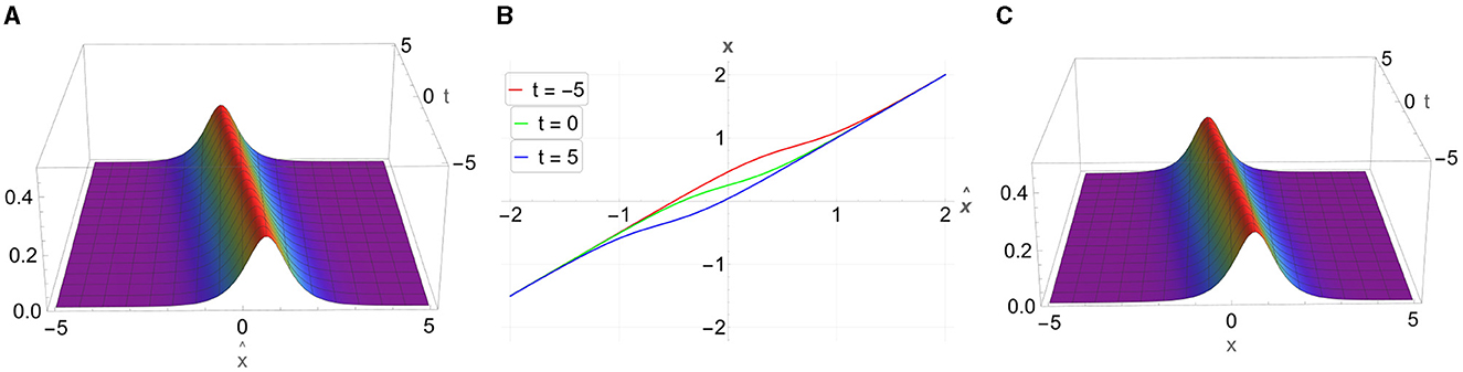
Figure 2. Smooth soliton. (A) $\left|\widehat{u}(\widehat{x},t)\right|$. (B) $x(\widehat{x},t)$ for three values of t. (C) |u(x, t)|.

As expected, in this case, the solution u is smooth both in $\widehat{x}$ and x variables because $\frac{\partial x}{\partial \widehat{x}}$ is nowhere zero.

6.2 Soliton-like solutions associated with a single, double zero of a(k)

Case 3: k₁ = i, α₁ = −2i, β₁ = 4. In this case (see Section 5.2), $E(\widehat{x},t)=\frac{1}{4}{\text{e}}^{-2\widehat{x}-t/2}$ and $F(\widehat{x},t)=(-1-\widehat{x}+\frac{t}{4}){\text{e}}^{-2\widehat{x}-t/2}$. From Equation 87, we get

$\begin{array}{c}\widehat{u}(\widehat{x},t)=\\ \frac{2\text{i}{\text{e}}^{2\widehat{x}+t/2}(4-t+4\widehat{x}+4{\text{e}}^{4\widehat{x}+t}(t-4(2+\widehat{x})))}{1+16{\text{e}}^{8\widehat{x}+2t}+4{\text{e}}^{4\widehat{x}+t}(38+t^2+48\widehat{x}+16{\widehat{x}}^2-4t(3+2\widehat{x}))}.\end{array}$

In this case, the solution is purely imaginary, and we can plot its imaginary part, see Figures 3A, C. The spatial coordinate relation is (Figure 3B)

$\begin{array}{c}x(\widehat{x},t)=\\ \widehat{x}+1+\frac{1-16{\text{e}}^{8\widehat{x}+2t}-8e^{4\widehat{x}+t}(-6+t-4\widehat{x})}{1+16{\text{e}}^{8\widehat{x}+2t}+4{\text{e}}^{4\widehat{x}+t}(38+t^2+48\widehat{x}+16{\widehat{x}}^2-4t(3+2\widehat{x}))}.\end{array}$

Figure 3

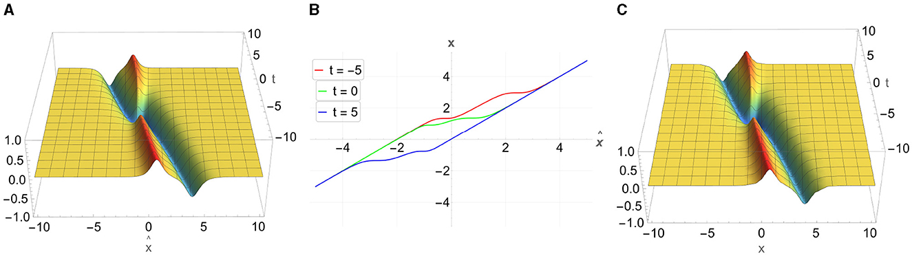
Figure 3. Soliton-type solution associated with a double zero of a(k). (A) $Imu(\widehat{x},t)$. (B) $x(\widehat{x},t)$ for three values of t. (C) Imu(x, t).

7 Conclusion

In the study, we have developed the Riemann–Hilbert approach to a complex-valued integrable modification of the short pulse equation, named as the modified focusing complex short pulse equation (mfcSPE). This equation shares the following property with other Camassa–Holm-type non-linear integrable equations (including the short pulse equation): The Riemann–Hilbert formalism involves a change of variables playing the role of parameters in the associated Riemann–Hilbert problem. Consequently, the representation of the solution of the non-linear PDE in question turns out to be intrinsically parametric, including the construction of the simplest, soliton-like solutions. Particularly, for one-soliton solutions associated with a simple zero of the respective spectral function a(k), we have shown that depending on the location of this zero in the complex plane, the solution either is a smooth function of the original spatial and time variables or has the form of a traveling wave with the cusped hump. Numerical examples illustrate one-soliton solutions associated with both a simple and a double zero of a(k).

Data availability statement

The original contributions presented in the study are included in the article/supplementary material, further inquiries can be directed to the corresponding author.

Author contributions

RB: Data curation, Investigation, Software, Writing – original draft, Writing – review & editing. DS: Conceptualization, Investigation, Methodology, Writing – original draft, Writing – review & editing.

Funding

The author(s) declare that no financial support was received for the research, authorship, and/or publication of this article.

Conflict of interest

The authors declare that the research was conducted in the absence of any commercial or financial relationships that could be construed as a potential conflict of interest.

Publisher's note

All claims expressed in this article are solely those of the authors and do not necessarily represent those of their affiliated organizations, or those of the publisher, the editors and the reviewers. Any product that may be evaluated in this article, or claim that may be made by its manufacturer, is not guaranteed or endorsed by the publisher.

References

1. Ablowitz MJ, Segur H. Solitons and the Inverse Scattering Transform. SIAM Studies in Applied Mathematics, No 4. Philadelphia, PA: SIAM (1981).

Google Scholar

2. Beals R, Coifman RR. Scattering and inverse scattering for first order systems. Comm Pure Appl Math. (1984) 37:39–90. doi: 10.1002/cpa.3160370105

Crossref Full Text | Google Scholar

3. Boutet de Monvel A, Shepelsky D. Riemann-Hilbert approach for the Camassa-Holm equation on the line. C R Math Acad Sci. (2006) 343:627–32. doi: 10.1016/j.crma.2006.10.014

Crossref Full Text | Google Scholar

4. Boutet de Monvel A, Shepelsky D. Riemann-Hilbert problem in the inverse scattering for the Camassa-Holm equation on the line. In: Pinsky M, Birnir B, , editors. Probability, Geometry and Integrable Systems, Vol 55 of Mathematical Sciences Research Institute Publications. Cambridge: Cambridge University Press (2008). p. 53–75.

Google Scholar

5. Boutet de Monvel A, Shepelsky D. A Riemann-Hilbert approach for the Degasperis-Procesi equation. Nonlinearity. (2013) 26:2081–107. doi: 10.1088/0951-7715/26/7/2081

Crossref Full Text | Google Scholar

6. Boutet de Monvel A, Shepelsky D. The Ostrovsky-Vakhnenko equation by a Riemann-Hilbert approach. J Phys A Math Theor. (2015) 48:035204. doi: 10.1088/1751-8113/48/3/035204

Crossref Full Text | Google Scholar

7. Boutet de Monvel A, Shepelsky D, Zielinski L. The short-wave model for the Camassa-Holm equation: a Riemann-Hilbert approach. Inverse Prob. (2011) 27:105006. doi: 10.1088/0266-5611/27/10/105006

Crossref Full Text | Google Scholar

8. Boutet de Monvel A, Shepelsky D, Zielinski L. The short pulse equation by a Riemann-Hilbert approach. Lett Math Phys. 107:1345–73. doi: 10.1007/s11005-017-0945-z

PubMed Abstract | Crossref Full Text | Google Scholar

9. Camassa R, Holm DD. An integrable shallow water equation with peaked solitons. Phys Rev Lett. (1993) 71:1661–4. doi: 10.1103/PhysRevLett.71.1661

PubMed Abstract | Crossref Full Text | Google Scholar

10. Chung Y, Jones CKRT, Schäfer T, Wayne CE. Ultra-short pulses in linear and nonlinear media. Nonlinearity. (2005) 18:1351–74. doi: 10.1088/0951-7715/18/3/021

PubMed Abstract | Crossref Full Text | Google Scholar

11. Clancy K, Gohberg IC. Factorization of Matrix Functions and Singular Integral Operators. Vol 3 of Operator Theory: Advances and Applications. Boston, MA: Birkhäuser Verlag (1981).

Google Scholar

12. Faddeev LD, Takhtajan LA. Hamiltonian Methods in the Theory of Solitons. Springer Series in Soviet Mathematics. Berlin: Springer-Verlag (1987).

Google Scholar

13. Gohberg IC, Krein MG. Systems of integral equations on a half-line with kernels depending on the difference of arguments. Am Math Soc Trans. (1960) 14:217–87. doi: 10.1090/trans2/014/09

Crossref Full Text | Google Scholar

14. Guo BL, Liu N. A Riemann-Hilbert approach for the modified short pulse equation. Appl Anal. (2019) 98:1646–59. doi: 10.1080/00036811.2018.1437418

PubMed Abstract | Crossref Full Text | Google Scholar

15. Matsuno Y. Integrable multi-component generalization of modified short pulse equation. J Math Phys. (2016) 57:11507. doi: 10.1063/1.4967952

Crossref Full Text | Google Scholar

16. Sakovich S. Transformation and integrability of a generalized short pulse equation. Commun Nonlinear Sci Numer Simul. (2016) 39:21–8. doi: 10.1016/j.cnsns.2016.02.031

Crossref Full Text | Google Scholar

17. Sakovich A, Sakovich S. The short pulse equation is integrable. J Phys Soc Japan. (2005) 74:239–41. doi: 10.1143/JPSJ.74.239

Crossref Full Text | Google Scholar

18. Sakovich A, Sakovich S. Solitary wave solutions of the short pulse equation. J Phys A Math Gen. (2006) 39:L361–7. doi: 10.1088/0305-4470/39/22/L03

Crossref Full Text | Google Scholar

19. Schäfer T, Wayne CE. Propagation of ultra-short optical pulse in nonlinear media. Phys D. (2004) 196:90–105. doi: 10.1016/j.physd.2004.04.007

PubMed Abstract | Crossref Full Text | Google Scholar

20. Zhao D, Zhaqilao. On two new types of modified short pulse equation. Nonlinear Dyn. (2020) 100:615–27. doi: 10.1007/s11071-020-05530-9

Crossref Full Text | Google Scholar

21. Zhou X. The Riemann-Hilbert problem and inverse scattering. SIAM J Math Anal. (1989) 20:966–86. doi: 10.1137/0520065

Crossref Full Text | Google Scholar