Disentangling dynamic and stochastic modes in multivariate time series

A signal decomposition is presented that disentangles the deterministic and stochastic components of a multivariate time series. The dynamical component analysis (DyCA) algorithm is based on the assumption that an unknown set of ordinary differential equations (ODEs) describes the dynamics of the deterministic part of the signal. The algorithm is thoroughly derived and accompanied by a link to the GitHub repository containing the algorithm. The method was applied to both simulated and real-world data sets and compared to the results of principal component analysis (PCA), independent component analysis (ICA), and dynamic mode decomposition (DMD). The results demonstrate that DyCA is capable of separating the deterministic and stochastic components of the signal. Furthermore, the algorithm is able to estimate the number of linear and non-linear differential equations and to extract the corresponding amplitudes. The results demonstrate that DyCA is an effective tool for signal decomposition and dimension reduction of multivariate time series. In this regard, DyCA outperforms PCA and ICA and is on par or slightly superior to the DMD algorithm in terms of performance.

1 Introduction

Multivariate signal processing is important in a broad spectrum of applications for understanding complex systems, improving signal quality, making accurate predictions, and extracting meaningful information from multivariate data sources.

One way of analyzing multivariate data, especially multivariate (vector) time series, is to decompose the signal into relevant components (modes and vectors) and their corresponding amplitudes (time series). This leads to a matrix factorization and by looking at the resulting amplitudes to a dimension reduction of the signal. The approach may also be regarded as a form of signal filtration, i.e., a separation of relevant and irrelevant components. Fields of application are manifold and include the analysis of climate data, e.g., [1], financial time series, e.g., [2], medical data, e.g., artifact removal in electroencephalographic data [3], speech recognition, e.g., [4], modern farming, e.g., [5], and many more.

The most widely used techniques for signal decomposition are based on principal component analysis (PCA) [6, 7] and are used in a wide range of applications—sometimes called by different names, such as Karhunen-Loève transform (KLT), proper orthogonal decomposition (POD), eigenvalue decomposition (EVD), empirical orthogonal functions (EOF), empirical eigenfunction decomposition, and empirical modal analysis. PCA decomposes the signal into a set of orthogonal components (modes) and their corresponding amplitudes (time series) such that the variance of the components is maximized. The components are ordered by their variance, and the first components capture the most variance of the signal. It is a well-established technique for dimension reduction but has some limitations due to its linear character. A variety of extensions have been developed to overcome these limitations. We would like to mention two of them: kernel PCA, calculating principal components in high-dimensional feature spaces, related to the input space by some non-linear map [8], and non-linear PCA, based on auto-associative neural networks (autoencoder) [9].

Another way of extending PCA is to consider time leads and lags in the decomposition of the signal leading to a generalized dynamic PCA [2]. Shifting the focus of the decomposition on the dynamics of a multivariate signal is realized by the field of dynamic mode decompositions (DMD) [10] and its extensions based on Koopman operator theory [11, 12]. Principal interaction and oscillation patterns (PIPs and POS) [13] are precursors to the concept of DMD.

However, another very common approach to decompose a multivariate signal is given by independent component analysis (ICA) [14] based on the statistical assumption that the relevant components of the signals are statistically independent non-Gaussian signals. Different techniques have been developed to estimate the independent components with FastICA [15, 16] as the most widely used algorithm.

Our approach, called dynamical component analysis (DyCA) and first presented in Seifert et al. [17] and Korn et al. [18], is based on a separation of amplitudes that are not statistically independent as in ICA, but dynamically coupled by a set of ordinary differential equations (ODEs). DyCA is related to the concepts of dynamic PCA and DMD, as it also focuses on signal dynamics and analyzes its time-lagged representation [19]. With respect to its possible applications, DyCA lies in between ICA and DMD: the signal is separated as in ICA, but the underlying criterion is based on dynamics as in DMD and Koopman operator theory.

The report is organized as follows: In the subsequent section, we present the case of application and the underlying assumptions. The derivation of the DyCA algorithm, a brief summary of the utilized methods for comparison with DyCA and the setup of the investigated examples are introduced in Section 3. In Section 4, we present the results of the application of DyCA to the examples and conclude with a discussion in Section 5.

2 Materials and equipment

Starting point is a multivariate signal Q ∈ ℝ^N×T with N vector-valued components q_i(t) and t = t₁, …, t_T, (t_i−1 − t_i = Δt) representing the time discrete evolution with T > N:

$\begin{array}{ll}Q=\left[\begin{array}{c}{q}_1(t)\\ ⋮\\ q_N(t)\end{array}\right]=\left[\begin{array}{ccc}{q}_1(t_1)& \cdots & q_1(t_T)\\ ⋮& \ddots & ⋮\\ q_N(t_1)& \cdots & q_N(t_T)\end{array}\right]& (1)\end{array}$

We assume that

• the signal splits into a deterministic part Q_D, independent component noise Q_CN, and additive noise Q_AN,

$\begin{array}{ll}Q=Q_D+Q_{CN}+Q_{AN},& (2)\end{array}$

• both deterministic part and component noise can be decomposed into vector-valued independent components W and Ψ and corresponding amplitudes X and Ξ, such that

$\begin{array}{c}{Q}_D=WX\text{ and }{Q}_{CN}=\text{Ψ}\Xi ,\text{ with }W\in {ℝ}^{N\times n},\\ \text{Ψ}\in {ℝ}^{N\times p},X\in {ℝ}^{n\times T},\Xi \in {ℝ}^{p\times T},& (3)\end{array}$

• the amplitudes Ξ of the component noise are random,

• the dynamics of the amplitudes X of the deterministic part obey a set of ordinary differential equations (ODEs) with m linear and n − m non-linear equations. The coefficient matrix A (with elements a_ij) corresponding to the linear part is denoted by $A=\left[A_1,A_2\right]\in {ℝ}^{m\times n}$ with $A_1\in {ℝ}^{m\times m}$ and $A_2\in {ℝ}^{m\times (n-m)}$ such that Ẋ_L = AX. By the notation Ẋ, we refer to the derivatives of the vector components x_i with respect to time evaluated at all time steps t:

$\begin{array}{c}X=\left[\begin{array}{c}{x}_1(t)\\ ⋮\\ x_m(t)\\ x_{m+1}(t)\\ ⋮\\ x_n(t)\end{array}\right]=\left[\begin{array}{c}{X}_L\\ X_{NL}\end{array}\right],Ẋ=\left[\begin{array}{c}{Ẋ}_L\\ {Ẋ}_{NL}\end{array}\right]=\left[\begin{array}{c}AX\\ f(X)\end{array}\right]\\ =\left[\begin{array}{c}{A}_1{X}_L+A_2{X}_{NL}\\ f(X)\end{array}\right].& (4)\end{array}$

The function $f\in {\mathcal{C}}^{\infty }({ℝ}^{n\times T},{ℝ}^{(n-m)\times T})$ is an unknown, non-linear, smooth function and remains unknown in the discussed algorithm.

Note that these assumptions allow for a possible transformation T ∈ GL(n) of X preserving the structure of the set of ODEs: Consider the partition

$\begin{array}{cc}T=\left[\begin{array}{cc}{T}_{11}& T_{12}\\ T_{21}& T_{22}\end{array}\right]& (5)\end{array}$

where $T_{11}\in {ℝ}^{m\times m}$, $T_{21}\in {ℝ}^{(n-m)\times m}$, $T_{12}\in {ℝ}^{m\times (n-m)}$, and $T_{22}\in {ℝ}^{(n-m)\times (n-m)}$ and write $\tilde{W}=W{T}^{-1}$, $\tilde{X}=TX$ and $\dot{\tilde{X}}=TẊ$. The ODE condition yields

$\begin{array}{c}\dot{\tilde{X}}=TẊ\\ =\left[\begin{array}{cc}{T}_{11}& T_{12}\\ T_{21}& T_{22}\end{array}\right]\left[\begin{array}{c}A(T^{-1}\tilde{X})\\ f(T^{-1}\tilde{X})\end{array}\right]=\left[\begin{array}{c}{T}_{11}A{T}^{-1}\tilde{X}+T_{12}f(T^{-1}\tilde{X})\\ T_{21}A{T}^{-1}\tilde{X}+T_{22}f(T^{-1}\tilde{X})\end{array}\right].& (6)\end{array}$

In order to preserve the structure of the ODE, the above computation shows that $T_{12}f(T^{-1}\tilde{X})=0$ needs to be fulfilled for all $\tilde{X}$. A sufficient condition is T₁₂ = 0. Assuming T₁₂ = 0, one obtains that T has the following block structure

$\begin{array}{cc}T=\left[\begin{array}{cc}{T}_{11}& 0\\ T_{21}& T_{22}\end{array}\right]\in \text{GL}(n)\text{ and }\dot{\tilde{X}}=\left[\begin{array}{c}\tilde{A}\tilde{X}\\ \tilde{f}(\tilde{X})\end{array}\right]& (7)\end{array}$

holds, where $\tilde{A}=T_{11}A{T}^{-1}$ and $\tilde{f}(\tilde{X})=T_{21}A{T}^{-1}\tilde{X}+T_{22}f(T^{-1}\tilde{X})$.

3 Methods

3.1 DyCA algorithm

We present a comprehensive derivation that summarizes Uhl et al. [20] and Romberger et al. [21] with some important improvements concerning the algorithm to extract all relevant amplitudes. The Python implementation of the algorithm has been released recently and is publicly available¹.

Goal of dynamical component analysis (DyCA) is to disentangle the deterministic amplitudes X of the signal Q based on the structure of the assumed dynamics (Equation 4). It is based on minimizing the least square error of Ẋ_L = AX. To obtain a unique solution with respect to possible scaling of the amplitudes, the constraint $diag({Ẋ}_L{Ẋ}_L^T)=I_m$ is considered:

$\begin{array}{cc}{\displaystyle \underset{X,A}{min}}\parallel {Ẋ}_L-AX{\parallel }^2\text{ s.t. }diag({Ẋ}_L{Ẋ}_L^T)=I_m.& (8)\end{array}$

The freedom described in Equation 7 will be discussed later.

As there exists a generalized left inverse U ∈ ℝ^n×N such that UW = I_n and UΨ = 0, the amplitudes X are approximated by X ≃ UQ in the case of low additive noise Q_AN. Therefore, the partition of X into $X=\left[\begin{array}{c}{X}_L\\ X_{NL}\end{array}\right]$ is given by $U=\left[\begin{array}{c}{U}_L\\ U_{NL}\end{array}\right]\in {ℝ}^{n\times N}$ with $U_L\in {ℝ}^{m\times N}$ and $U_L\in {ℝ}^{(n-m)\times N}$. This leads to the optimization problem with respect to the unknown matrices U and A:

$\begin{array}{cc}{\displaystyle \underset{U,A}{min}}\parallel U_L\dot{Q}-AUQ{\parallel }^2\text{ s.t. }diag((U_L\dot{Q}){(U_L\dot{Q})}^T)=I_m.& (9)\end{array}$

Introducing correlation matrices C₀, C₁ and $C_2\in {ℝ}^{N\times N}$

$\begin{array}{cc}{C}_0=Q{Q}^T,C_1=\dot{Q}{Q}^T,C_1=\dot{Q}{\dot{Q}}^T,& (10)\end{array}$

and a diagonal Lagrange parameter matrix Σ ∈ ℝ^m×m with diagonal elements σ₁, …, σ_m ∈ ℝ, we obtain from Equation 9 a cost function g,

$\begin{array}{c}g(U,A,\Sigma )=tr(U_L{C}_2{U}_L^T)-2tr(U_L{C}_1{U}^T{A}^T)\\ +tr(AU{C}_0{U}^T{A}^T)+tr(\Sigma (U_L{C}_2{U}_L^T-I_m)).& (11)\end{array}$

The critical points of g are obtained by setting the partial directional derivatives of g with respect to the three matrix-valued arguments U, A, Σ to zero leading to the following expressions:

$\begin{array}{cc}{C}_2{U}_L^T(I_m+\Sigma )-C_1{U}^T{A}^T-(C_1^T{U}_L-C_0{U}^T{A}^T)A=0,& (12)\end{array}$

$\begin{array}{cc}U(C_0{U}^T{A}^T-C_1^T{U}_L)=0,& (13)\end{array}$

$\begin{array}{cc}diag(U_L{C}_2{U}_L^T)-I_m=0.& (14)\end{array}$

A sufficient condition is given by

$\begin{array}{r}{C}_2{U}_L^T(I_m+\Sigma )=C_1{U}^T{A}^T,C_0{U}^T{A}^T=C_1^T{U}_L,\\ diag{U}_L{C}_2{U}_L^T=I_m,& (15)\end{array}$

which bears resemblance to the characteristic DyCA equations presented in Uhl et al. [20] if we introduce the diagonal matrix Λ: = I_m + Σ (with diagonal elements λ_i) and a matrix V: = AU, reflecting the degree of freedom described in Equation 7:

$\begin{array}{cc}{C}_2{U}_L^T\Lambda =C_1{V}^T,C_0{V}^T=C_1^T{U}_L,U_L{C}_2{U}_L^T=I_m.& (16)\end{array}$

As we assume a full rank signal Q², the correlation matrix C₀ is regular, and therefore, the second equation in Equation 16 can be solved for V^T,

$\begin{array}{cc}{V}^T=C_0^{-1}{C}_1^T{U}_L.& (17)\end{array}$

Inserting this into the first equation by Equation 16, the generalized eigenvalue problem

$\begin{array}{cc}{C}_1{C}_0^{-1}{C}_1^T{U}_L=C_2{U}_L^T\Lambda & (18)\end{array}$

is obtained for solving Equation 16.

Evaluating the critical point (Equation 16) in the cost function (Equation 11) yields the minimal value g_min = −tr(Σ) = m − tr(Λ), i.e., the generalized eigenvalues λ_i with 0 ≤ λ_i ≤ 1 measure the goodness of fit concerning the linear part of the dynamics (Equation 8): A value close to 1 indicates a good match for the amplitude x_i(t) with

$\begin{array}{cc}{ẋ}_i(t)\simeq {\displaystyle \sum _{j=1}^n}{a}_{ij}{x}_j(t).& (19)\end{array}$

Thresholding with an appropriate parameter α the spectrum of the generalized eigenvalues λ_i of Equation 18 yields an estimate $\widehat{m}$ of m,

$\begin{array}{cc}\widehat{m}=\left|\left\{{\lambda }_i|{\lambda }_i>\alpha \right\}\right|,& (20)\end{array}$

and the corresponding $U_L\in {ℝ}^{\widehat{m}\times N}$ an estimate of the amplitudes ${\widehat{X}}_L$:

$\begin{array}{cc}{\widehat{X}}_L=U_{L}Q.& (21)\end{array}$

An estimate of the amplitudes ${\widehat{X}}_{NL}$ has to be extracted from the amplitudes VQ. By construction of V: = AU the amplitudes X_L are included in the linear combination of AX = A₁X_L + A₂X_NL, therefore disentangling the amplitudes can only be solved except possible transformations (Equation 7). For an equally weighted comparison of the amplitudes, we use thresholding the economy-size singular value decomposition (SVD) of the normalized matrix $\left[\begin{array}{c}{N}_L{U}_{L}Q\\ N_{V}VQ\end{array}\right]:=\left[\begin{array}{c}{Ũ}_{L}Q\\ ṼQ\end{array}\right]\in {ℝ}^{2\widehat{m}\times T}$ with diagonal matrices $N_L,N_V\in {ℝ}^{\widehat{m}\times \widehat{m}}$ and $diag({Ũ}_L{C}_0{Ũ}_L^T)=diag(ṼC_0{Ṽ}^T)=I_{\widehat{m}}$. Let the economy-size SVD be given by BSY^T,

$\begin{array}{cc}\left[\begin{array}{c}{Û}_{L}Q\\ \widehat{V}Q\end{array}\right]=BS{Y}^T,& (22)\end{array}$

with matrices $B\in {ℝ}^{2\widehat{m}\times 2\widehat{m}}$, $Y\in {ℝ}^{2\widehat{m}\times T}$, rectangular diagonal matrix $S\in {ℝ}^{2\widehat{m}\times 2\widehat{m}}$, and diagonal elements $s_1,s_2,\dots s_{2\widehat{m}}$. The dimensionality of the embedded signal $\widehat{n}$ can now be estimated by an appropriate threshold β with

$\begin{array}{cc}\widehat{n}=\left|\left\{s_i|s_i/tr(S)>\beta \right\}\right|.& (23)\end{array}$

and rearranged amplitudes are then approximated by

$\begin{array}{cc}\widehat{X}=BŜY^T& (24)\end{array}$

with a truncated rectangular diagonal matrix Ŝ and diagonal elements $s_1,s_2,\dots s_{\widehat{n}}$.

Note that this approach of introducing a corresponding pair of matrices U_L and V can only approximate the dimension of the embedded signal n if n ≤ 2m; i.e., the number m of linear differential equations must be greater than or equal to the number n − m of non-linear differential equations: m ≥ n − m. Moreover, note that, second, the approximation of the relevant amplitudes and the corresponding dimension is an improvement over the previous approach in Uhl et al. [20], as it is now based on the possible amplitudes ${\left[\begin{array}{c}{Ũ}_{L}Q,ṼQ\end{array}\right]}^T$ instead of the projection vectors ${\left[\begin{array}{c}{U}_L,V\end{array}\right]}^T$ alone.

3.2 Dimension reduction methods PCA, ICA, and DMD

The examples of application are compared to the results of the PCA, ICA, and DMD algorithms. The PCA algorithm is based on solving the eigenvalue problem of the correlation matrix C₀. The eigenvalues of the correlation matrix will be denoted in the following with p_i. The utilized ICA algorithm is the kurtosis-based FastICA algorithm [15].

The DMD algorithm [12] is based on the eigenvalues of the best-fit linear matrix operator B that approximates the time evolution of the signal:

$\begin{array}{cc}{q}_i(t+1)=B{q}_i(t).& (25)\end{array}$

The matrix B is calculated by the pseudoinverse of signal Q and the time-lagged signal Q′. The eigenvalues of B will be denoted in the following with μ_i. The amplitudes corresponding to the eigenvectors Φ_i are calculated by the inverse of the eigenvectors, Φ⁻¹Q, and rearranged to obtain real-valued amplitudes from the complex conjugate pairs. Mode selection is performed by considering modes with the largest absolute value of its eigenvalues.

3.3 Examples of application

Different examples of simulated and real-world data are presented to demonstrate the performance and the limitations of the DyCA algorithm. Details of the signals will be presented below. The derivatives of the signals Q—both, simulated signal and EEG signal—are approximated by the central finite difference scheme with a given time step of Δt: $\dot{Q}(t)=(Q(t+\Delta t)-Q(t-\Delta t))/(2\Delta t)$. Note that this is a major source of inaccuracy. If better derivatives (measurement, filter) are available, the performance of the DyCA algorithm will be improved.

3.3.1 Simulated examples

The simulated examples consist of full rank signals Q ∈ ℝ^N×T with N = 20 and T = 100, fulfilling the assumptions (Equations 2, 3). The additive noise Q_AN is assumed to be standard normally distributed with a signal-to-noise ratio (SNR) of 50 dB. The deterministic part Q_D is generated by numerical integration (standard explicit Runge–Kutta (4, 5) procedure [22]) of the given set of ODEs with predefined initial conditions and a sampling rate of 100 Hz. The signals are resampled with a time step Δt = 0.18 s and form the matrix $X={\left[x_1(t),\dots ,x_n(t)\right]}^T$. The component noise Q_CN consists of two random amplitudes ξ₁(t), ξ₂(t), i.e., p = 2, that form the matrix $\Xi ={\left[{\xi }_1(t),{\xi }_2(t)\right]}^T$. Both the deterministic amplitudes and the stochastic amplitudes are shown for each example. The components W and Ψ are generated by random numbers drawn from the uniform distribution in the interval (0,1). The SNR of the component noise Q_CN is set to 0 dB.

Three different simulated examples are presented:

1. Van der Pol oscillator: The Van der Pol oscillator [23] is a two-dimensional (n = 2) oscillator with one linear (m = 1) and one non-linear differential equation. The ODEs are given by

$\begin{array}{l}{ẋ}_1(t)=x_2(t)\\ {ẋ}_2(t)=-x_1(t)+ϵ(1-x_1{(t)}^2)x_2(t).& (26)\end{array}$

For the simulation, the parameter ϵ is set ϵ = 5.

2. Rössler attractor: The Rössler attractor [24] is a chaotic attractor with two linear (m = 2) and one non-linear governing differential equation:

$\begin{array}{l}{ẋ}_1(t)=-x_2(t)-x_3(t)\\ {ẋ}_2(t)=x_1(t)+a{x}_2(t)\\ {ẋ}_3(t)=b+x_3(t)(x_1(t)-c)& (27)\end{array}$

and selected parameters a = 0.15, b = 0.2 and c = 10.

3. Lorenz attractor: The Lorenz attractor [25] does not fulfill the DyCA requirements. The underlying set of differential equations consists of one linear (m = 1) and two non-linear differential equations:

$\begin{array}{l}{ẋ}_1(t)=\alpha (x_2(t)-x_1(t))\\ {ẋ}_2(t)=x_1(t)(\beta -x_3(t))-x_2(t)\\ {ẋ}_3(t)=x_1(t)x_2(t)-\gamma x_3(t)& (28)\end{array}$

with the parameters α = 10, β = 28 and γ = 8/3.

3.3.2 Electroencephalographic signal

As a real-world example, we consider a multivariate EEG signal Q ∈ ℝ^N×T with N = 25 and T = 1, 000 representing the time discrete evolution of an EEG signal during an epileptic so-called petit-mal seizure. The 25 channels are recorded and labeled according to the modified 10/20 system. The signal is recorded with a sampling rate of 256 Hz and preprocessed by a zero-phase bandpass filter with a passband of 0.5–30 Hz. This dataset is kindly provided by the Epilepsy Center at the Department of Neurology Erlangen. The motivation to analyze this type of EEG data with DyCA is based on physiological findings that Shilnikov chaos can be observed in the brain during petit-mal seizures [26]. This type of chaos is governed by a three-dimensional set of differential equations with two linear and one non-linear ODE, thus fulfilling the assumptions for the application of DyCA. This occurrence of Shilnikov chaos in EEG data of petit-mal epileptic seizures has been confirmed by our data-driven approach presented in Seifert et al. [17].

4 Results

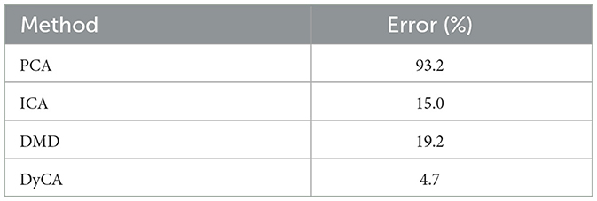
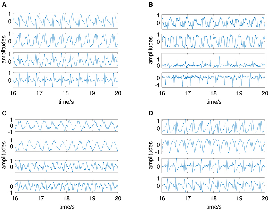
For all investigated datasets, the characteristic values (eigenvalues of PCA and DMD, generalized eigenvalues of DyCA, and singular values of possible DyCA amplitudes) are shown in one figure. Due to the invariance of the amplitudes with respect to a linear transformation³ D the amplitudes are transformed to minimize the Frobenius norm of the difference between the estimated amplitudes $\widehat{X}$ and the simulated amplitudes X, $D={argmin}_D\left|\right|X-D\widehat{X}\left|\right|$. These transformed estimated amplitudes $D\widehat{X}$ are shown for each simulated dataset and for each algorithm in a second figure (original deterministic amplitudes in blue, transformed estimated amplitudes in red). In addition to this visual impression, a quantitative measure of the performance of the different algorithms is provided in a table. For each simulated dataset, the table summarizes the relative errors of the Frobenius norm of the difference between the estimated amplitudes $D\widehat{X}$ and the simulated amplitudes X.

4.1 Simulated examples

1. Van der Pol oscillator

The amplitudes both deterministic, x₁(t) and x₂(t), and stochastic, ξ₁(t) and ξ₂(t), are shown in Figure 1A, and the resulting multivariate signal Q is shown in Figure 1B. The deterministic amplitudes show a limit cycle behavior, and the stochastic amplitudes are uncorrelated. Figure 2B shows on the left side four non-vanishing PCA eigenvalues p_i consistent with the simulation of two (n = 2) deterministic and two (p = 2) stochastic amplitudes. The two dominant corresponding amplitudes are shown in Figure 3A. They represent a mixture of the deterministic and stochastic amplitudes as deterministic and stochastic components are equally distributed in the simulation (SNR is set to 0 dB). The amplitudes obtained by FastICA are shown in Figure 3B. They show a high degree of correlation with the simulated deterministic amplitudes. The eigenvalues of the DMD algorithm μ_i are shown in Figure 2A. Mode selection based on the absolute value of the complex eigenvalues can be clearly performed, and two dominant modes with large absolute values are observed—consistent with the simulation of two deterministic amplitudes. This is confirmed by the amplitudes shown in Figure 3C. The DyCA algorithm yields the generalized eigenvalues λ_i, which are displayed in the center of Figure 2B. One generalized eigenvalue is close to 1 corresponding to the simulation based on one linear differential equation. The singular values s_i on the right-hand side of Figure 2B show that the DyCA algorithm is able to extract the two deterministic amplitudes. The amplitudes are shown in Figure 3D and illustrate the separation of the deterministic and stochastic amplitudes. Table 1 summarizes the relative errors of the Frobenius norm of the difference between the estimated amplitudes and the simulated amplitudes and show that DyCA yields for that example the best results.

2. Roessler attractor

Deterministic and stochastic amplitudes are shown in Figure 4A and the resulting multivariate signal in Figure 4B. Similar to the Van der Pol oscillator, the results are consistent with the simulation: we observe five PCA eigenvalues p_i ≠ 0, due to three (n = 3) deterministic and two (p = 2) stochastic amplitudes (left side of Figure 5B). Mode selection of the DMD algorithm based on the DMD eigenvalues (Figure 5A) yields three modes, and DyCA indicates two linear differential equations ($\widehat{m}=2$) by two generalized eigenvalues close to 1 (center of Figure 5B). The spectrum of the singular values yields three deterministic modes ($\widehat{n}=3$) (right side of Figure 5B). The three obtained transformed amplitudes by PCA, FastICA, DMD, and DyCA are shown in Figure 6. DMD and DyCA clearly deliver the best results. The quantitative summary of these findings is given in Table 2. DMD and DyCA lead by far better results than PCA and FastICA, again DyCA with the best results.

3. Lorenz attractor

Again the deterministic and stochastic amplitudes are shown (Figure 7A) and all channels of the multivariate signal in Figure 7B. Five non-vanishing PCA eigenvalues are observed (Figure 8B, left side), as the simulation consists of three (n = 3) deterministic and two (p = 2) stochastic amplitudes. In the case of DMD, mode selection is challenging: DMD yields one dominant mode with respect to the absolute value of the complex DMD eigenvalues, in addition to two less obvious yet discernible modes (Figure 8A). DyCA indicates one linear differential equation ($\widehat{m}=1$) by one generalized eigenvalue close to 1 (center of Figure 8B). This corresponds to the fact that the Lorenz attractor consists of one linear and two non-linear ODE. This is correctly detected by DyCA but does not lead to a correct signal decomposition, as the requirements are not fulfilled. Nevertheless, to make a comparison of the methods, we assume that DyCA would yield two linear equations, which also might be interpreted from the spectrum of the generalized eigenvalues and we chose $\widehat{n}=3$ from the spectrum of the singular values (Figure 8B, right side). The transformed amplitudes by PCA, FastICA, DMD and DyCA are shown in Figure 9. One observes that only DMD yields amplitudes related to the simulated amplitudes. This is quantitatively summarized in Table 3. Note that looking at the first two amplitudes—which then would fulfill the DyCA requirements—we get good results with DyCA and even better than DMD.

Figure 1

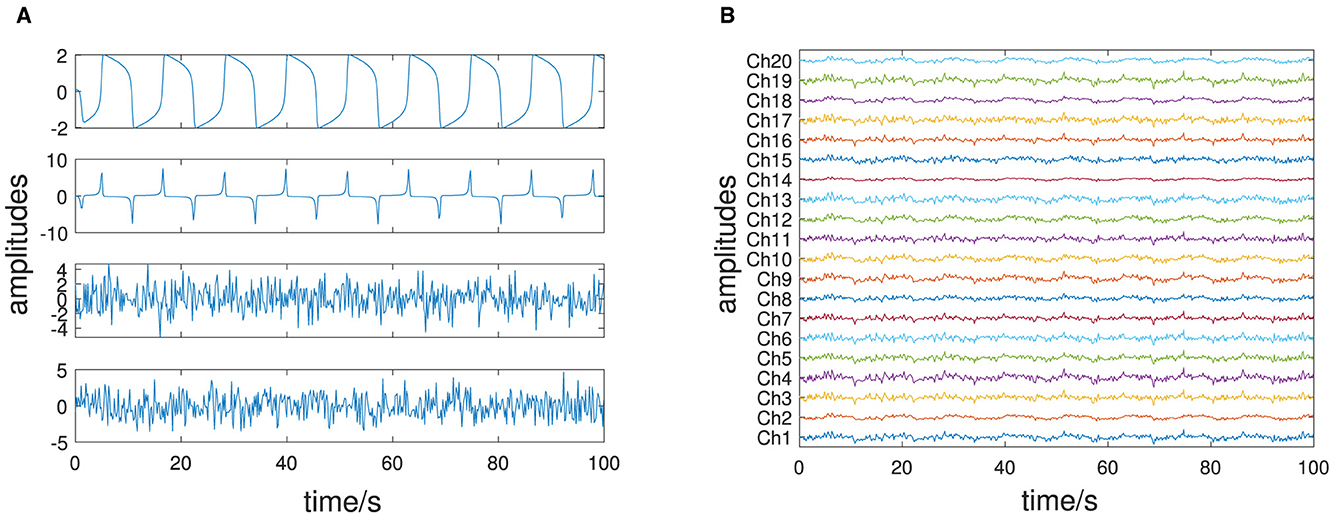
Figure 1. Van der Pol oscillator: (A) deterministic amplitudes x₁(t), x₂(t) (forming X) and stochastic amplitudes ξ₁(t), ξ₂(t) (forming Ū); (B) all channels of the multivariate signal Q = XW + ΞΨ.

Figure 2

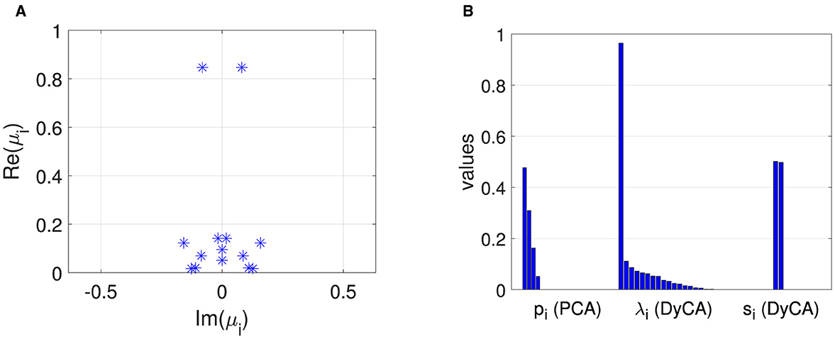
Figure 2. Van der Pol oscillator: (A) complex DMD eigenvalues μ_i, (B) characteristic values: PCA eigenvalues p_i, DyCA generalized eigenvalues λ_i, and SVD values s_i of temporary DyCA amplitudes.

Figure 3

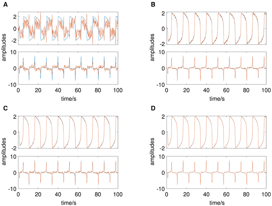
Figure 3. Van der Pol oscillator: original deterministic amplitudes in blue, transformed estimated amplitudes in red, estimated by: (A) PCA, (B) ICA, (C) DMD, and (D) DyCA.

Table 1

Table 1. Van der Pol oscillator: relative error of the estimated amplitudes.

Figure 4

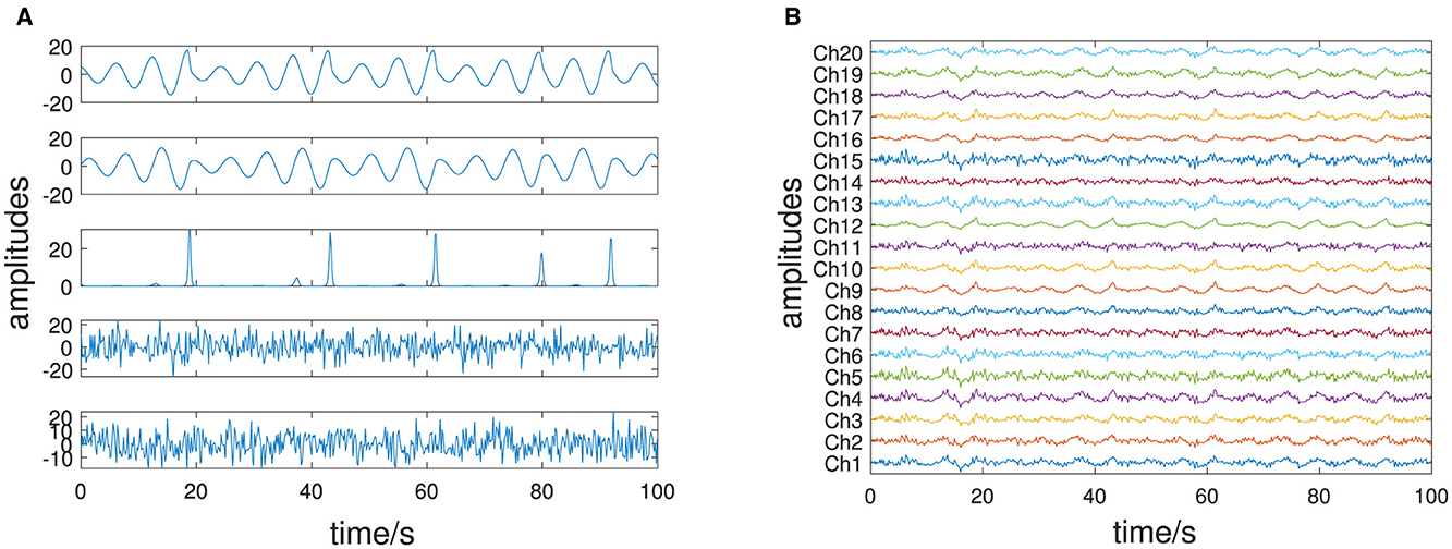
Figure 4. Roessler attractor: (A) deterministic amplitudes x₁(t), x₂(t), x₃(t) (forming X) and stochastic amplitudes ξ₁(t), ξ₂(t) (forming Ξ); (B) all channels of the multivariate signal Q = XW + ΞΨ.

Figure 5

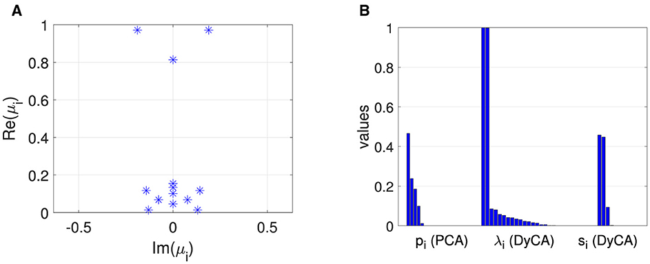
Figure 5. Roessler attractor: (A) complex DMD eigenvalues μ_i, (B) characteristic values: PCA eigenvalues p_i, DyCA generalized eigenvalues λ_i and SVD values s_i of temporary DyCA amplitudes.

Figure 6

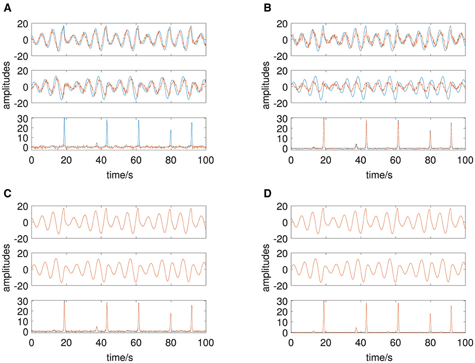
Figure 6. Roessler attractor: original deterministic amplitudes in blue, transformed estimated amplitudes in red, estimated by: (A) PCA, (B) ICA, (C) DMD, and (D) DyCA.

Table 2

Table 2. Roessler attractor: relative error of the estimated amplitudes.

Figure 7

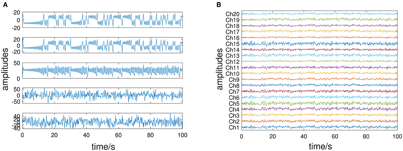
Figure 7. Lorenz attractor: (A) deterministic amplitudes x₁(t), x₂(t), x₃(t) (forming X) and stochastic amplitudes ξ₁(t), ξ₂(t) (forming Ū); (B) all channels of the multivariate signal Q = XW + ΞΨ.

Figure 8

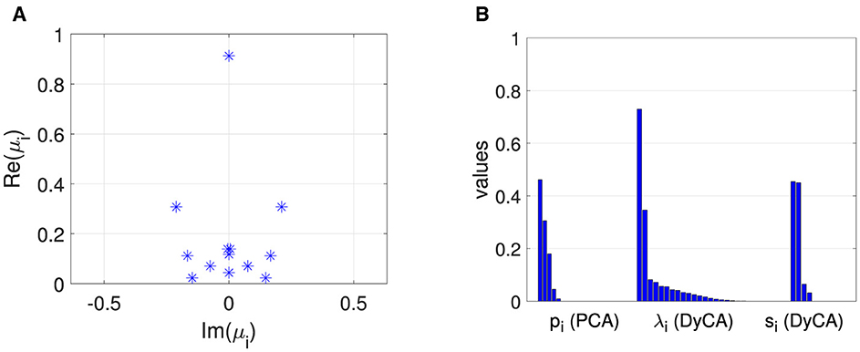
Figure 8. Lorenz attractor: (A) complex DMD eigenvalues μ_i, (B) characteristic values: PCA eigenvalues p_i, DyCA generalized eigenvalues λ_i and SVD values s_i of temporary DyCA amplitudes.

Figure 9

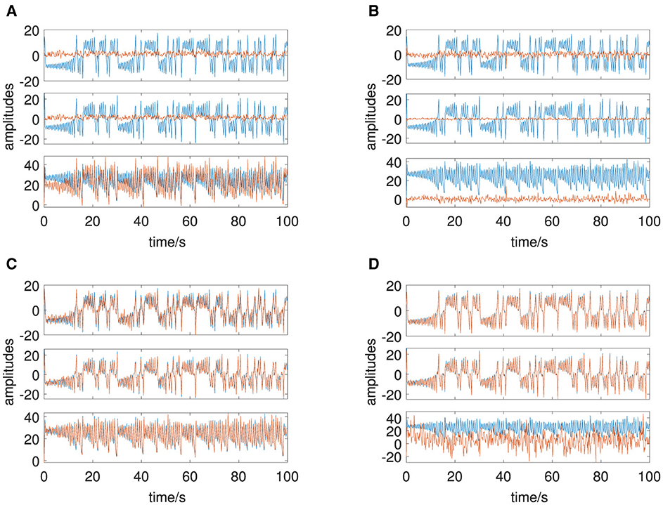
Figure 9. Lorenz attractor: original deterministic amplitudes in blue, transformed estimated amplitudes in red, estimated by: (A) PCA, (B) ICA, (C) DMD, and (D) DyCA.

Table 3

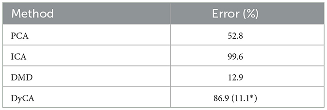
Table 3. Lorenz attractor: relative error of the estimated amplitudes (^* in the case of two amplitudes).

4.2 EEG data

The multivariate EEG signal of an epileptic seizure dicussed in Section 3.3.2 is shown in Figure 10. The left side of Figure 11B shows the PCA eigenvalue spectrum. There are two dominant components which is due to the coherent structure of the petit-mal epileptic seizure. Mode selection is for both DMD and DyCA a difficult task. The DMD complex eigenvalues (Figure 11A) do not separate with respect to the absolute value. The separation of the generalized DyCA eigenvalue spectrum (center of Figure 11B) is not that obvious as in the case of the simulated examples. However one could argue that there are two generalized eigenvalues close to 1, leading to an estimate of $\widehat{m}=2$ underlying linear differential equations. The spectrum of the singular values (right side of Figure 11B) indicates $\widehat{n}=4$ components. The amplitudes obtained by PCA, FastICA, DMD, and DyCA are shown in Figure 12. Similarities between PCA and DyCA amplitudes are clearly visible, whereas DMD and ICA yield different results. The obtained DyCA amplitudes confirm the findings of Seifert et al. [27] where low-dimensional Shilnikov chaos was detected in the EEG data sets.

Figure 10

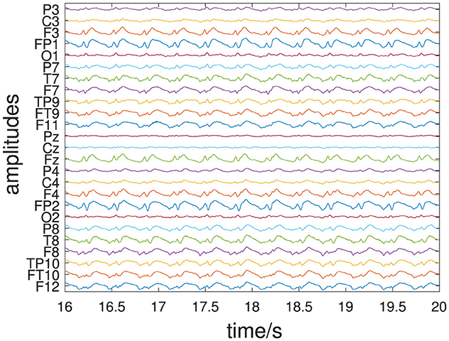
Figure 10. EEG signal: all channels of the multivariate signal, each channel labeled in the modified 10/20 system.

Figure 11

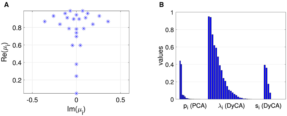
Figure 11. EEG signal: (A) complex DMD eigenvalues μ_i, (B) characteristic values: PCA eigenvalues p_i, DyCA generalized eigenvalues λ_i and SVD values s_i of temporary DyCA amplitudes.

Figure 12

Figure 12. EEG signal: estimated amplitudes, estimated by: (A) PCA, (B) ICA, (C) DMD, and (D) DyCA.

5 Discussion

We have demonstrated that DyCA is capable of extracting the deterministic amplitudes of a signal and separating them from stochastic amplitudes under certain conditions. These conditions are as follows: (a) the signal is divided into a deterministic part, independent component noise, and low additive noise; (b) both the deterministic part and component noise can be decomposed into independent components; and (c) the number of linear differential equations is equal to or greater than the number of non-linear differential equations. The spectrum of the generalized DyCA eigenvalues allows for the verification of the fulfillment of the aforementioned conditions. The number of generalized eigenvalues close to 1 provides an estimate of the number of linear differential equations. The spectrum of the singular values of the amplitudes corresponding to the generalized eigenvectors and the amplitudes of the associated vectors provides an estimate of the dimension of the deterministic subspace. In the aforementioned circumstances, DyCA outperforms PCA and ICA and is comparable or slightly more effective than the DMD algorithm. A comprehensive study comparing DyCA with DMD with respect to noise robustness and sampling frequency can be found in Stiehl et al. [28]. In the case of more non-linear than linear ODEs governing the system under investigation, DyCA can still be used to estimate the number of linear ODEs and two times as many amplitudes as demonstrated by the example of the simulated Lorenz attractor. The analysis of a multivariate EEG signal demonstrates the potential of DyCA to extract the deterministic amplitudes of complex real-world signals.

Ultimately, the objective was to provide a detailed account of the DyCA algorithm and its implementation, which can be utilized by the provided Python package on GitHub as a valuable tool for the analysis of multivariate signals. This may serve as a basis for further explorations in various directions.

Data availability statement

The raw data supporting the conclusions of this article will be made available by the authors, without undue reservation.

Ethics statement

Ethical approval was not required for the study involving humans in accordance with the local legislation and institutional requirements. Written informed consent to participate in this study was not required from the participants or the participants' legal guardians/next of kin in accordance with the national legislation and the institutional requirements.

Author contributions

CU: Investigation, Methodology, Writing – original draft. AS: Investigation, Methodology, Writing – original draft. NW: Investigation, Methodology, Writing – original draft. MS: Investigation, Methodology, Writing – original draft. KH: Investigation, Methodology, Writing – original draft.

Funding

The author(s) declare financial support was received for the research, authorship, and/or publication of this article. This study has been supported by the German Federal Ministry of Education and Research (BMBF-Projekt, funding numbers: 05M20WWA and 05M20WBA Verbundprojekt 05M2020—DyCA).

Conflict of interest

The authors declare that the research was conducted in the absence of any commercial or financial relationships that could be construed as a potential conflict of interest.

The author(s) declared that they were an editorial board member of Frontiers, at the time of submission. This had no impact on the peer review process and the final decision.

Publisher's note

All claims expressed in this article are solely those of the authors and do not necessarily represent those of their affiliated organizations, or those of the publisher, the editors and the reviewers. Any product that may be evaluated in this article, or claim that may be made by its manufacturer, is not guaranteed or endorsed by the publisher.

Footnotes

1. ^https://github.com/HS-Ansbach-CCS/dyca

2. ^If the signal does not fulfill our requirement of a full rank signal, the signal has to be transformed by PCA in a preprocessing step, leading to a dimension reduced signal $\widehat{Q}$ and analyzed by DyCA in this reduced data space.

3. ^$\widehat{Q}=Ŵ\widehat{X}=ŴD^{-1}D\widehat{X}=\widehat{\tilde{W}}\widehat{\tilde{X}}$.

References

1. Kwasniok F. Reduced atmospheric models using dynamically motivated basis functions. J Atmos Sci. (2007) 64:3452–74. doi: 10.1175/JAS4022.1

PubMed Abstract | Crossref Full Text | Google Scholar

2. Peña D, Yohai VJ. Generalized dynamic principal components. J Am Stat Assoc. (2016) 111:1121–31. doi: 10.1080/01621459.2015.1072542

Crossref Full Text | Google Scholar

3. Ille N, Nakao Y, Yano S, Taura T, Ebert A, Bornfleth H, et al. Ongoing EEG artifact correction using blind source separation. Clin Neurophysiol. (2024) 158:149–58. doi: 10.1016/j.clinph.2023.12.133

PubMed Abstract | Crossref Full Text | Google Scholar

4. Uhl C, Lieb M. Experiments with an extended adaptive SVD enhancement scheme for speech recognition in noise. In: 2001 IEEE International Conference on Acoustics, Speech, and Signal Processing. Proceedings (Cat. No.01CH37221). vol. 1. Salt Lake City, UT: IEEE (2001), p. 281–4. doi: 10.1109/ICASSP.2001.940822

Crossref Full Text | Google Scholar

5. Mallinger K, Raubitzek S, Neubauer T, Lade S. Potentials and limitations of complexity research for environmental sciences and modern farming applications. Curr Opin Environ Sustain. (2024) 67:101429. doi: 10.1016/j.cosust.2024.101429

Crossref Full Text | Google Scholar

6. Pearson K. On lines and planes of closest fit to a system of points in space. Lond Edinb Dubl Phil Mag J Sci. (1901) 2:559–72. doi: 10.1080/14786440109462720

Crossref Full Text | Google Scholar

7. Hotelling H. Analysis of a complex of statistical variables into principal components. J Educ Psychol. (1933) 24:498–520. doi: 10.1037/h0070888

Crossref Full Text | Google Scholar

8. Schölkopf B, Smola A, Müller KR. Kernel principal component analysis. In: Gerstner W, Germond A, Hasler M, Nicoud JD, editors. Artificial Neural Networks – ICANN'97. Berlin, Heidelberg: Springer Berlin Heidelberg (1997), p. 583–8. doi: 10.1007/BFb0020217

Crossref Full Text | Google Scholar

9. Scholz M, Fraunholz M, Selbig J. Nonlinear principal component analysis: neural network models and applications. In: Gorban AN, Kégl B, Wunsch DC, Zinovyev AY, editors. Principal Manifolds for Data Visualization and Dimension Reduction. Berlin, Heidelberg: Springer Berlin Heidelberg (2008), p. 44–67. doi: 10.1007/978-3-540-73750-6_2

Crossref Full Text | Google Scholar

10. Schmid PJ. Dynamic mode decomposition of numerical and experimental data. J Fluid Mech. (2010) 656:5–28. doi: 10.1017/S0022112010001217

Crossref Full Text | Google Scholar

11. Koopman BO. Hamiltonian systems and transformation in hilbert space. Proc Nat Acad Sci. (1931) 17:315–8. doi: 10.1073/pnas.17.5.315

PubMed Abstract | Crossref Full Text | Google Scholar

12. Brunton SL, Budišić M, Kaiser E, Kutz JN. Modern Koopman theory for dynamical systems. SIAM Rev. (2022) 64:229–340. doi: 10.1137/21M1401243

PubMed Abstract | Crossref Full Text | Google Scholar

13. Hasselmann K. PIPs and POPs: The reduction of complex dynamical systems using principal interaction and oscillation patterns. J Geophys Res. (1988) 93(D9):11015–21. doi: 10.1029/JD093iD09p11015

Crossref Full Text | Google Scholar

14. Hyvärinen A, Oja E. Independent component analysis: algorithms and applications. Neural Netw. (2000) 13:411–30. doi: 10.1016/S0893-6080(00)00026-5

PubMed Abstract | Crossref Full Text | Google Scholar

15. Hyvarinen A. Fast and robust fixed-point algorithms for independent component analysis. IEEE Trans Neural Netw. (1999) 10:626–34. doi: 10.1109/72.761722

PubMed Abstract | Crossref Full Text | Google Scholar

16. Shen H, Huper K. Generalised FastICA for independent subspace analysis. In: 2007 IEEE International Conference on Acoustics, Speech and Signal Processing - ICASSP '07, Vol. 4. (2007), p. IV-1409–12. doi: 10.1109/ICASSP.2007.367343

PubMed Abstract | Crossref Full Text | Google Scholar

17. Seifert B, Korn K, Hartmann S, Uhl C. Dynamical component analysis (DyCA): dimensionality reduction for high-dimensional deterministic time-series. In: 2018 IEEE 28th International Workshop on Machine Learning for Signal Processing (MLSP). Aalborg (2018). doi: 10.1109/MLSP.2018.8517024

Crossref Full Text | Google Scholar

18. Korn K, Seifert B, Uhl C. Dynamical component analysis (DYCA) and its application on epileptic EEG. In: ICASSP 2019 - 2019 IEEE International Conference on Acoustics, Speech and Signal Processing (ICASSP). (2019), p. 1100–4. doi: 10.1109/ICASSP.2019.8682601

Crossref Full Text | Google Scholar

19. Kern M, Uhl C, Warmuth M. A comparative study of dynamic mode decomposition (DMD) and dynamical component analysis (DyCA). In: Lecture Notes in Electrical Engineering. (2021) 695 LNEE, p. 93–103. doi: 10.1007/978-3-030-58653-9_9

Crossref Full Text | Google Scholar

20. Uhl C, Kern M, Warmuth M, Seifert B. Subspace detection and blind source separation of multivariate signals by dynamical component analysis (DyCA). IEEE Open J Signal Process. (2020) 1:230–41. doi: 10.1109/OJSP.2020.3038369

Crossref Full Text | Google Scholar

21. Romberger P, Warmuth M, Uhl C, Hüper K. Dynamical component analysis: matrix case and differential geometric point of view. In: Brito Palma L, Neves-Silva R, Gomes L, editors. CONTROLO 2022. Cham: Springer International Publishing (2022), p. 385–94. doi: 10.1007/978-3-031-10047-5_34

Crossref Full Text | Google Scholar

22. Dormand JR, Prince PJ, A. family of embedded Runge-Kutta formulae. J Comput Appl Math. (1980) 6:19–26. doi: 10.1016/0771-050X(80)90013-3

Crossref Full Text | Google Scholar

23. van der Pol Jun BLXXXVIII. On “relaxation-oscillations”. Lond Edinb Dubl Phil Mag J Sci. (1926) 2:978–92. doi: 10.1080/14786442608564127

Crossref Full Text | Google Scholar

24. Rössler OE. An equation for continuous chaos. Phys Lett A. (1976) 57:397–8. doi: 10.1016/0375-9601(76)90101-8

Crossref Full Text | Google Scholar

25. Lorenz EN. Deterministic nonperiodic flow. J Atmos Sci. (1963) 20:130–41. doi: 10.1175/1520-0469(1963)020<0130:DNF>2.0.CO;2

Crossref Full Text | Google Scholar

26. van Veen L, Liley DTJ. Chaos via Shilnikov's saddle-node bifurcation in a theory of the electroencephalogram. Phys Rev Lett. (2006) 97:208101. doi: 10.1103/PhysRevLett.97.208101

PubMed Abstract | Crossref Full Text | Google Scholar

27. Seifert B, Adamski D, Uhl C. Analytic quantification of Shilnikov Chaos in Epileptic EEG Data. Front Appl Math Stat. (2018) 4:57. doi: 10.3389/fams.2018.00057

Crossref Full Text | Google Scholar

28. Stiehl A, Weeger N, Uhl C. Comparison of mode selection and reconstructions obtained by DyCA and DMD with respect to noise robustness and sampling. In: CONTROLO2024 conference proceedings. Lecture Notes on Electrical Engineering. Cham: Springer (2024).

Google Scholar