A DC programming to two-level hierarchical clustering with ℓ1 norm

The main challenge in solving clustering problems using mathematical optimization techniques is the non-smoothness of the distance measure used. To overcome this challenge, we used Nesterov's smoothing technique to find a smooth approximation of the ℓ₁ norm. In this study, we consider a bi-level hierarchical clustering problem where the similarity distance measure is induced from the ℓ₁ norm. As a result, we are able to design algorithms that provide optimal cluster centers and headquarter (HQ) locations that minimize the total cost, as evidenced by the obtained numerical results.

1 Introduction

Clustering, a widely studied field with applications across various scientific and engineering domains, often grapples with non-smooth and non-convex problems that defy traditional gradient descent algorithms. The discrete and combinatorial nature of clustering adds another layer of complexity, making optimality challenging to attain.

The synergy of Nesterov's smoothing technique [16], DC programming, and the difference of convex algorithm (DCA) [10] has created a fertile ground for investigating into non-convex and non-smooth optimization problems. The efficacy of the DC algorithm in addressing non-convex clustering problems has been well-established in previous studies [1, 5, 14, 17, 22] and cited references. Notable among these is the exploration of a DC optimization approach for constrained clustering with ℓ₁ norm [6], tackling problems such as the minimum sum of squares clustering [2], bi-level hierarchical clustering [8], and multicast network design [13]. Recent studies have extended DC algorithms to solve multifacility location problems [4] and addressed similar issues using alternative approaches [21].

While previous methods often resorted to meta-heuristic algorithms, which are challenging to analyze for optimality, recent advancements have seen a shift toward more robust techniques. In 2003, Jia et al. [9] introduced three models of hierarchical clustering based on the Euclidean norm and employed the derivative-free method developed in [3] to solve the problem in ℝ². In [21], DCA which was developed in [19, 20] was utilized by replacing ℓ₂ norm by squared ℓ₂ norm and applied to higher dimensional problems. However, the need for further enhancements led to the incorporation of new way in Nesterov's smoothing techniques in [8, 13] to overcome certain limitations identified in [9].

In real-world scenarios, the ℓ₁ distance measure frequently provides a more accurate reflection of ground realities than the Euclidean distance. This study extends the investigation of the bi-level hierarchical clustering model proposed in [8, 13] by modifying the objective function and constraints using the ℓ₁ norm. Employing Nesterov's partial smoothing techniques and a suitable DC decomposition tailored for the ℓ₁ norm, we leverage the DC Algorithm (DCA). In addition, constraints are introduced to ensure that cluster centers and the headquarters lie on actual nodes in the datasets. To limit the search space, the headquarter is strategically placed in the region average to the cluster centers that minimize the overall distance of the network.

The study is organized as follows: Section 2 introduces the basic tools of convex analysis applied to DC functions and DCA. Sections 3 and subsequent subsections delve into the formulation and exploration of bi-level hierarchical clustering problems, along with the development of DCA algorithms that address the model using Nesterov's smoothing technique. Section 4 showcases numerical simulation results with artificial data, and concluding remarks are presented in Section 5.

2 Fundamentals of convex analysis

In this section, we will introduce fundamental results and definitions from convex analysis, crucial for understanding the subsequent discussions in this study. For in-depth technical proofs and additional readings, we recommend referring to [11, 12].

Definition 1. An extended real-valued function f : ℝⁿ → (−∞, ∞] is called a DC function, if it can be represented as a difference of two convex functions g and h.

Moreover, the optimization problem

$\begin{array}{ll}\text{minimize }f(x):=g(x)-h(x);x\in {ℝ}^n& (1)\end{array}$

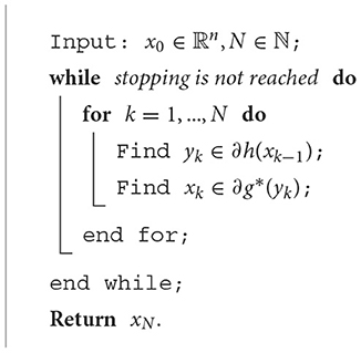
referred to as a DC optimization problem, and it can be addressed using the difference of convex algorithm introduced by Tao and An[19, 20] as follows.

The function g^* referred in the DCA is the Fenchel Conjugate of g, and it is defined as in [18]

$\begin{array}{ll}{g}^{*}(y)=sup\left\{\langle y,x\rangle -g(x)\mid x\in {ℝ}^n\right\},y\in {ℝ}^n,& (2)\end{array}$

and it is always convex regardless of whether g is convex or not.

Theorem 1. [18] Let g : ℝⁿ → (−∞, ∞] be a proper extended real-valued function, for x, y ∈ ℝⁿ. Then, x ∈ ∂g^*(y) if and only if y ∈ ∂g(x).

Definition 2. [12] A vector v ∈ ℝⁿ is a sub-gradient of a convex function f : ℝⁿ → (−∞, ∞], at $\bar{x}\in dom(f)$, if it satisfies the inequality

$f(x)\ge f(\bar{x})+\langle v,x-\bar{x}\rangle \text{ for all }x\in {ℝ}^n.$

The set of all sub-gradients of f at $\bar{x}$, denoted as $\partial f(\bar{x})$, is known as the sub-differential of f at $\bar{x}$, that is,

$\begin{array}{ll}\partial f(\bar{x})=\left\{v\in {ℝ}^n\mid f(x)\ge f(\bar{x})+\langle v,x-\bar{x}\rangle \text{ for all }x\in {ℝ}^n\right\}.& (3)\end{array}$

Theorem 2. Let $f_i:{ℝ}^n\to (-\infty ,\infty ]$ be a proper and extended real-valued convex function on ℝⁿ, where i = 1, 2, …, m and ${\bigcap }_{i=1}^{m}rint(dom(f_i))\ne \varnothing$ [12]. Then for all $\bar{x}\in {\bigcap }_{i=1}^{m}dom(f_i)$,

$\begin{array}{l}\partial \left({\displaystyle \sum _{i=1}^m}{f}_i(\bar{x})\right)={\displaystyle \sum _{i=1}^m}\partial f_i(\bar{x}).\end{array}$

2.1 The max, min, and convergence of the DCA

The maximum function is defined as the point-wise maximum of convex functions. For i = 1, 2, 3, …, m, let the functions $f_i:{ℝ}^n\to ℝ$ be closed and convex. Then, the maximum function

$f(x):={\displaystyle \underset{i=1,\dots ,m}{max}}{f}_i(x)=max\left\{f_1(x),f_2(x),\dots ,f_m(x)\right\},$

is also closed and convex. On the other hand, the minimum function f(x), defined by

$f(x):={\displaystyle \underset{i=1,\dots ,m}{min}}{f}_i(x)=min\left\{f_1(x),f_2(x),\dots ,f_m(x)\right\}$

may not be convex. However, it can always be represented as a difference of two convex functions as follows:

$\begin{array}{ll}min\left\{f_1(x),f_2(x),\dots ,f_m(x)\right\}={\displaystyle \sum _{i=1}^m}{f}_i(x)-{\displaystyle \underset{t=1,...,m}{max}}{\displaystyle \sum _{i=1,i\ne t}^m}{f}_i(x).& (4)\end{array}$

Lemma 3. [12] Let functions f_i(x), i = 1 … m be closed and convex. Then, the maximum function

$f(x)=max\left\{f_1(x),\dots ,f_m(x)\right\}$

is also closed and convex. Moreover, for any $x\in int(domf)={\cap }_{i=1}^{m}int(dom{f}_i)$, we have

$\partial f(x)=Conv\left\{\partial f_i(x)|i\in I(x)\right\},$

where I(x) = {i : f_i(x) = f(x)}.

Definition 3. [14] A function f : ℝⁿ → ℝ is ρ-strongly convex if there exists ρ > 0 such that the function

$g(x):=f(x)-\frac{\rho }{2}\left|\right|x|{|}^2$

is convex. In particular, if f is strongly convex, then f is also strictly convex, in the sense that f(λx₁ + (1 − λ)x₂) < λf(x₁) + (1 − λ)f(x₂) for all λ ∈ (0, 1).

Theorem 4. [14, 20] Let f be as defined in problem (1), and let {x_k} be a sequence generated by the DCA Algorithm 1. Suppose that g and h are ρ₁ and ρ₂ strongly convex, respectively. Then, at every iteration number k of the DCA, we have

$\begin{array}{ll}f(x_{k+1})\le f(x_k)-\frac{{\rho }_1+{\rho }_2}{2}\left|\right|x_{k+1}-x_k|{|}^2.& (5)\end{array}$

Algorithm 1

Algorithm 1. DCA algorithm 1

Moreover, if f is bounded from below and if {x_k} is bounded, then all sub-sequential limits of {x_k} converge to a stationary point of f.

2.2 Nesterov's smoothing approximation of the ℓ₁ Norm

Definition 4. [12, 14] Let F be a non-empty closed subset of ℝⁿ and let x ∈ ℝⁿ.

1. Define the distance between x and set F by

$d_F(x)=inf\left\{\left|\right|x-w\left|\right|\mid w\in F\right\}.$

2. The set of all Euclidean projection from x to F is defined by

$P(x;F)=\left\{w\in F\mid d_F(x)=\left|\right|x-w\left|\right|\right\}.$

It is well-known that P(x; F) is non-empty when F ⊂ ℝⁿ is closed. If we assume in addition that F is convex, than P(x; F) is a singleton.

Proposition 5. [11, 15] Given any a ∈ ℝⁿ and γ > 0, Nesterov's smoothing approximation of φ(x) = ||x − a||₁ has the representation

${\phi }_{\gamma }(x):=\frac{1}{2\gamma }||x-a|{|}^2-\frac{\gamma }{2}{\left[d_F\left(\frac{x-a}{\gamma }\right)\right]}^2,$

where F is the closed unit box of ℝⁿ, that is, F :$=\{x=(x^1,\dots ,x^n)\in {ℝ}^n\mid -1\le x_i\le 1\text{ for }i=1,\dots ,n\}$ for i = 1, …, n}. Moreover,

$\begin{array}{l}\nabla {\phi }_{\gamma }(x)=P\left(\frac{x-a}{\gamma };F\right)\\ =P\left(\frac{x-a}{\gamma };F\right)\\ =max(-e,min(\frac{x-a}{\gamma },e))\text{ component-wise,}& (6)\end{array}$

where P is the Euclidean projection from $\left(\frac{x-a}{\gamma }\right)$ onto unit box F, and e ∈ ℝⁿ is a vector with one in each coordinate and zero elsewhere. In addition, ${\phi }_{\gamma }(x)\le \phi (x)\le {\phi }_{\gamma }(x)+\frac{\gamma }{2}$.

3 Problems formulation

To define our problems, consider a set A of m data points, that is, A = {aⁱ ∈ Rⁿ:i = 1, …, m} and k variable cluster centers denoted by x¹, …, x^k. We model a two-level hierarchical clustering problem by choosing k separate cluster centers from which one is the headquarter that serves the centers. Other members of the data will be assigned to one of the cluster based on the ℓ₁ norm between the data points and centers. Thus, nodes are grouped into k variable centers by minimizing the ℓ₁ distances from all node to k centers. Then, a headquarter is a center that minimizes the overall distance of the network and also serves as a cluster center. Then, headquarter is defined to be mean of x^j for j = 1, .., k, that is, $\bar{x}=\frac{1}{k}\sum _{j=1}^k{x}^j$. This constraint limits the search region for headquarter to mean of selected centers or node near mean. Mathematically, the problem is defined as follows:

$\begin{array}{c}f(X)={\displaystyle \sum _{i=1}^m}min\left\{\left|\right|x^1-a^i|{|}_1,...,||x^k-a^i|{|}_1,\left|\right|\bar{x}-a^i|{|}_1\right\}\\ +{\displaystyle \sum _{j=1}^k}\left|\right|x^j-\bar{x}|{|}_1\end{array}$

is minimized, where,

$\bar{x}=\frac{1}{k}{\displaystyle \sum _{j=1}^k}{x}^j$

In addition, to insure the centers are real node, the points $\bar{x},x^1,x^2,...,x^k$ should satisfy the following condition:

${\displaystyle \underset{i=1,...,m}{min}}\left|\right|\bar{x}-a^i|{|}_1+{\displaystyle \sum _{j=1}^k}{\displaystyle \underset{i=1,...m}{min}}||x^j-a^i|{|}_1=0$

Thus, the problem is formulated as

$\begin{array}{ll}\text{minimize}\left\{{\displaystyle \sum _{i=1}^m}{\displaystyle \underset{j=1,...,k+1}{min}}\left|\right|x^j-a^i|{|}_1+{\displaystyle \sum _{j=1}^k}||x^j-\bar{x}|{|}_1\right\}& (7)\end{array}$

subject to

$\begin{array}{ll}{\displaystyle \sum _{j=1}^{k+1}}{\displaystyle \underset{i=1,...m}{min}}\left|\right|x^j-a^i|{|}_1=0,& (8)\end{array}$

where x^k+1 in the summation is $\bar{x}$. The constraints in (8) are used to force the centers to lie on real node and to force headquarter to be on or near mean of the centers based on minimum distance.

We can write (7) as unconstrained problem using penalty parameter τ > 0, as follows:

$\begin{array}{l}\text{minimize}({\displaystyle \sum _{i=1}^m{\min }_{j=1,\mathrm{...},k+1}}\Vert x^j-a^i{\Vert }_1+{\displaystyle \sum _{j=1}^k\Vert x^j-\overline{x}{\Vert }_1}\\ +\tau {\displaystyle \sum _{i=1}^{k+1}{\min }_{i=1,\mathrm{...},m}}\Vert x^j-a^i{\Vert }_1).\end{array}$

Writing (9) as the sum and maximum of convex functions using the formula in (4) as follows:

$\begin{array}{c}f(X)={\displaystyle {\sum }_{i=1}^m}{\displaystyle {\sum }_{j=1}^{k+1}}\left|\right|x^j-a^i|{|}_1\\ -{\displaystyle {\sum }_{i=1}^m}{\displaystyle {max}_{t=1,...,k+1}}{\displaystyle {\sum }_{j=1,j\ne t}^{k+1}}\left|\right|x^j-a^i|{|}_1+{\displaystyle {\sum }_{j=1}^k}||x^j-\bar{x}|{|}_1\\ +\tau {\displaystyle {\sum }_{i=1}^m}{\displaystyle {\sum }_{j=1}^{k+1}}\left|\right|x^j-a^i|{|}_1-\tau {\displaystyle {max}_{t=1,...,k+1}}\\ {\displaystyle {\sum }_{j=1,j\ne t}^{k+1}}\left|\right|x^j-a^i|{|}_1.& (9)\end{array}$

Expressing (9) as DC function, we have

$\begin{array}{l}f(X)=(1+\tau ){\displaystyle \sum _{i=1}^m}{\displaystyle \sum _{j=1}^{k+1}}\left|\right|x^j-a^i|{|}_1+{\displaystyle \sum _{j=1}^k}||x^j-\bar{x}|{|}_1\\ -{\displaystyle \sum _{i=1}^m}{\displaystyle \underset{t=1,...,k+1}{max}}{\displaystyle \sum _{j=1,j\ne t}^{k+1}}\left|\right|x^j-a^i|{|}_1\\ -\tau {\displaystyle \sum _{j=1}^{k+1}}{\displaystyle \underset{r=1,...,m}{max}}{\displaystyle \sum _{i=1,i\ne r}^m}\left|\right|x^j-a^i|{|}_1,& (10)\end{array}$

where

$\begin{array}{l}g(X)=(1+\tau ){\displaystyle \sum _{i=1}^m}{\displaystyle \sum _{j=1}^{k+1}}\left|\right|x^j-a^i|{|}_1+{\displaystyle \sum _{j=1}^k}||x^j-\bar{x}|{|}_1,\text{ and}\end{array}$

$\begin{array}{l}h(X)={\displaystyle \sum _{i=1}^m}{\displaystyle \underset{t=1,...,k+1}{max}}{\displaystyle \sum _{j=1,j\ne t}^{k+1}}\left|\right|x^j-a^i|{|}_1\\ +\tau {\displaystyle \sum _{j=1}^{k+1}}{\displaystyle \underset{r=1,...,m}{max}}{\displaystyle \sum _{i=1,i\ne r}^m}\left|\right|x^j-a^i|{|}_1.& (11)\end{array}$

Since f is DC function based on Proposition 5 and ℓ₁ smoothing studied in [11], we obtain a Nesterov's approximation of ||x − a||₁ as

$\left|\right|x-a|{|}_1:=\frac{\gamma }{2}\left[||\frac{x-a}{\gamma }|{|}^2-{\left[d_F(\frac{x-a}{\gamma })\right]}^2\right].$

The main goal is to minimize the partially smoothed objective given by,

$\begin{array}{l}{f}_{\gamma }(X)=\frac{(1+\tau )\gamma }{2}{\displaystyle \sum _{i=1}^m}{\displaystyle \sum _{j=1}^{k+1}}\left|\right|\frac{x^j-a^i}{\gamma }|{|}^2+{\displaystyle \sum _{j=1}^k}|\left|\frac{x^j-\bar{x}}{\gamma }\right|{|}^2\\ -\frac{(1+\tau )\gamma }{2}{\displaystyle \sum _{i=1}^m}{\displaystyle \sum _{j=1}^{k+1}}{\left[d_F(\frac{x^j-a^i}{\gamma })\right]}^2-\frac{\gamma }{2}{\displaystyle \sum _{j=1}^k}{\left[d_F(\frac{x^j-\bar{x}}{\gamma })\right]}^2\\ -{\displaystyle \sum _{i=1}^m}{\displaystyle \underset{t=1,...,k+1}{max}}{\displaystyle \sum _{j=1,j\ne t}^{k+1}}\left|\right|x^j-a^i|{|}_1& (12)\end{array}$

$\begin{array}{l}-\tau {\displaystyle \sum _{j=1}^{k+1}}{\displaystyle \underset{r=1,...,m}{max}}{\displaystyle \sum _{i=1,i\ne r}^m}\left|\right|x^j-a^i|{|}_1.\end{array}$

That is $\mathrm{\text{minimize}}\left\{f_{\gamma }(X)=g_{\gamma }(X)-h_{\gamma }(X)\right\},X\in {ℝ}^{k\times n}.$

In addition, g_γ is the sum of convex functions defined as

$\begin{array}{ll}{g}_{\gamma }(X)=g_{1\gamma }(X)+g_{2\gamma }(X)& (13)\end{array}$

where

$\begin{array}{l}{g}_{1\gamma }(X)=\frac{(1+\tau )\gamma }{2}{\displaystyle \sum _{i=1}^m}{\displaystyle \sum _{j=1}^{k+1}}\left|\right|\frac{x^j-a^i}{\gamma }|{|}^2,g_{2\gamma }(X)={\displaystyle \sum _{j=1}^k}|\left|\frac{x^j-\bar{x}}{\gamma }\right|{|}^2.\end{array}$

And h_γ is also the sum of four convex functions defined as

$\begin{array}{ll}{h}_{\gamma }(X)=h_{1\gamma }(X)+h_{2\gamma }(X)+h_{3\gamma }(X)+h_{4\gamma }(X),& (14)\end{array}$

where

$\begin{array}{l}{h}_{1\gamma }(X)=\frac{(1+\tau )\gamma }{2}{\displaystyle \sum _{i=1}^m}{\displaystyle \sum _{j=1}^{k+1}}{\left[d_F(\frac{x^j-a^i}{\gamma })\right]}^2\\ h_{2\gamma }(X)=\frac{\gamma }{2}{\displaystyle \sum _{j=1}^k}{\left[d_F(\frac{x^j-\bar{x}}{\gamma })\right]}^2,\\ h_{3\gamma }(X)={\displaystyle \sum _{i=1}^m}{\displaystyle \underset{t=1,...,k+1}{max}}{\displaystyle \sum _{j=1,j\ne t}^{k+1}}\left|\right|x^j-a^i|{|}_1,\\ h_{4\gamma }(X)=\tau {\displaystyle \sum _{j=1}^{k+1}}{\displaystyle \underset{r=1,...,m}{max}}{\displaystyle \sum _{i=1,i\ne r}^m}\left|\right|x^j-a^i|{|}_1.\end{array}$

For the calculation of gradient and sub-gradient, consider a data matrix A with aⁱ, i = 1, ..., m, in the i^th row and a variable matrix X with x^j,j = 1, 2, ..., k + 1 in the j^th row.

Since X and A belongs to a linear space of real matrices, we can apply inner product such that

$\langle X,A\rangle =\text{trace}(X^{T}A)={\displaystyle \sum _{i=1}^n}{\displaystyle \sum _{j=1}^k}{x}_{ij}{a}_{ij}.$

And the Frobenius norm on ℝ^k×m is given by

$\begin{array}{ll}\left|\right|A|{|}_F=\sqrt{\langle A,A\rangle }=\sqrt{{\displaystyle \sum _{j=1}^k}\langle a^j,a^j\rangle }=\sqrt{{\displaystyle \sum _{j=1}^k}||a^j|{|}^2}.& (15)\end{array}$

To calculate the gradient of g_γ in (13), let X be of size (k + 1) × n is variable matrix. Then,

$\begin{array}{l}{g}_{1\gamma }(X):=\frac{(1+\tau )}{2\gamma }{\displaystyle \sum _{i=1}^m}{\displaystyle \sum _{j=1}^{k+1}}\left|\right|x^j-a^i|{|}^2,\\ =\frac{(1+\tau )}{2\gamma }{\displaystyle \sum _{i=1}^m}{\displaystyle \sum _{j=1}^k}\left[\left|\right|x^j|{|}^2-2\langle x^j,a^i\rangle +|\left|a^i\right|{|}^2\right],\\ =\frac{(1+\tau )}{2\gamma }\left[m\left|\right|X|{|}_F^2-2\langle X,E_{km}A\rangle +k|\left|A\right|{|}_F^2\right],\end{array}$

where $E_{km}\in {ℝ}^{k+1\times m}$ is a matrix of all ones. As g_1γ is smooth, then

${\nabla }_x{g}_{1\gamma }(X)=\frac{(1+\tau )}{\gamma }\left[mX-B\right],\text{ where }B=E_{km}A.$

Again consider g_2γ which is differentiable function,

$\begin{array}{l}{g}_{2\gamma }(X):=\frac{1}{2\gamma }{\displaystyle \sum _{j=1}^k}||x^j-\bar{x}|{|}^2,\\ =\frac{1}{2\gamma }{\displaystyle \sum _{j=1}^k}\left[||x^j|{|}^2-2\langle x^j,\bar{x}\rangle +\langle x^j,\bar{x}\rangle \right],\\ =\frac{1}{2\gamma }\left[||X|{|}_F^2-\frac{2}{k}\langle X,E_{kk}X\rangle +\frac{1}{k}\langle X,E_{kk}X\rangle \right],\end{array}$

where E_kk is a k × k matrix with elements all ones. Then, the gradients of g_2γ are given by

$\begin{array}{l}{\nabla }_x{g}_{2\gamma }(X)=\frac{1}{\gamma }\left[X-\frac{1}{k}{E}_{kk}X\right],\\ =\frac{1}{\gamma }\left[X-HX\right],\text{ where }H=\frac{1}{k}{E}_{kk}.\end{array}$

Next, we focus on X ∈ ∂g^*(Y) where g^* is a Fenchel conjugate defined in (2) and can be calculated using the fact that X ∈ ∂g^*(Y)⇔Y ∈ ∂g(X). Since g_γ is differentiable. Thus,

$\begin{array}{l}{\nabla }_x{g}_{\gamma }(X)={\nabla }_x{g}_{1\gamma }(X)+{\nabla }_x{g}_{2\gamma }(X),\\ Y=\frac{(1+\tau )}{\gamma }\left[mX-B\right]+\frac{1}{\gamma }\left[X-HX\right],\\ =\left[\frac{(1+\tau )}{\gamma }m+\frac{1}{\gamma }\left[\mathbb{I}-H\right]\right]X-\left[\frac{(1+\tau )}{\gamma }B\right],\\ =\frac{1}{\gamma }\left[(1+\tau )m+\mathbb{I}-H\right]X-\left[\frac{(1+\tau )}{\gamma }B\right],\\ =\frac{1}{\gamma }\left[(1+\tau )m+1]\mathbb{I}-H\right]X-\left[\frac{(1+\tau )}{\gamma }B\right],\\ =\frac{1}{\gamma }\left[a\mathbb{I}-bH\right]X-\left[\frac{(1+\tau )}{\gamma }B\right],\end{array}$

where a = (1 + τ)m + 1 and b = 1.

Let N = a𝕀 − bH, then N is invertible as N⁻¹ = α𝕀 + βH where

$\begin{array}{r}\alpha =\frac{1}{a}=\frac{1}{(1+\tau )m+1}\text{ and }\\ \beta =\frac{b}{a\left[a+bk\right]}=\frac{1}{(1+\tau )m+1\left[(1+\tau )m+1+k\right]},\end{array}$

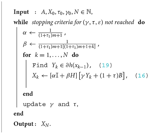
(see Lemma 5.1 of [8]). Therefore,

$\begin{array}{ll}X=\left[\alpha \mathbb{I}-\beta H\right]\left[\gamma Y_x+(1+\tau )B\right].& (16)\end{array}$

Next, we find the sub-gradient in (14) and this can be done by search Y ∈ ∂h_γ(X). Given a smooth functions h_1γ and h_2γ, the partial gradient at x^j for j = 1, …, k + 1 is

$\begin{array}{c}{h}_{1\gamma }=\frac{(1+\tau )\gamma }{2}{\displaystyle \sum _{i=1}^m}{\displaystyle \sum _{j=1}^{k+1}}{\left[d_F(\frac{x^j-a^i}{\gamma })\right]}^2\\ \frac{\partial h_{1\gamma }}{\partial x^j}(X)=(1+\tau )\gamma {\displaystyle \sum _{i=1}^m}\left[\frac{x^j-a^i}{\gamma }-P(\frac{x^j-a^i}{\gamma };F)\right].& (17)\end{array}$

Thus, ∇h_1γ(X)) is a matrix with dimension (k + 1) × n with j^th row is $\frac{\partial h_{1\gamma }}{\partial x^j}(X)$.

The gradients of $h_{2\gamma }=\frac{\gamma }{2}\sum _{j=1}^k{\left[d_F(\frac{x^j-\bar{x}}{\gamma })\right]}^2$ at X are given by

$\begin{array}{l}\frac{\partial h_{2\gamma }}{\partial x^j}(X)=\frac{x^j-\bar{x}}{\gamma }-P(\frac{x^j-\bar{x}}{\gamma };F)\\ -\frac{1}{k}{\displaystyle \sum _{\ell =1}^k}\left[\frac{x^{\ell }-\bar{x}}{\gamma }-P(\frac{x^{\ell }-\bar{x}}{\gamma };F)\right].& (18)\end{array}$

The projections in (17) and (18) are the Euclidean projection from v ∈ ℝⁿ onto a unit closed box F which are defined as

$P(v,F)=max(-e,min(v,e)).$

where e ∈ ℝⁿ is a vector with one in each coordinate and zero elsewhere.

Since we use ℓ₁ norm, next we illustrate how to find the sub-gradient Y ∈ ∂h_γ(X) for the case where F is the closed unit box in ℝⁿ.

For a given x ∈ ℝ, we define

$\text{sign(}x\text{)}:=\{\begin{array}{c}\begin{array}{ccc}1& if& x>0,\\ 0& if& x=0,\\ -1& if& x<0.\end{array}\end{array}$

Then, we define sign(x): = (sign(x₁), …, sign(x_n)) for $x=(x_1,\dots ,x_n)\in {ℝ}^n.$ Note that the sub-gradients of f(x) = ||x||₁ at x ∈ ℝⁿ are s_i = sign(x) if x_i ≠ 0 and s_i ∈ [−1, 1] if x_i = 0.

The sub-gradients of the non-smooth functions h_3γ and h_4γ are calculated as the sub-differential of point-wise maximum functions,

$\begin{array}{l}{h}_{3\gamma }:={\displaystyle \sum _{i=1}^m}{\displaystyle \underset{r=1,\dots ,k}{max}}{\displaystyle \sum _{j=1,j\ne r}^k}\left|\right|x^j-a^i|{|}_1={\displaystyle \sum _{i=1}^m}{\varphi }_i(\text{X}),\end{array}$

where, for i = 1, …, m,

${\varphi }_i(\text{X}):=max\left\{{\varphi }_{ir}(\text{X})={\displaystyle \sum _{j=1,j\ne r}^k}||x^j-a^i|{|}_1,r=1,\dots ,k\right\}.$

To do this, for each i = 1, …, m, we first find U_i ∈ ∂ϕ_i(X) according to Lemma 3. Then, we define $\text{U}:=\sum _{i=1}^m{\text{U}}_i$ to get a sub-gradient of the function h_3γ at X by the sub-differential sum rule. To accomplish this goal, we first choose an index r^* from the index set {1, …, k} such that

${\varphi }_i(\text{X})={\varphi }_{i{r}^{*}}(\text{X})={\displaystyle \sum _{j=1,j\ne r^{*}}^k}||x^j-a^i|{|}_1.$

Using the familiar sub-differential formula of the ℓ₁ norm function, the j^th row $u_i^j$ for j ≠ r^* of the matrix U_i is determined as follows:

$\begin{array}{l}{u}_i^j:=\text{sign}(x^j-a^i)=\{\begin{array}{cc}1& \text{if }{x}^j>a^i,\\ 0& \text{if }{x}^j=a^i,\\ -1& \text{if }{x}^j<a^i.\end{array}\end{array}$

The r^*th row of the matrix U_i is $u_i^{r^{*}}:=0$.

Similarly, the sub-gradient of h_4γ is given by

$\begin{array}{ll}{h}_{4\gamma }& :=\tau {\displaystyle \sum _{j=1}^k}{\displaystyle \underset{s=1,...,m}{max}}{\displaystyle \sum _{i=1,i\ne s}^m}||x^j-a^i|{|}_1=\tau {\displaystyle \sum _{j=1}^k}{\psi }_j(\text{X}),\end{array}$

where, for j = 1, …, k,

${\psi }_j(\text{X}):=max\left\{{\psi }_{js}(\text{X})={\displaystyle \sum _{i=1,i\ne s}^m}||x^j-a^i|{|}_1,s=1,\dots ,m\right\}.$

To do this, for each j = 1, …, k, we first find W_j ∈ ∂ψ_j(X). Then, we define $\text{W}:=\tau \sum _{j=1}^k{\text{W}}_j$ to get a sub-gradient of the function h_4γ at X by the sub-differential sum rule. To accomplish this goal, we first choose an index s^* from the index set {1, …, m} such that

${\psi }_j(\text{X})={\psi }_{j{s}^{*}}(\text{X})={\displaystyle \sum _{j=1,j\ne s^{*}}^k}||x^j-a^i|{|}_1.$

The s^*th row of the matrix W_j is $w_{s^{*}}^j:=0$.

Thus, the sub-gradient of h_4γ is defined as

$\frac{\partial h_{4\gamma }}{\partial x^j}:=\tau \text{W}.$

From the sub-gradient calculated above we have,

$\begin{array}{ll}Y=\frac{\partial h_{1\gamma }}{\partial x^j}(X)+\frac{\partial h_{2\gamma }}{\partial x^j}(X)+\frac{\partial h_{3\gamma }}{\partial x^j}(X)+\frac{\partial h_{4\gamma }}{\partial x^j}(X)& (19)\end{array}$

Now, we have in position to implement DCA algorithm that will solve the problem as shown in DCA Algorithm 2.

Algorithm 2

Algorithm 2. Bi-level hierarchical clustering.

4 Simulation results

The numerical simulation was performed on an HP laptop with an Intel(R) Core(TM) i7-8565U at 1.80 GHz 1.99 GHz processor, 8.00 GB RAM with MATLAB version R2017b. Various parameters were used during the simulation, among others we used a large increasing penalty parameter τ and a decay smoothing parameter γ. These parameters are updated during iteration as in [6]; τ_i+1 = σ₁τ_i, σ₁ > 1 and γ_i+1 = σ₂γ_i, 0 < σ₂ < 1 and ϵ = 1e − 6. We chose the initial penalty parameter (${\tau }_0=e^{-6}$) and the initial smoothing parameter γ₀ = 1. In addition, after varying the parameters, we chose ${\sigma }_1\le 16e^9$ as the growth factor of the penalty parameter, σ₂ = 0.5 the decrease factor of the smoothing parameter, and the stopping criterion $\frac{\left|\right|X_{k+1}-X_k|{|}_F}{\left|\right|X_k|{|}_F+1}\le ϵ$ for inner for loop. To implement the algorithms, we used randomly selected default cluster centers from the datasets.

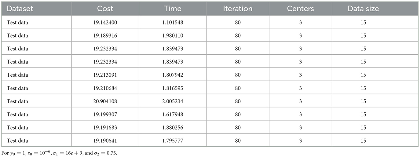
The performance of the DCA Algorithm 2 was tested with different datasets. We first tested the algorithm on a small dataset taken from [8], and the result shows that it converges to the same cluster centers as in [8] with a different objective value due to the ℓ₁ norm. Since the ℓ₁ distance is greater than or equal to the Euclidean distance, it depends on the data points. As shown in Table 1, the algorithm converges to the optimal point approximately 85.71%. This means that out of 7 iterations, 6 of them converge to the same objective valve.

Table 1

Table 1. Ten iterations for the 15 point test dataset.

Second, we tested the proposed algorithm with EIL76 (The 76 City Problem) datasets taken from [7] with four clusters, one of which serves as HQ, which converge to near-optimal cluster centers in a reasonable time compared to study [8, 13] (see Figure 1).

Figure 1

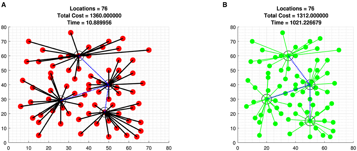
Figure 1. Optimal cost of EIL76 (The 76 City Problem) data taken from [7] with four clusters one serves as HQ. (A) A EIL76 data with Algorithm 2. (B) A EIL76 data with brute-force iteration.

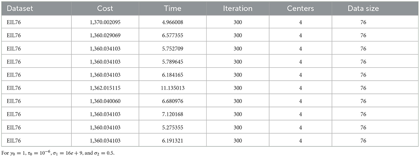
It is also observed in the EIL76 (The 76 City Problem) data which converge to the same or close cluster centers with higher objective cost, fewer iterations, and almost the same time compared to the study of [8] iterated using MATLAB (see Table 2).

Table 2

Table 2. Ten iterations for EIL76 dataset.

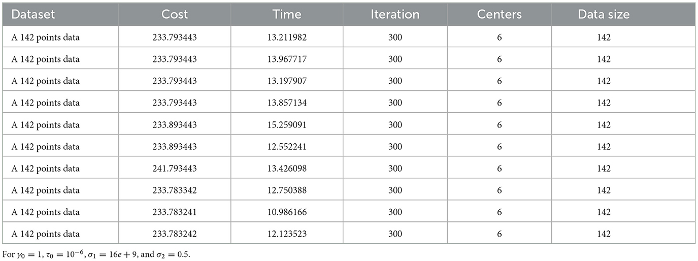
Third, we applied our proposed algorithm to a GPS data from 142 cities and towns in Ethiopia with more than 7,000 inhabitants, including 65 in Oromia regional state. We tested the algorithm with 65 nodes, 4 cluster centers, one of which serves as HQ, and 142 nodes with six clusters (see Figures 2, 3), which converge 86% to the optimal solution. This means that out of 7 iterations, 6 of them converge to the near-optimal values shown in Tables 3, 4.

Figure 2

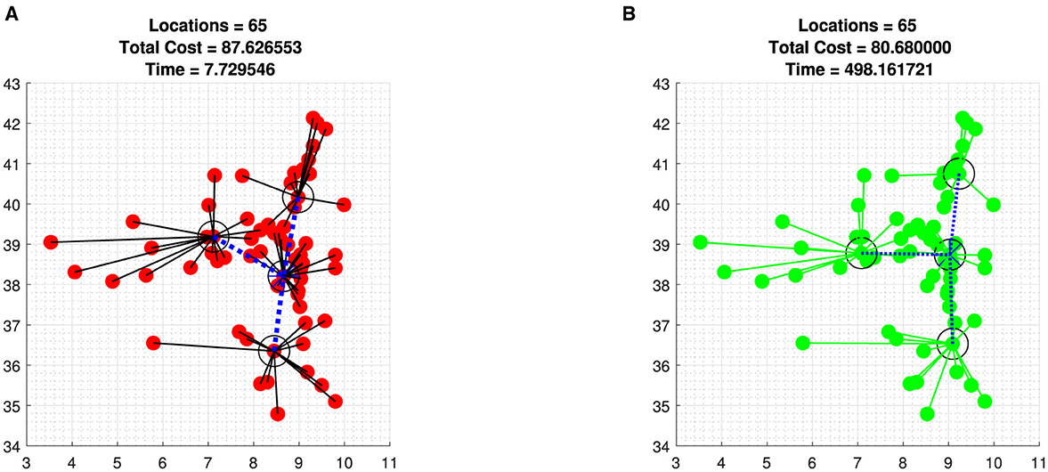
Figure 2. Datasets of 65 Oromia regional cities and towns with four clusters one serves as HQ. (A) Sixty-five data points using Algorithm 2. (B) Sixty-five data points with brute-force iteration.

Figure 3

Figure 3. Datasets of 142 Ethiopian towns and cities with six clusters one serves as HQ. (A) Beginning of iterations. (B) Few iterations. (C) Optimal iterations.

Table 3

Table 3. Ten iterations for the 65 point test dataset.

Table 4

Table 4. Ten iterations for the 142 point test dataset.

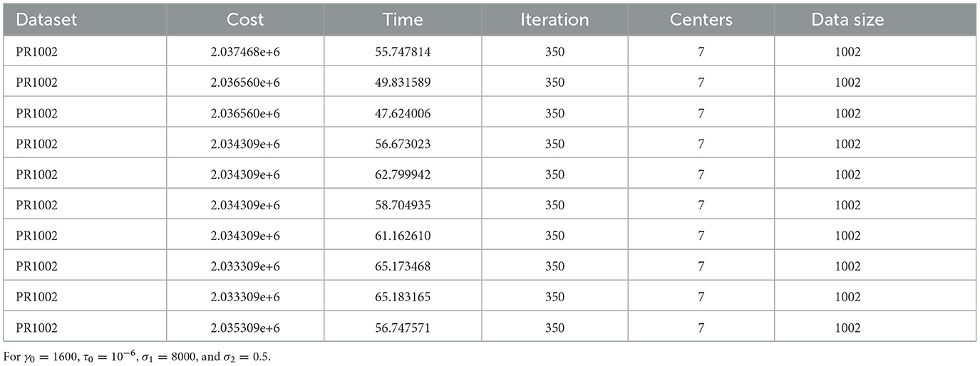
Fourth, we tested the proposed algorithm with PR1002 (The 1002 City Problem) datasets taken from [7] with seven clusters, one of which serves as HQ, which converge to near-optimal cluster centers in a reasonable time compared to study [8, 13] (see Table 5 and Figure 4).

Table 5

Table 5. Ten iterations for PR1002 dataset.

Figure 4

Figure 4. Datasets of PR1002 (The 1002 City Problem) taken from [7] with seven clusters and one serving as HQ. (A) Beginning of iteration. (B) Few iteration. (C) Optimal iteration.

To show how the objective functions improved with iteration, we include a plot of the first few iterations of Figures 3, 4, which shows the dynamics of the algorithm (see Figures 3A, B, 4A, B).

In general, since the algorithm is a modified DCA and DCA is a local search algorithm, there is no guarantee that our algorithms converge to the global optimal solution. However, we compared our result with ℓ₂ norm in [8, 13], and it shows that our proposed algorithm converges with fewer iteration but relatively the same computational time for data iterated with MATLAB in [8]. In addition, we compared our result with brute-force generated solutions for datasets with fewer nodes (see Figures 1A, B, 2A, B) which converge to a near-optimal value with reasonable time compared to the brute-force iterations.

We expect that our method used in this study to solve the two-level clustering problem with the ℓ₁ norm is less sensitive to outliers compared to the ℓ₂ norm, which minimizes possible clustering errors. In addition, it can be used to solve other non-smooth and non-convex optimization problems in signal processing, such as image pixel clustering for image segmentation and compressed sensing.

For the following tables, we conducted an experiment with fixed iteration numbers for each dataset and initial cluster centers were randomly selected from the datasets. The cost is obtained by minimizing Equation (7).

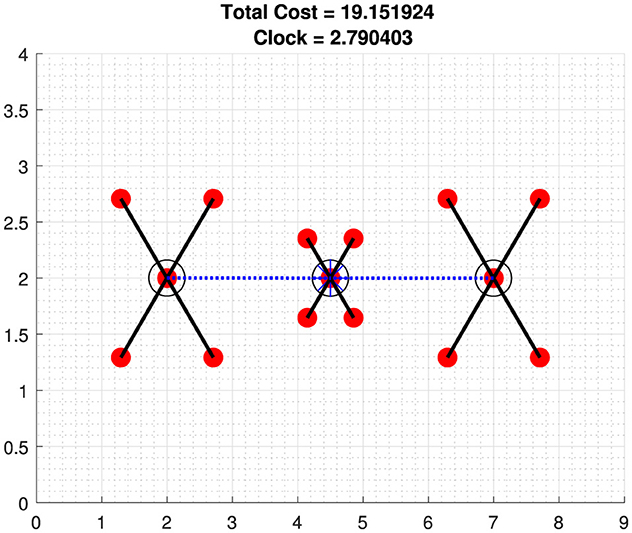
Figure 5 shows the optimal cost of test data taken from [8] with optimal clusters centers and HQ,

$\begin{array}{c}X=\left(\begin{array}{cc}7.0000& 2.0000\\ 4.5000& 2.0000\\ 2.0000& 2.0000\end{array}\right),HQ=(4.50002.0000)\end{array}$

Figure 5

Figure 5. Fifteen point test dataset with three clusters and one serves as HQ.

In Figure 1 the selected cluster centers and HQ are

$\begin{array}{c}X=\left(\begin{array}{cc}26.0000& 29.0000\\ 35.0000& 60.0000\\ 50.0000& 40.0000\\ 48.0000& 21.0000\end{array}\right)HQ=(50.000040.0000),\end{array}$

In Figure 2 the selected cluster centers and HQ are

$\begin{array}{c}X=\left(\begin{array}{cc}8.4500& 36.3500\\ 8.8990& 39.9171\\ 8.6607& 38.2124\\ 6.6100& 38.4200\end{array}\right)\text{ and }HQ=(8.660738.2124).\end{array}$

In Figure 3 the selected cluster centers and HQ are

$\begin{array}{c}X=\left(\begin{array}{cc}10.3400& 37.7199\\ 8.4500& 36.3500\\ 6.9595& 39.1795\\ 8.9131& 38.6186\\ 8.9808& 40.1709\\ 12.0400& 39.0400\end{array}\right)\text{ and }HQ=(8.915638.6189).\end{array}$

For this particular dataset, we used γ₀ = 1600 and σ₁ = 8000. In Figure 4 the selected cluster centers and HQ are

$\begin{array}{c}X=\left(\begin{array}{cc}5218.0000& 4090.0000\\ 5923.0000& 9557.0000\\ 1083.9000& 9857.0000\\ 1473.5000& 4145.0000\\ 9977.0000& 3008.0000\\ 1547.1000& 9522.0000\\ 9892.0000& 6023.0000\end{array}\right)\text{ and }HQ=(9891.60006023.0000).\end{array}$

5 Conclusion

In this study, we used a continuous formulation of discrete two-level hierarchical clustering, where the distance between two data points is measured by the ℓ₁ norm. As a result, it became non-smooth and non-convex, on which Nesterov's smoothing and DC-based algorithms were implemented. We observe that parameter selection is the decisive factor in terms of accuracy and speed of convergence of our proposed algorithms. The performance of Algorithm 2 highly depends on the initial values set to the penalty and smoothing parameter.

The algorithm was tested with real and known source datasets of different sizes in MATLAB. Starting from different random initial cluster centers, the algorithm converges to a near-optimal value in a reasonable time. As a result, improved iteration time for large-scale problems and convergence to a near-optimal solution were observed.

Data availability statement

The original contributions presented in the study are included in the article/Supplementary material, further inquiries can be directed to the corresponding author.

Author contributions

AG: Investigation, Software, Writing – original draft, Conceptualization, Data curation, Formal analysis, Funding acquisition, Methodology, Project administration, Resources, Supervision, Validation, Visualization, Writing – review & editing. LO: Conceptualization, Formal analysis, Supervision, Validation, Writing – review & editing.

Funding

The author(s) declare that no financial support was received for the research, authorship, and/or publication of this article.

Acknowledgments

Authors are grateful to the referees and handling editor for their constructive comments.

Conflict of interest

The authors declare that the research was conducted in the absence of any commercial or financial relationships that could be construed as a potential conflict of interest.

Publisher's note

All claims expressed in this article are solely those of the authors and do not necessarily represent those of their affiliated organizations, or those of the publisher, the editors and the reviewers. Any product that may be evaluated in this article, or claim that may be made by its manufacturer, is not guaranteed or endorsed by the publisher.

Supplementary material

The Supplementary Material for this article can be found online at: https://www.frontiersin.org/articles/10.3389/fams.2024.1445390/full#supplementary-material

References

1. An LTH, Belghiti MT, Tao PD. A new efficient algorithm based on DC programming and DCA for clustering. J Global Optimizat. (2007) 37:593–608. doi: 10.1007/s10898-006-9066-4

Crossref Full Text | Google Scholar

2. Bagirov AM, Taheri S, Ugon J. Nonsmooth DC programming approach to the minimum sum-of-squares clustering problems. Pattern Recognit. (2016) 53:12–24. doi: 10.1016/j.patcog.2015.11.011

Crossref Full Text | Google Scholar

3. Bagirov A. Derivative-free methods for unconstrained nonsmooth optimization and its numerical analysis. Investigacao Operacional. (1999) 19:75–93.

Google Scholar

4. Bajaj A, Mordukhovich BS, Nam NM, Tran T. Solving a continuous multifacility location problem by DC algorithms. Optimizat Meth Softw. (2022) 37:338–60. doi: 10.1080/10556788.2020.1771335

Crossref Full Text | Google Scholar

5. Barbosa GV, Villas-Boas SB, Xavier AE. Solving the two-level clustering problem by hyperbolic smoothing approach, and design of multicast networks. In: The 13th World Conference on Transportation Research was organized on July 15–18, 2013 by COPPE - Federal University of Rio de Janeiro, Brazil. WCTR RIO (2013).

Google Scholar

6. Fita A, Geremew W, Lemecha L. A DC optimization approach for constrained clustering with l1-norm. Palest J Mathem. (2022) 11:3.

Google Scholar

7. Reinelt G. TSPLIB: A traveling salesman problem library. ORSA J Comp. (1991) 3:376–84. doi: 10.1287/ijoc.3.4.376

PubMed Abstract | Crossref Full Text | Google Scholar

8. Geremew W, Nam NM, Semenov A, Bogniski V, Psailio E. A DC programming approach for solving multicast network design problems via the Nesterov smoothing technique. J Global Optimizat. (2018) 72:705–29. doi: 10.1007/s10898-018-0671-9

Crossref Full Text | Google Scholar

9. Jia L, Bagirov A, Ouveysi I, Rubinov M. Optimization based clustering algorithms in Multicast group hierarchies. In: Proceedings of the Australian Telecommunications, Networks and Applications Conference (ATNAC) (2003).

Google Scholar

10. Le Thi HA, Pham Dinh T. DC programming and DCA: thirty years of developments. Mathemat Program. (2018) 169:5–68. doi: 10.1007/s10107-018-1235-y

Crossref Full Text | Google Scholar

11. Mau Nam N, Hoai An LT, Giles D, An NT. Smoothing techniques and difference of convex functions algorithms for image reconstructions. Optimization. (2020) 69:1601–33. doi: 10.1080/02331934.2019.1648467

Crossref Full Text | Google Scholar

12. Mordukhovich BS, Nam NM. An Easy Path to Convex Analysis and Applications. Cham: Springer. (2014).

Google Scholar

13. Nam NM, Geremew W, Reynolds S, Tran T. Nesterov's smoothing technique and minimizing differences of convex functions for hierarchical clustering. Optimizat Lett. (2018) 12:455–73. doi: 10.1007/s11590-017-1183-0

Crossref Full Text | Google Scholar

14. Nam NM, Rector RB, Giles D. Minimizing differences of convex functions with applications to facility location and clustering. J Optim Theory Appl. (2017) 173:255–78. doi: 10.1007/s10957-017-1075-6

Crossref Full Text | Google Scholar

15. Nesterov Y. Smooth minimization of non-smooth functions. Mathem Program. (2005) 103:127–52. doi: 10.1007/s10107-004-0552-5

Crossref Full Text | Google Scholar

16. Nesterov Y. Lectures on Convex Optimization. Cham: Springer. (2018). doi: 10.1007/978-3-319-91578-4

Crossref Full Text | Google Scholar

17. Nguyen PA, Le Thi HA. DCA approaches for simultaneous wireless information power transfer in MISO secrecy channel. Optimizat Eng. (2023) 24:5–29. doi: 10.1007/s11081-020-09570-3

Crossref Full Text | Google Scholar

18. Rockafellar R. Convex Analysis. Princeton: Princeton University Press (1970).

Google Scholar

19. Tao PD, An LTH. A DC optimization algorithm for solving the trust-region subproblem. SIAM J Optimizat. (1998) 8:476–505. doi: 10.1137/S1052623494274313

Crossref Full Text | Google Scholar

20. Tao PD, An LH. Convex analysis approach to DC programming: theory, algorithms and applications. Acta Mathematica Vietnamica. (1997) 22:289–355.

PubMed Abstract | Google Scholar

21. An LTH, Minh LH, Tao PD. Optimization based DC programming and DCA for hierarchical clustering. Eur J Operation Res. (2007) 183:1067–85. doi: 10.1016/j.ejor.2005.07.028

Crossref Full Text | Google Scholar

22. An LTH, Minh LH, Tao PD. New and efficient DCA based algorithms for minimum sum-of-squares clustering. Pattern Recogn. (2014) 47:388–401. doi: 10.1016/j.patcog.2013.07.012

Crossref Full Text | Google Scholar