Optimal control strategies for HIV and COVID-19 co-infection: a cost-effectiveness analysis

In the face of ongoing challenges posed by the COVID-19 and the persistent threat of human immunodeficiency virus (HIV), the emergence of co-infections such as COVID-19 and HIV has heightened complexities in disease management. This study aims to identify effective control strategies to mitigate COVID-19 and HIV co-infection, which aggravates the existing challenges posed by these two diseases. To achieve this, we formulated a co-infection model that describes the transmission dynamics of COVID-19 and HIV. Under certain circumstances, we established that HIV infection may facilitate COVID-19 transmission, highlighting the need to identify and implement effective interventions to mitigate COVID-19 and HIV co-infection. As a result, we incorporated four time-dependent control strategies in the co-infection model: HIV prevention, HIV treatment, COVID-19 vaccination, and COVID-19 treatment. Numerical simulations were conducted to support and clarify the analytical results and to show how preventative efforts affect the co-infected population. Simulations confirm that applying any of the study's strategies will reduce the number of co-infection cases. However, the implementation of these strategies is constrained by limited resources. Therefore, a comprehensive cost-effectiveness analysis was conducted to identify the most economically viable strategy. The analysis concludes that implementing a combined approach of vaccination and treatment for COVID-19 emerges as the most cost-effective measure for preventing the spread of COVID-19 and HIV. These findings provide crucial guidance for decision-makers in adopting precise preventive strategies, ultimately aiming to reduce mortality rates among HIV patients.

1 Introduction

The COVID-19 pandemic is the latest phenomenon that has profoundly impacted the world's social, economic, and political activities. Although we are now in the endemic phase, the effects of the disease are still ongoing. As of 12 May 2024, there have been ~7 million deaths out of 775,431,269 million infected people, and there are still millions of active COVID-19 cases [1]. Furthermore, an estimated 39 million individuals worldwide were predicted to have lived with human immunodeficiency virus (HIV)/acquired immune deficiency syndrome (AIDS) in 2022, and 1.3 million new cases were reported [2]. This situation then leads us to a co-infection of COVID-19 and HIV. The presence of HIV infection has been established as a variable that plays a role in the development of severe and critical conditions of COVID-19, as well as in the increased rates of mortality [3, 4]. HIV targets CD4+ cells, which play a crucial role in defending the body against infections. This leaves the host more susceptible to other diseases, including COVID-19. The persistence of COVID-19 poses an additional challenge, especially for patients with low CD4+ counts. Studies are showing that such eye patients are more likely to suffer serious health problems from COVID-19 [5–8].

The human immunodeficiency virus (HIV) remains an incurable disease, and antiretroviral therapy (ART) is used as a primary method to reduce the HIV viral load within the body and halt viral transmission. For the past few decades, ART has been crucial in averting the multidimensional threat posed by HIV. According to estimates from the World Health Organization (WHO), 76% of people with HIV infections were receiving antiretroviral therapy in 2022 [9]. Information about the treatment and outcome of SARS-CoV-2, the virus that causes COVID-19, in people living with HIV (PLHIV) is currently limited [10]. Based on global data indicating that people living with HIV have a 38% higher risk of severe or fatal outcomes from COVID-19 compared to people without HIV infection [11], the WHO underlines the importance of prioritizing people with HIV when administering the COVID-19 vaccine along with anti-SARS-CoV-2 treatments and antiretroviral therapies (ART), regardless of their CD4 count [8]. It is crucial that this point be taken into account, especially in countries with high HIV prevalence rates [6]. However, most of the countries with high HIV prevalence are in Sub-Saharan Africa, where health facilities face significant resource constraints [12]. Therefore, it is essential to find a resource-constrained, efficient way to prevent HIV and COVID-19 co-infection. To identify effective strategies, theoretical, quantitative, and simulation analyses are necessary, which is closely related to a mathematical modeling study.

Mathematical modeling studies have been conducted to understand the co-infection dynamics of COVID-19 and HIV [13–16]. These studies indicate useful strategies for the management of HIV and COVID-19 co-infection. However, there are limitations in considering the potential impact of people under ART programs on co-infection dynamics, which comprise the largest number of HIV patients, and in identifying the cost-effectiveness of intervention strategies. It is important to note that even though certain strategies can be effective, their implementation can be hindered by limited resources. Therefore, it is crucial to identify cost-effective strategies that can be implemented successfully. This study intends to determine the most cost-effective strategy to prevent COVID-19 and HIV co-infection. For this reason, we developed a mathematical model that considers nine disjoint compartments based on the existing behavior and status of HIV- and COVID-19-infected populations. In particular, the model considers HIV patients who are at risk of mortality due to the co-infection burden [8, 17], to explore interventions that are effective in reducing the maximum loss of life. The transmission dynamics of the co-infection model without intervention strategies were investigated using standard analysis methods. The co-infection model is extended into an optimal control problem by taking vaccination, prevention, and treatment as time-dependent control strategies. A detailed analysis was carried out to determine the most cost-effective and efficient control strategy for these measures.

The remaining part of this study is organized as follows: Section 2 outlines the formulation of the co-infection model. The Model analysis is provided in Section 3. Extension of the co-infection model to optimal control is held in Section 4. Numerical simulations are used in Section 5 to show the consequences of control schemes and validate analytical outcomes. Section 6 provides analyses and discussion on the cost-effectiveness of intervention strategies. Conclusions are made in the final section.

2 Model formulation

The HIV-COVID-19 co-infection model is structured by categorizing the total population into nine mutually exclusive compartments: susceptible (S), HIV-positive (H), HIV-positive individuals undergoing treatment (H^t), COVID-19-vaccinated (V_c), COVID-19-infected (C), individuals with both COVID-19 and HIV infections (H_c), individuals receiving HIV treatment who contract COVID-19 ($H_c^t$), recovered from COVID-19 (C^r), and individuals at risk of death due to co-infection (D_hc).

Recruitment, denoted by the rate ψ, and immunity loss to the COVID-19 virus, with a rate of η_c, contribute to an increase in the susceptible population. Individuals susceptible to both COVID-19 and HIV can contract these diseases at rates represented by ${\chi }_{{}_C}={\pi }_c\frac{C+H_c+H_c^t}{N-D_{hc}}$ and ${\chi }_{{}_H}={\pi }_h\frac{H+H^t+H_c+H_c^t}{N-D_{hc}}$, respectively, from those actively infected with COVID-19 and HIV. Here, standard incidence functions are used to produce a more precise representation of frequency-dependent transmissions, such as HIV/AIDS, because the average number of sexual contacts per individual is relatively constant [18–20]. Furthermore, it is understood that the spread of COVID-19 might reach a threshold where adding more susceptible individuals does not significantly increase the rate of new infections due to variables such as self-protective measures [21] and immunization [22, 23]. This approach acknowledges that the number of contacts an individual has does not increase proportionally with population size, preventing overestimation of transmission in large populations [18]. Presumably, individuals at risk of co-infection-related death (D_hc) receive specialized care and are excluded from the transmission of both diseases. The parameters π_h and π_c denote transmission probabilities for HIV and COVID-19 infections, respectively. Individuals who receive the COVID-19 vaccine transferred to the vaccinated class at a rate of φ_c. Although COVID-19 vaccines have proven to be safe, effective, and life-saving, they do not provide full protection to everyone who is vaccinated [24], and there is still a chance of becoming infected with COVID-19 even after vaccination [25, 26]. As a result, it is assumed that COVID-19 infection occurs at a reduced rate τ_vχ_C among those who are vaccinated, where τ_v signifies vaccine inefficacy: τ_v = 0 implies a perfect vaccine, rendering vaccinated individuals immune, while τ_v = 1 indicates that vaccinated individuals face the same risk as the unvaccinated. On the other hand, individuals in the H and H^t classes, due to compromised immunity, experience increased rates of ϵ₁χ_C and ϵ₂χ_C, for contracting COVID-19 [4, 27], where ϵ₁ and ϵ₂ are modification parameters. The H^t class expands at a rate of ω_h as individuals in the H class undergo treatment. Both H and H^t classes may experience HIV-related mortality at a rate of d_h. The rate of recovery from COVID-19 differs for individuals in the C, H_c, and $H_c^t$ classes, denoted by θ_c, ξ_hc, and ϕ_tc, respectively. Individuals in the C class face mortality at a rate of d_c, while those in the H_c and $H_c^t$ classes, becoming susceptible to death [27], are added to D_hc at rates of δ_hc and δ_tc, respectively, before succumbing to the burden of co-infection at a rate of d_hc. Figure 1 illustrates the dynamic changes within these compartments.

Figure 1

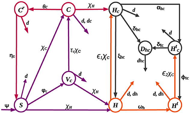
Figure 1. HIV and COVID-19 co-infection model flow diagram.

Given the aforementioned assumptions and descriptions, we hereby formulate the following systems of non-linear differential equations:

$\begin{array}{ll}\{\begin{array}{l}{S}^{\prime }=\psi -({\beta }_1+{\chi }_{{}_C}+{\chi }_{{}_H})S+{\eta }_c{C}^r\\ V_c^{\prime }={\phi }_{c}S-({\tau }_v{\chi }_{{}_C}+{\chi }_{{}_H}+d)V_c\\ C^{\prime }={\chi }_{{}_C}S+{\tau }_v{\chi }_{{}_C}{V}_c-({\beta }_2+{\chi }_{{}_H})C\\ {C^r}^{\prime }={\theta }_{c}C-{\beta }_3{C}^r\\ H^{\prime }=(S+V_c){\chi }_{{}_H}+{\xi }_{hc}{H}_c-({\beta }_4+{ϵ}_1{\chi }_{{}_C})H\\ {H^t}^{\prime }={\omega }_{h}H+{\varphi }_{tc}{H}_c^t-({\beta }_5+{ϵ}_2{\chi }_{{}_C})H^t\\ H_c^{\prime }={ϵ}_1{\chi }_{{}_C}H+{\chi }_{{}_H}C-{\beta }_6{H}_c\\ {H_c^t}^{\prime }={ϵ}_2{\chi }_{{}_C}{H}^t+{\alpha }_{hc}{H}_c-{\beta }_7{H}_c^t\\ D_{hc}^{\prime }={\delta }_{hc}{H}_c+{\delta }_{tc}{H}_c^t-{\beta }_8{D}_{hc}\end{array}& (1)\end{array}$

where β₁ = φ_c + d, β₂ = d_c + d + θ_c, β₃ = d + η_c, β₄ = ω_h + d + d_h, β₅ = d_h + d, β₆ = d + α_hc + ξ_hc + δ_hc, β₇ = d + ϕ_tc + δ_tc, and β₈ = d_hc + d.

The initial conditions of the equations of the model (1) are as follows:

$\begin{array}{ll}\{\begin{array}{l}S(0)=S_0,V_c(0)={V_c}_0,C(0)=C_0,C^r(0)=C_0^r,H(0)=H_0,\\ H^t(0)=H_0^t,H_c(0)={H_c}_0,\\ H_c^t(0)={H_c^t}_0,D_{hc}(0)={D_{hc}}_0.\end{array}& (2)\end{array}$

3 Model analysis

This section outlines the qualitative properties of Equation 1. This includes the existence and uniqueness of positive and bounded solutions and the stability of equilibria.

3.1 Invariant set, positivity, and boundedness of solutions

The positivity and boundedness of solutions are established in the following theorem.

Theorem 1. Assuming that all initial conditions in Equation 2 are positive, the solutions of the system (1) remain positive for all t > 0. Furthermore, the set

$\text{Υ}=\left\{(S,V_c,C,C^r,H,H^t,H_c,H_c^t,D_{hc})\in {ℝ}^9:0\le N\le \psi /d\right\}$

is a positively invariant region and serves as an attracting set for system (1).

Proof. It follows from the first equation of system (1) that, $\frac{dS}{dt}|{}_{S=0}=\psi +{\eta }_c{C}^r>0.$ We can see that S(t) remains positive ∀t > 0, which implies, the solution cannot exit Υ by crossing the boundary S = 0. Similarly, it is easy to show that $V_c,C,C^r,H,H^t,H_c,H_c^t,D_{hc}>0$, for all t > 0. Furthermore, N(t) satisfy $\frac{dN}{dt}\le \psi -dN$. Thus, we can deduce that 0 ≤ N ≤ ψ/d. Hence, all solutions in ${ℝ}_{+}^9$ are attracted to the region Υ. By Lemma 1 from [28], we can deduce that Υ is an invariant and positively defined set.

Theorem 1 confirms the epidemiological soundness of model (1), establishing the positivity and boundedness of all state variables. In other words, no solution path can extend beyond the boundaries of Υ, rendering it adequate to focus on the dynamics of system (1) within the confines of Υ. As the right-hand side of Equation 1 is locally Lipschitz, the existence of solutions follows from the Picard-Lindelöf Theorem [29]. Therefore, we establish the following theorem.

Theorem 2. Solutions to system (1) exist and are unique for all t ≥ 0.

From Theorem 1 and Theorem 2, we can deduce that model (1) is epidemiologically meaningful and mathematically well-posed.

3.2 HIV-only sub-model

Setting the state variables related to COVID-19 and co-infection equal to zero, $C=C^r=H_c=H_c^t=D_{hc}=0$, gives the following HIV-only sub-model:

$\begin{array}{ll}\{\begin{array}{l}{S}^{\prime }=\psi -({\beta }_1+{\chi }_{{}_H})S\\ V_c^{\prime }={\phi }_{c}S-({\chi }_{{}_H}+d)V_c\\ H^{\prime }=(S+V_c){\chi }_{{}_H}-{\beta }_{4}H\\ {H^t}^{\prime }={\omega }_{h}H-{\beta }_5{H}^t\end{array}& (3)\end{array}$

where ${\chi }_{{}_H}={\pi }_h\frac{H+H^t}{N}$.

To identify equilibrium points, HIV-free and endemic, we set the right-hand side of Equation 3 equal to 0. Thus, HIV-free equilibrium($E_h^0$), obtained when H = H^t = 0, is given by $E_h^0=(\frac{\psi }{{\beta }_1},\frac{{\phi }_c\psi }{d{\beta }_1},0,0)$.

The next-generation matrix result in [30] is employed to find the basic reproduction numbers of the sub- and co-infection models. Thus, the reproduction number($R_0^h$) of the HIV-only sub-model (3) is determined as

$\begin{array}{ll}{R}_0^h=\frac{{\pi }_h}{{\beta }_5}& (4)\end{array}$

Theorem 3. $E_h^0$, whenever $R_0^h<1$, is locally asymptotically stable.

Proof. The Jacobian of Equation 3 becomes

$\begin{array}{l}\left(\begin{array}{cccc}-{\beta }_1& 0& -\frac{d{\pi }_h}{{\beta }_1}& -\frac{d{\pi }_h}{{\beta }_1}\\ {\phi }_c& -d& -\frac{{\phi }_c{\pi }_h}{{\beta }_1}& -\frac{{\phi }_c{\pi }_h}{{\beta }_1}\\ 0& 0& {\pi }_h-{\beta }_4& {\pi }_h\\ 0& 0& {\omega }_h& -{\beta }_5\end{array}\right)\end{array}$

It is evident that −d, −β₁, and −β₆ are all negative. Two other eigenvalues are found in the matrix

$\begin{array}{l}\left(\begin{array}{cc}{\pi }_h-{\beta }_4& {\pi }_h\\ {\omega }_h& -{\beta }_5\end{array}\right)\end{array}$

Accordingly, the characteristic polynomial becomes $P(\lambda )={\lambda }^2+({\beta }_4+{\beta }_5-{\pi }_h)\lambda +{\beta }_4{\beta }_5(1-R_0^h).$ The local stability of $E_h^0$ is determined by the sign of the roots of P(λ) = 0. When $R_0^h<1$, the Routh-Hurwitz criterion leads us to the conclusion that all roots of P(λ) = 0 are negative, establishing the local asymptotic stability of $E_h^0$. Conversely, if $R_0^h>1$, the disease-free equilibrium becomes unstable due to the presence of a positive eigenvalue.

The epidemiological interpretation of the local stability of a disease-free equilibrium suggests that an epidemic is unlikely to occur, and there exists a potential for eliminating the disease from the population, especially when the flow of infectious individuals is relatively small. Specifically, Theorem 3 implies the feasibility of controlling HIV transmission by reducing $R_0^h$ below one.

If $R_0^h>1$, we obtain the endemic equilibrium point $E_h=(S^{*},V_c^{*},H^{*},{H^t}^{*})$, where

$\begin{array}{l}{S}^{*}=\frac{\psi }{{\beta }_1+{\beta }_5(R_0^H-1)},V^{*}=\\ \hspace{1em}\frac{{\phi }_c\psi }{\left[{\beta }_1+{\beta }_5(R_0^h-1)\right]\left[d+{\beta }_5(R_0^h-1)\right]},\\ {H^t}^{*}=\frac{{\omega }_h\psi (R_0^h-1)}{{\beta }_4\left[d+{\beta }_5(R_0^h-1)\right]}\text{ and }{H}^{*}=\frac{{\beta }_5\psi (R_0^h-1)}{{\beta }_4\left[d+{\beta }_5(R_0^h-1)\right]}.\end{array}$

Consequently, we can say that HIV persists in the population for $R_0^h>1$. However, for $R_0^H<1$, we can see that H^*,^Ht* < 0, which is biologically meaningless. Therefore, the theorem presented below has been established.

Theorem 4. Model (3), whenever $R_0^h>1$, has a unique endemic equilibrium.

3.3 COVID-19 only sub-model

Setting $H=H^t=H_c=H_c^t=D_{hc}=0$ yields the following sub-model of COVID-19:

$\begin{array}{ll}\{\begin{array}{l}{S}^{\prime }=\psi -({\beta }_1+{\chi }_{{}_C})S+{\eta }_c{C}^r\\ V_c^{\prime }={\phi }_{c}S-({\tau }_v{\chi }_{{}_C}+d)V_c\\ C^{\prime }={\chi }_{{}_C}S+{\tau }_v{\chi }_{{}_C}{V}_c-{\beta }_{2}C\\ {C^r}^{\prime }={\theta }_{c}C-{\beta }_3{C}^r\end{array}& (5)\end{array}$

where ${\chi }_{{}_C}={\pi }_c\frac{C}{N}$.

The COVID-19-free equilibrium($E_c^0$) is $E_c^0=(\frac{\psi }{{\beta }_1},\frac{{\phi }_c\psi }{d{\beta }_1},0,0)$, and the COVID-19 sub-model's reproduction number($R_0^c$) is determined as $R_0^c=\frac{(d+{\phi }_c{\tau }_v){\pi }_c}{{\beta }_1{\beta }_2}.$ In simpler terms, the epidemiological interpretation of the first and second terms of $R_0^c$ is that they represent the number of secondary infections that can be produced by one COVID-19-infected individual in susceptible and vaccinated class, respectively. Without vaccination, when φ_c, τ_v = 0, $R_0^c$ is given by $R_0^c={\hat{R}}_0^c=\frac{{\pi }_c}{{\beta }_2}.$ and $R_0^c$ can be expressed as $R_0^c=\frac{(d+{\phi }_c{\tau }_v){R_0^c}^{*}}{{\beta }_1}.$ This implies that the critical vaccination proportion that will lead to COVID-19 eradication is $\frac{d(1-{R_0^c}^{*})}{1-{\tau }_v{R_0^c}^{*}}$, which can be obtained by letting $R_0^c=1$ and solving for φ_c.

Theorem 5. $E_c^0$ is locally asymptotically stable, whenever $R_0^c<1$.

Proof. The Jacobian of system (5) at $E_0^c$ is

$\begin{array}{ll}\left(\begin{array}{cccc}-{\beta }_1& 0& -\frac{{\pi }_{c}d}{{\phi }_c+d}& {\eta }_c\\ {\phi }_c& -d& -\frac{{\pi }_c{\phi }_c{\tau }_v}{{\phi }_c+d}& 0\\ 0& 0& \frac{{\pi }_c({\phi }_c{\tau }_v+d)}{{\phi }_c+d}-{\beta }_2& 0\\ 0& 0& {\theta }_c& -{\beta }_3\end{array}\right).& (6)\end{array}$

We can see that, whenever $R_0^c<1$, the eigenvalues of matrix (6) are all negative. This means that when $R_0^c<1$, an outbreak cannot be caused by COVID-19-infected individuals and the disease can be eliminated.

The endemic equilibrium point $E_c=(S^{*},V_c^{*},C^{*},{C^r}^{*})$ is computed as follows:

$\begin{array}{ll}\begin{array}{c}{S}^{*}=\frac{{\beta }_2{\beta }_3\psi ({\tau }_v{\chi }_{{}_C}+d)}{{\tau }_v\left[{\beta }_2{\beta }_3-{\eta }_c{\theta }_c\right]{\chi }_{{}_C}^2+\left[({\tau }_v{\phi }_c+d)({\beta }_2{\beta }_3-{\eta }_c{\theta }_c)+{\tau }_v{\beta }_2{\beta }_{3}d\right]{\chi }_{{}_C}+{\beta }_1{\beta }_2{\beta }_{3}d}\\ V_c^{*}=\frac{{\phi }_c{\beta }_2{\beta }_3\psi }{{\tau }_v\left[{\beta }_2{\beta }_3-{\eta }_c{\theta }_c\right]{\chi }_{{}_C}^2+\left[({\tau }_v{\phi }_c+d)({\beta }_2{\beta }_3-{\eta }_c{\theta }_c)+{\tau }_v{\beta }_2{\beta }_{3}d\right]{\chi }_{{}_C}+{\beta }_1{\beta }_2{\beta }_{3}d}\\ C^{*}=\frac{{\beta }_3\psi {\chi }_{{}_C}({\tau }_v{\chi }_{{}_C}+{\phi }_c{\tau }_v+d)}{{\tau }_v\left[{\beta }_2{\beta }_3-{\eta }_c{\theta }_c\right]{\chi }_{{}_C}^2+\left[({\tau }_v{\phi }_c+d)({\beta }_2{\beta }_3-{\eta }_c{\theta }_c)+{\tau }_v{\beta }_2{\beta }_{3}d\right]{\chi }_{{}_C}+{\beta }_1{\beta }_2{\beta }_{3}d}\\ {C^r}^{*}=\frac{\psi {\theta }_c{\chi }_{{}_C}({\tau }_v{\chi }_{{}_C}+{\phi }_c{\tau }_v+d)}{{\tau }_v\left[{\beta }_2{\beta }_3-{\eta }_c{\theta }_c\right]{\chi }_{{}_C}^2+\left[({\tau }_v{\phi }_c+d)({\beta }_2{\beta }_3-{\eta }_c{\theta }_c)+{\tau }_v{\beta }_2{\beta }_{3}d\right]{\chi }_{{}_C}+{\beta }_1{\beta }_2{\beta }_{3}d}\end{array}& (7)\end{array}$

Substituting S^*, $V_c^{*}$, C^*, and ^Cr* of Equation 7 into ${\chi }_{{}_C}^{*}=\frac{{\pi }_c{C}^{*}}{S^{*}+V_c^{*}+C^{*}+{C^r}^{*}}$ yields ${\chi }_{{}_C}^{*}(q_2{\chi }_{{}_C}^{{*}^2}+q_1{\chi }_{{}_C}^{*}+q_0)=0$, where $q_0={\beta }_1{\beta }_2{\beta }_3(1-R_0^c)$, q₁ = τ_vβ₂β₃+(d+τ_vφ_c)(β₃+θ_c) − π_cτ_vβ₃, and q₂ = τ_v(β₃+θ_c). For ${\chi }_{{}_C}^{*}=0$, we obtain the disease-free equilibrium $E_0^c$. Thus, the endemic equilibrium satisfies the following equation:

$\begin{array}{ll}{q}_2{\chi }_{{}_C}^{{*}^2}+q_1{\chi }_{{}_C}^{*}+q_0=0.& (8)\end{array}$

The solution of ${\chi }_{{}_C}^{*}$ is given by ${\chi }_{{}_C}^{*}=\frac{-q_1\pm \sqrt{q_1^2-4q_0{q}_2}}{2q_2}.$ To assess the potential for an endemic equilibrium in Equation 5, we explore two distinct scenarios, emphasizing positive real solutions while excluding the possibility of negative and complex solutions in Equation 8. Consequently, we observe that Equation 8:

1. possesses a unique positive solution if $R_0^c>1$ and

2. exhibits two positive solutions if $R_0^c<1$ and q₁ < 0.

The second condition indicates the backward bifurcation phenomenon, the co-existence of a stable endemic and COVID-19-free equilibria, even if $R_0^c<1$. For τ_v = 0 and/or φ_c = 0, we obtain q₁ > 0, implying that the imperfect vaccine can cause the backward bifurcation.

3.4 The influence of HIV on the endemic chapter of COVID-19

Even though the World Health Organization has classified COVID-19 as a persistent health challenge, no longer deeming it a public health emergency of international concern [31], it continues to pose a significant threat to global health. This section will focus on investigating the contribution of HIV to the transmission of COVID-19. Hence, we write d in Equation 4 in terms of $R_0^h$ to express $R_0^c$ in terms of $R_0^h$. That is, $d=\frac{{\pi }_h-R_0^h{d}_h}{R_0^h}.$ Upon replacing this d value in $R_0^c$, we obtain $R_0^c=\frac{R_0^h{\pi }_c({\pi }_h+R_0^h({\phi }_c{\tau }_v-d_h))}{({\pi }_h+R_0^h({\phi }_c-d_h))(R_0^h(d_c-d_h+{\theta }_c)+{\pi }_h)},$ which implies,

$\frac{\partial R_0^c}{\partial R_0^h}=\frac{{({\pi }_h-R_0^h(d_h+{\phi }_c{\tau }_v))}^2+(1-{\tau }_v){\phi }_c{R_0^h}^2({\phi }_c{\tau }_v-{\theta }_c-d_c)}{{({\pi }_h+R_0^h({\phi }_c-d_h))}^2{(R_0^h(d_c-d_h+{\theta }_c)+{\pi }_h)}^2}.$

In the community, when $\frac{\partial R_0^c}{\partial R_0^h}>0$ (that is when $\frac{{({\pi }_h-R_0^h(d_h+{\phi }_c{\tau }_v))}^2+(1-{\tau }_v){\tau }_v{{\phi }_c}^2{R_0^h}^2}{{\phi }_c(1-{\tau }_v)({\theta }_c+d_c){R_0^h}^2}>1$), there is a corresponding rise in COVID cases as the number of HIV cases increases. The positive correlation between the two implies that targeted interventions and health campaigns within communities where both HIV and COVID-19 are prevalent are necessary to combat the transmission of these infections.

3.5 Co-infection model analysis

The disease-free equilibrium, $E^0$, is given by $E^0=(\frac{\psi }{{\beta }_1},\frac{{\phi }_c\psi }{{\beta }_{1}d},0,0,0,0,0,0,0,0,0).$ The reproduction number ($R_0$) for the COVID-19 and HIV co-infection model is obtained as $R_0=max\left\{R_0^c,R_0^h\right\}.$ Furthermore, the subsequent theorem is established by employing Theorem 2 introduced in [30].

Theorem 6. $E^0$ is unstable if $R_0>1$ and locally asymptotically stable if $R_0<1$.

To assess the global stability of $E^0$, we employ the method described in [32]. By adopting the notation from [32] and rephrasing system (1) as Equation (3.1) of [32], we obtain

$\begin{array}{l}\widehat{G}(\text{X},\text{I})=\left(\begin{array}{c}{\pi }_c(C+H_c+H_c^t)(\frac{S(0)}{N(0)}-\frac{S}{N}+{\tau }_v(\frac{V_c(0)}{N(0)}-\frac{V_c}{N}))+{\chi }_{{}_H}C\\ {\pi }_h(H+H^t+H_c+H_c^t)(1-\frac{S+V_c+C^r}{N})+{\chi }_{{}_C}H\\ {\chi }_{{}_C}{H}^t\\ -{\chi }_{{}_C}H-{\chi }_{{}_H}C\\ -{\chi }_{{}_C}{H}^t\\ 0\end{array}\right)\end{array}$

where $\text{I}=(C,H,H^t,H_c,H_c^t,D_{hc})$ and $\text{X}=(S,V_c,C^r)$ denote infected and uninfected population, respectively.

The fourth and fifth rows of Ĝ(X, I) are less than zero. So, the assumption H2 in [32] is not satisfied. This suggests that $E^0$ might not be globally asymptotically stable. That is, system (1) exhibits backward bifurcation, as proved by the following theorem.

Theorem 7. System (1) undergoes a backward bifurcation at $R_0=1$ when

$\begin{array}{l}{\tau }_v(1-{\tau }_v){\phi }_c{\beta }_2-{({\tau }_v{\phi }_c+d)}^2(1+\frac{{\theta }_c}{{\beta }_3})>0.\end{array}$

Proof. The central manifold approach introduced in [33] is used to show existence of backward bifurcation in system (1). Thus, the following change of variables is introduced: ${\tilde{z}}_1=S,{\tilde{z}}_2=V_c,{\tilde{z}}_3=C,{\tilde{z}}_4=C^r,{\tilde{z}}_5=H,{\tilde{z}}_6=H^t,{\tilde{z}}_7=H_c,{\tilde{z}}_8=H_c^t,\mathrm{\text{and}}{\tilde{z}}_9=D_{hc}.$So that, $N=\sum _{j=1}^9{\tilde{z}}_j,{\chi }_{{}_C}={\pi }_h\frac{{\tilde{z}}_3+{\tilde{z}}_7+{\tilde{z}}_8}{N-{\tilde{z}}_9},\mathrm{\text{and}}{\chi }_{{}_H}={\pi }_h\frac{{\tilde{z}}_5+{\tilde{z}}_6+{\tilde{z}}_7+{\tilde{z}}_8}{N-{\tilde{z}}_9}.$

Moreover,

$\begin{array}{ll}{\tilde{z}}^{\prime }=\text{p}={(p_1,p_2,p_3,p_4,p_5,p_6,p_7,p_8,p_9)}^T& (9)\end{array}$

is used to express system (1) with $\tilde{z}={({\tilde{z}}_1,{\tilde{z}}_2,{\tilde{z}}_3,{\tilde{z}}_4,{\tilde{z}}_5,{\tilde{z}}_6,{\tilde{z}}_7,{\tilde{z}}_8,{\tilde{z}}_9)}^T$.

Suppose $R_0=max\left\{R_0^c,R_0^h\right\}=R_0^c$. After selecting π_c as the bifurcation parameter and setting $R_0^c=1$, we get ${\pi }_c={\pi }_c^{*}=\frac{{\beta }_1{\beta }_2}{{\tau }_v{\phi }_c+d}.$ At $E^0$, the Jacobian of the system (9) for ${\pi }_c={\pi }_c^{*}$ has a simple zero eigenvalue, but the real part of all other eigenvalues are negative. Consequently, we used the notion in [33] and performed the following calculations.

For zero eigenvalue, we have the right eigenvector ${(w_1,w_2,w_3,w_4,w_5,w_6,w_7,w_8,w_9)}^T$ and left eigenvector (v₁, v₂, v₃, v₄, v₅, v₆, v₇, v₈, v₉), where

$\begin{array}{l}{w}_1=\frac{w_3}{{\beta }_1}(\frac{{\theta }_c{\eta }_c}{{\beta }_3}-\frac{{\pi }_c^{*}d}{{\beta }_1}),w_2=\frac{{\phi }_c}{d}(w_1-\frac{{\tau }_v{\pi }_c^{*}{w}_3}{{\beta }_1}),\\ w_3>0,w_4=\frac{w_3{\theta }_c}{{\beta }_3},v_3>0,\\ v_7=\frac{{\beta }_2({\alpha }_{hc}+{\beta }_7)v_3}{{\beta }_6{\beta }_7},v_8=\frac{{\beta }_2{v}_3}{{\beta }_7},\text{ and }{w}_5,w_6,w_7,w_8,w_9,v_1,v_2,v_4,\\ v_5,v_6,v_9=0.\end{array}$

The values of a and b are calculated as follows:

$\begin{array}{l}a={\displaystyle \sum _{k,i,j=1}^9}{v}_k{w}_i{w}_j\frac{{\partial }^2{\tilde{p}}_k}{\partial {\tilde{z}}_i\partial {\tilde{z}}_j}(E^0,{\pi }_c^{*})\\ \hspace{1em}={\displaystyle \sum _{i,j=1}^9}[v_3{w}_i{w}_j\frac{{\partial }^2{\tilde{p}}_3}{\partial {\tilde{z}}_i\partial {\tilde{z}}_j}(E^0,{\pi }_c^{*})+v_7{w}_i{w}_j\frac{{\partial }^2{\tilde{p}}_7}{\partial {\tilde{z}}_i\partial {\tilde{z}}_j}(E^0,{\pi }_c^{*})+\\ \hspace{1em}\hspace{1em}{v}_8{w}_i{w}_j\frac{{\partial }^2{\tilde{p}}_8}{\partial {\tilde{z}}_i\partial {\tilde{z}}_j}(E^0,{\pi }_c^{*})]\\ \hspace{1em}=\frac{2d{\beta }_2{v}_3{w}_3^2}{\psi {({\tau }_v{\phi }_c+d)}^2}({\tau }_v(1-{\tau }_v){\phi }_c{\beta }_2-{({\tau }_v{\phi }_c+d)}^2(1+\frac{{\theta }_c}{{\beta }_3}))\end{array}$

and

$\begin{array}{l}b={\displaystyle \sum _{k,j=1}^9}{v}_k{w}_j\frac{{\partial }^2{\tilde{p}}_k}{\partial {\tilde{z}}_j\partial {\pi }_c}(E^0,{\pi }_c^{*})\\ \hspace{1em}={\displaystyle \sum _{i,j=1}^9}[v_3{w}_i{w}_j\frac{{\partial }^2{\tilde{p}}_3}{\partial {\tilde{z}}_i\partial {\pi }_c}(E^0,{\pi }_c^{*})+v_7{w}_i{w}_j\frac{{\partial }^2{\tilde{p}}_7}{\partial {\tilde{z}}_i\partial {\pi }_c}(E^0,{\pi }_c^{*})+\\ \hspace{1em}\hspace{1em}{v}_8{w}_i{w}_j\frac{{\partial }^2{\tilde{p}}_8}{\partial {\tilde{z}}_i\partial {\pi }_c}(E^0,{\pi }_c^{*})]\\ \hspace{1em}=\frac{v_3{w}_3({\tau }_v{\phi }_c+d)}{{\beta }_1}>0.\end{array}$

The coefficient b remains positive. Therefore, at $R_0=1$, backward bifurcation is exhibited, when a > 0. It is obvious that a < 0 when the vaccination is perfect(τ_v = 0). Hence, as per Theorem 4.1 in [33], system (1) will experience a trans-critical bifurcation at $R_0$. This indicates that the backward bifurcation characteristic of the co-infection model (1) emerges from an imperfect vaccine, a common cause for backward bifurcation [34].

4 Model extension to include optimal control

This section introduces four Lebesgue measurable control functions of time to model (1). The following is a description of these control functions:

u₁(t): steps made to promote and supply the COVID-19 vaccination,

u₂(t): initiatives aimed at preventing the spread of HIV,

u₃(t): measures taken to reduce the COVID-19 burden through treatment and

u₄(t): the use of antiretroviral therapy (ART) for HIV patients.

To make things simple, we will define $x=(S,V_c,C,C^r,H,H^t,H_c,H_c^t)$ and u = (u₁, u₂, u₃, u₄).

Upon including u₁, u₂, u₃, and u₄ into Equation 1, we derive the optimal control model as follows:

$\begin{array}{l}\{\begin{array}{l}{S}^{\prime }=\psi -({\beta }_1+u_1+{\chi }_{{}_C}+(1-u_2){\chi }_{{}_H})S+{\eta }_c{C}^r\\ V_c^{\prime }=({\phi }_c+u_1)S-({\tau }_v{\chi }_{{}_C}+(1-u_2){\chi }_{{}_H}+d)V_c\\ C^{\prime }={\chi }_{{}_C}S+{\tau }_v{\chi }_{{}_C}{V}_c-({\beta }_2+u_3+(1-u_2){\chi }_{{}_H})C\\ {C^r}^{\prime }=(u_3+{\theta }_c)C-{\beta }_3{C}^r\\ \end{array}\end{array}$

$\begin{array}{ll}\{\begin{array}{l}{H}^{\prime }=(1-u_2)(S+V_c){\chi }_{{}_H}+(u_3+{\xi }_{hc})H_c-({\beta }_4+u_4+{ϵ}_1{\chi }_{{}_C})H\\ {H^t}^{\prime }=(u_4+{\omega }_h)H+(u_3+{\varphi }_{tc})H_c^t-({\beta }_5+{ϵ}_2{\chi }_{{}_C})H^t\\ H_c^{\prime }={ϵ}_1{\chi }_{{}_C}H+(1-u_2){\chi }_{{}_H}C-({\beta }_6+u_3+u_4)H_c\\ {H_c^t}^{\prime }={ϵ}_2{\chi }_{{}_C}{H}^t+(u_4+{\alpha }_{hc})H_c-({\beta }_7+u_3)H_c^t\\ D_{hc}^{\prime }={\delta }_{hc}{H}_c+{\delta }_{tc}{H}_c^t-{\beta }_8{D}_{hc}\end{array}& (10)\end{array}$

subject to Equation 2.

The controls u₁ and u₃ in Equation 10 were added to the existing parameters to increase the vaccination rates as well as the rate of recovery of COVID-19, respectively. Moreover, adding u₄ represents an increase in HIV treatment efforts. Furthermore, using u₂ as a multiplicative effect represents a proportional reduction in HIV transmission rates. The aim of introducing u₁, u₂, u₃, and u₄ in Equation 1 is to identify the most cost-effective intervention strategy to reduce HIV and COVID-19 co-infection cases. To accomplish this, the following objective function is established.

$\begin{array}{ll}J(u)={\displaystyle {\int }_0^{t_f}}F(t,x,u)dt& (11)\end{array}$

where $F(t,x,u)=a_{1}C+a_{2}H+a_3{H}^t+a_4{H}_c+a_5{H}_c^t+a_6{D}_{hc}+\frac{1}{2}\sum _{j=1}^4{B}_j{u}_j^2$ and t_f is the final time.

The state variables, along with the balancing weight parameters a₁, a₂, a₃, a₄, a₅, and a₆ in F, are employed to minimize the number of co-infected individuals over a specific duration. The non-linear expression $B_i{u}_i^2$, consistent with previous studies [35, 36], represents the expenses associated with treatment and prevention, reflecting the inherently non-linear nature of costs. Thus, our goal is to determine the optimal control $u^{*}=(u_1^{*},u_2^{*},u_3^{*},u_4^{*})$ so that, given system (10) with initial conditions (2),

$\begin{array}{ll}J(u_1^{*},u_2^{*},u_3^{*},u_4^{*})={\displaystyle \underset{u\in U}{min}}J(u)& (12)\end{array}$

where $U=\left\{u|0\le u_j(t)\le 1,j=1,2,3,4,\mathrm{\text{for}}0\le t\le t_f\right\}$ is the set of admissible control functions.

Theorem 4.1 and Corollary 4.1 from [37] can be used to show the existence of solutions to Equation 12. Following the existence of the solutions, we employ Pontryagin's minimum principle to characterize the optimal controls.

4.1 Necessary conditions

To use Pontryagin's minimum principle, first, we transform the optimal control problem (12) into a point-wise Hamiltonian, G, minimization problem:

$\begin{array}{l}G=F(t,x,u)+{\displaystyle \sum _{j=1}^9}{l}_j{\tilde{f}}_j(t,x,u)\end{array}$

where l_j, also known as the adjoint variables, are piecewise differentiable functions that need to be found, and ${\tilde{f}}_j$ represents the right-hand side of the ith equation of system (10).

Theorem 8. Suppose ${\widehat{x}}_1=S,{\widehat{x}}_2=V_c,{\widehat{x}}_3=C,{\widehat{x}}_4=C^r,{\widehat{x}}_5=H,{\widehat{x}}_6=H^t,{\widehat{x}}_7=H_c,{\widehat{x}}_8=H_c^t$ and ${\widehat{x}}_9=D_{hc}$ be optimal state solutions and u^* be the corresponding control set for the optimal control problem (10) and (11). Then, the adjoint variables satisfy

$\begin{array}{ll}\frac{d{l}_i}{dt}=-\frac{\partial G}{\partial {\widehat{x}}_j}& (13)\end{array}$

with transversality conditions l_j(t_f) = 0, for j = 1, 2, 3, ..., 9. Furthermore, the control set u^* is characterized by

$\begin{array}{l}{u}_1^{*}=max\left\{0,min\left\{1,\frac{(l_1-l_2)S}{B_1}\right\}\right\}\\ u_2^{*}=max\left\{0,min\left\{1,\frac{{\chi }_H((l_5-l_1)S+(l_5-l_2)V_c)+C(l_7-l_3)}{B_2}\right\}\right\}\\ u_3^{*}=max\left\{0,min\left\{1,\frac{(l_7-l_5)H_c+C(l_3-l_4)+(l_8-l_6){\displaystyle \underset{c}{\overset{t}{H}}}}{B_3}\right\}\right\}\\ u_4^{*}=min\left\{0,min\left\{1,\frac{(l_7-l_8)H_c+H(l_5-l_6)}{B_4}\right\}\right\}& (14)\end{array}$

Proof. By differentiating the Hamiltonian with respect to the state variables, we derive the following differential equation governing the adjoint variables.

$\begin{array}{l}\frac{d{l}_1}{dt}=(({\chi }_{{}_C}+Q_1)L_1+{\beta }_1+u_1)l_1-\left(\frac{({\tau }_v{\chi }_{{}_C}+Q_1)V_c}{N}+{\phi }_c+u_1\right)l_2-\\ \hspace{1em}\hspace{1em}\left(\frac{Q_{1}C}{N}+(1-\frac{Q_3}{N}){\chi }_{{}_C}\right)l_3\\ \hspace{1em}\hspace{1em}-\left(\frac{{ϵ}_1{\chi }_{{}_C}H}{N}+Q_1(1-\frac{Q_2}{N})\right)l_5-\frac{{ϵ}_2{\chi }_{{}_C}{H}^t{l}_6}{N}+\frac{(Q_{1}C+{ϵ}_1{\chi }_{{}_C}H)l_7}{N}+\\ \hspace{1em}\hspace{1em}\frac{l_8{ϵ}_2{\chi }_{{}_C}{H}^t}{N}\\ \frac{d{l}_2}{dt}=-\frac{l_1({\chi }_{{}_C}+Q_1)S}{N}+l_2(L_2({\tau }_v{\chi }_{{}_C}+Q_1)+d)-l_3\\ \hspace{1em}\hspace{1em}\left({\chi }_{{}_C}({\tau }_v-\frac{Q_3}{N})+\frac{Q_{1}C}{N}\right)\\ \hspace{1em}\hspace{1em}-l_5\left(\frac{{ϵ}_1{\chi }_{{}_C}H}{N}+Q_1(1-\frac{Q_2}{N})\right)-\frac{l_6{ϵ}_2{\chi }_{{}_C}{H}^t}{N}+l_7\left(\frac{Q_{1}C}{N}+\frac{{ϵ}_1{\chi }_{{}_C}H}{N}\right)+\\ \hspace{1em}\hspace{1em}\frac{l_8{ϵ}_2{\chi }_{{}_C}{H}^t}{N}\\ \frac{d{l}_3}{dt}=l_{1}S\left(Q_4-\frac{Q_1}{N}\right)+l_2{V}_c\left({\tau }_v{Q}_4-\frac{Q_1}{N}\right)+l_3(Q_1{L}_3-Q_3{Q}_4+{\beta }_2+u_3)-\\ \hspace{1em}\hspace{1em}(u_3+{\theta }_c)l_4\\ \hspace{1em}\hspace{1em}+l_5\left(\frac{Q_1{Q}_2}{N}+{ϵ}_1{Q}_{4}H\right)+{ϵ}_2{Q}_4{l}_6{H}^t-l_7(Q_1{L}_3+{ϵ}_1{Q}_{4}H)-\\ \hspace{1em}\hspace{1em}{ϵ}_2{Q}_4{l}_8{H}^t-a_1\\ \frac{d{l}_4}{dt}=-l_1\left(\frac{({\chi }_{{}_C}+Q_1)S}{N}+{\eta }_c\right)-\frac{l_2{V}_c(Q_1+{\tau }_v{\chi }_{{}_C})}{N}-l_3\\ \hspace{1em}\hspace{1em}\left(\frac{Q_{1}C}{N}-\frac{{\chi }_{{}_C}{Q}_3}{N}\right)+{\beta }_3{l}_4\\ \hspace{1em}\hspace{1em}-l_5\left(\frac{{ϵ}_1{\chi }_{{}_C}H}{N}-\frac{Q_1{Q}_2}{N}\right)-\frac{l_6{ϵ}_2{\chi }_{{}_C}{H}^t}{N}+l_7\left(\frac{Q_{1}C}{N}+\frac{{ϵ}_1{\chi }_{{}_C}H}{N}\right)+\\ \hspace{1em}\hspace{1em}\frac{l_8{ϵ}_2{\chi }_{{}_C}{H}^t}{N}\\ \frac{d{l}_5}{dt}=l_{1}S\left(Q_5-\frac{{\chi }_{{}_C}}{N}\right)+l_2{V}_c\left(Q_5-\frac{{\tau }_v{\chi }_{{}_C}}{N}\right)+l_3\left(\frac{{\chi }_{{}_C}{Q}_3}{N}+Q_{5}C\right)\\ \hspace{1em}\hspace{1em}+l_5({ϵ}_1{\chi }_{{}_C}{L}_4-Q_2{Q}_5+{\beta }_4+u_4)-l_6\left(\frac{{ϵ}_2{\chi }_{{}_C}{H}^t}{N}+{\omega }_h+u_4\right)-l_7\\ \hspace{1em}\hspace{1em}\hspace{1em}({ϵ}_1{\chi }_{{}_C}{L}_4+Q_{5}C)+\frac{{ϵ}_2{\chi }_{{}_C}{l}_8{H}^t}{N}-a_2\\ \frac{d{l}_6}{dt}=l_{1}S\left(Q_5-\frac{{\chi }_{{}_C}}{N}\right)+l_2{V}_c\left(Q_5-\frac{{\tau }_v{\chi }_{{}_C}}{N}\right)+l_3\left(\frac{{\chi }_{{}_C}{Q}_3}{N}+Q_{5}C\right)-l_5\\ \hspace{1em}\hspace{1em}\left(\frac{{ϵ}_1{\chi }_{{}_C}H}{N}+Q_2{Q}_5\right)+l_6({ϵ}_2{\chi }_{{}_C}{L}_5+{\beta }_5)-l_7\left(Q_{5}C-\frac{{\chi }_{{}_C}H}{N}\right)-l_8{ϵ}_2{\chi }_{{}_C}{L}_5-a_3\\ \frac{d{l}_7}{dt}=(Q_4+Q_5)l_{1}S+l_2{V}_c({\tau }_v{Q}_4+Q_5)-l_3(Q_3{Q}_4-Q_{5}C)-l_5\\ \hspace{1em}\hspace{1em}\hspace{1em}(-{ϵ}_1{Q}_{4}H+Q_2{Q}_5+u_3+{\xi }_{hc})\\ \hspace{1em}\hspace{1em}+{ϵ}_2{Q}_4{l}_6{H}^t-l_7(Q_{5}C+{ϵ}_1{Q}_{4}H-{\beta }_6-u_3-u_4)-l_8({ϵ}_2{Q}_4{H}^t+u_4+{\alpha }_{hc})-l_9\\ \hspace{1em}\hspace{1em}\hspace{1em}{\delta }_{hc}-a_4\\ \frac{d{l}_8}{dt}=(Q_4+Q_5)l_{1}S+l_2{V}_c({\tau }_v{Q}_4+Q_5)-l_3(Q_3{Q}_4-C{Q}_5)+l_5\\ \hspace{1em}\hspace{1em}\hspace{1em}\left({ϵ}_1{Q}_{4}H-Q_2{Q}_5\right)\\ \hspace{1em}\hspace{1em}-l_6(-{ϵ}_2{Q}_4{H}^t+u_3+{\varphi }_{tc})-l_7(Q_{5}C+{ϵ}_1{Q}_{4}H)-l_8({ϵ}_2{Q}_4{H}^t-{\beta }_7-u_3)-l_9\\ \hspace{1em}\hspace{1em}\hspace{1em}{\delta }_{tc}-a_5\\ \frac{d{l}_9}{dt}={\beta }_8{l}_9-a_6\end{array}$

where $Q_1=(1-u_2){\chi }_{{}_H},Q_2=S+V_c,Q_3=S+{\tau }_v{V}_c,Q_4=\frac{{\pi }_c-Q_1}{N},Q_5=\frac{(1-u_2){\pi }_h-Q_2}{N}$, $L_1=(1-\frac{S}{N}),L_2=(1-\frac{V_c}{N}),L_3=(1-\frac{C}{N}),L_4=(1-\frac{H}{N})$, and $L_5=(1-\frac{H^t}{N})$.

The characterization in Equation 14 is obtained by solving $u_j^{*}$ from $\frac{\partial G}{\partial u_j}=0$, where j = 1, 2, 3, ..., 9, and applying standard control arguments involving bounds on the controls.

5 Numerical simulations

This section presents numerical simulations to validate the qualitative analysis results of system (1) and illustrate the contribution of optimal control strategies on cases of COVID-19 and HIV co-infection. For this study, the total population and life expectancy of Ethiopia in 2021 have been taken into account. The estimated total population were N = 120, 283, 026 with a life expectancy of 65 years [38]. Consequently, $d=\frac{1}{(65\times 365)}$ per day and ψ = d × N = 5070 people per day. We employed parameter values from existing research, and where data were unavailable, we estimated certain parameters within acceptable ranges. Table 1 presents the parameter values used in the numerical simulations. For the numerical simulations, the following initial conditions were applied: S(0) = 120269406, V_c(0) = 8000, C(0) = 800, C^r(0) = 1200, H(0) = 1500, H^t(0) = 1800, H_c(0) = 150, $H_c^t(0)=120$, and D_hc(0) = 50.

Table 1

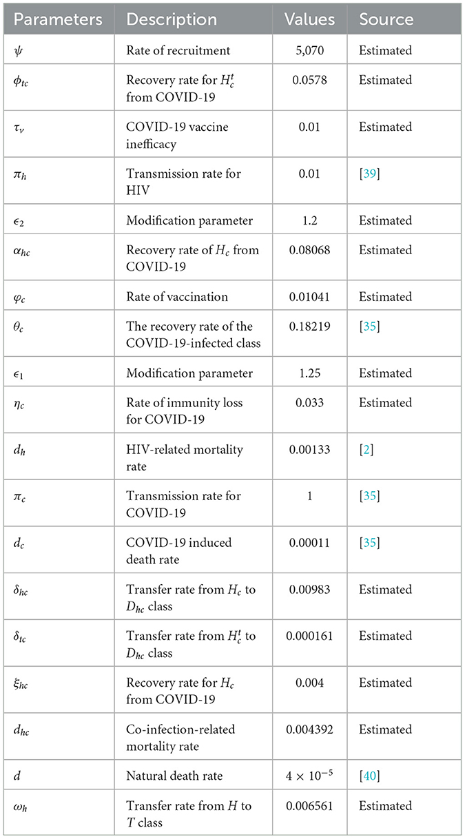
Table 1. Description of the parameters in Equation 1.

5.1 Simulations of the co-infection model

Figure 2B illustrates that even when $R_0^c$ is < 1, the state variables tend to converge toward positive values. This suggests that the COVID-19 sub-model exhibits a backward bifurcation phenomenon. Figure 2A indicates that the backward bifurcation occurs at $R_0^c=1$. For $R_0^c<1$, two endemic equilibria (stable and unstable) coexist with a stable disease-free equilibrium in the vicinity of $R_0^c=1$. The occurrence of a backward bifurcation is epidemiologically significant as it demonstrates that the condition of $R_0^c<1$ is necessary but not sufficient for disease control. This implies that eradicating COVID-19 can be challenging when a backward bifurcation phenomenon is present in the dynamics of disease transmission.

Figure 2

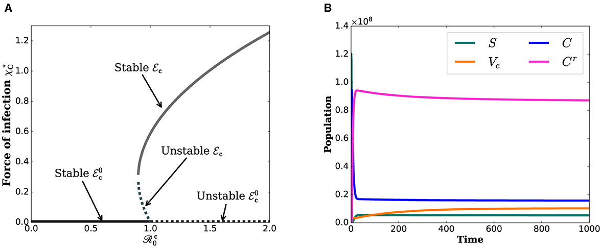
Figure 2. Simulations that show the backward bifurcation diagram and the existence of endemic equilibrium when $R_0^c=0.35$. (A) Bifurcation diagram. (B) State variables.

5.2 Simulations of the optimal control model

The optimal control problem (1) is analyzed iteratively using the Runge–Kutta forward-backward sweep numerical approximation method described in [41]. In line with this approach, first, a fourth-order Runge–Kutta method is employed to solve the state variable solutions forward in time with an initial guess for the control variables. Then, the solutions of the state variables are used to solve Equation 13 backward in time. Once the state and adjoint solutions are solved, the control is updated with these new values. These procedures are repeated until the solutions converge. In performing numerical simulation associated with the optimal control problem, the following set of values of costs are considered: B₁ = 30, B₂ = 20, B₃ = 50, and B₄ = 150. The weighted coefficients are further assumed to be a₁ = 100, a₂ = 100, a₃ = 50, a₄ = 120 , a₅ = 80, and a₆ = 150. The intention of setting a high weight coefficient value for D_hc is to minimize the loss of lives from HIV and COVID-19 infections. To examine the outcome of control strategies, we consider four different scenarios:

Scenario 1: use of single control strategy,

Scenario 2: implementing a combination of two control strategies,

Scenario 3: implementing a combination of three control strategies and

Scenario 4: implementing a combination of all control strategies.

Numerical results for all four scenarios are presented for the final time period of t_f = 120. In the following section, we will take a closer look at each scenario.

5.2.1 Scenario 1: use of single control strategy

Here, the following strategies are taken into account:

Strategy A: Vaccination only (u₁ ≠ 0)

Strategy B: Prevention for HIV only (u₂ ≠ 0)

Strategy C: Treatment for COVID-19 only (u₃ ≠ 0)

Strategy D: Treatment for HIV only (u₄ ≠ 0)

The effectiveness of the control strategies and their impact profiles are depicted in Figure 3. In Figure 3A, it is evident that COVID-19 and HIV treatment options significantly reduce the population in the H_c compartment compared to other strategies. The highest peak value in Figure 3B is attributed to an increase in HIV treatment efforts. However, this figure reveals the inverse outcome of COVID-19 treatment on the population in $H_c^t$. Figures 3C, H demonstrate that the treatment of COVID-19 is more crucial than other options in reducing the risk of mortality from co-infection. The calculations leading to Figures 3H, I are provided in Section 6.1. Overall, these figures illustrate that, in terms of consistently reducing the number of deaths, COVID-19 appears to contribute more effectively. In summary, the COVID-19 treatment approach seems to play a more significant role in consistently lowering the number of deaths.

Figure 3

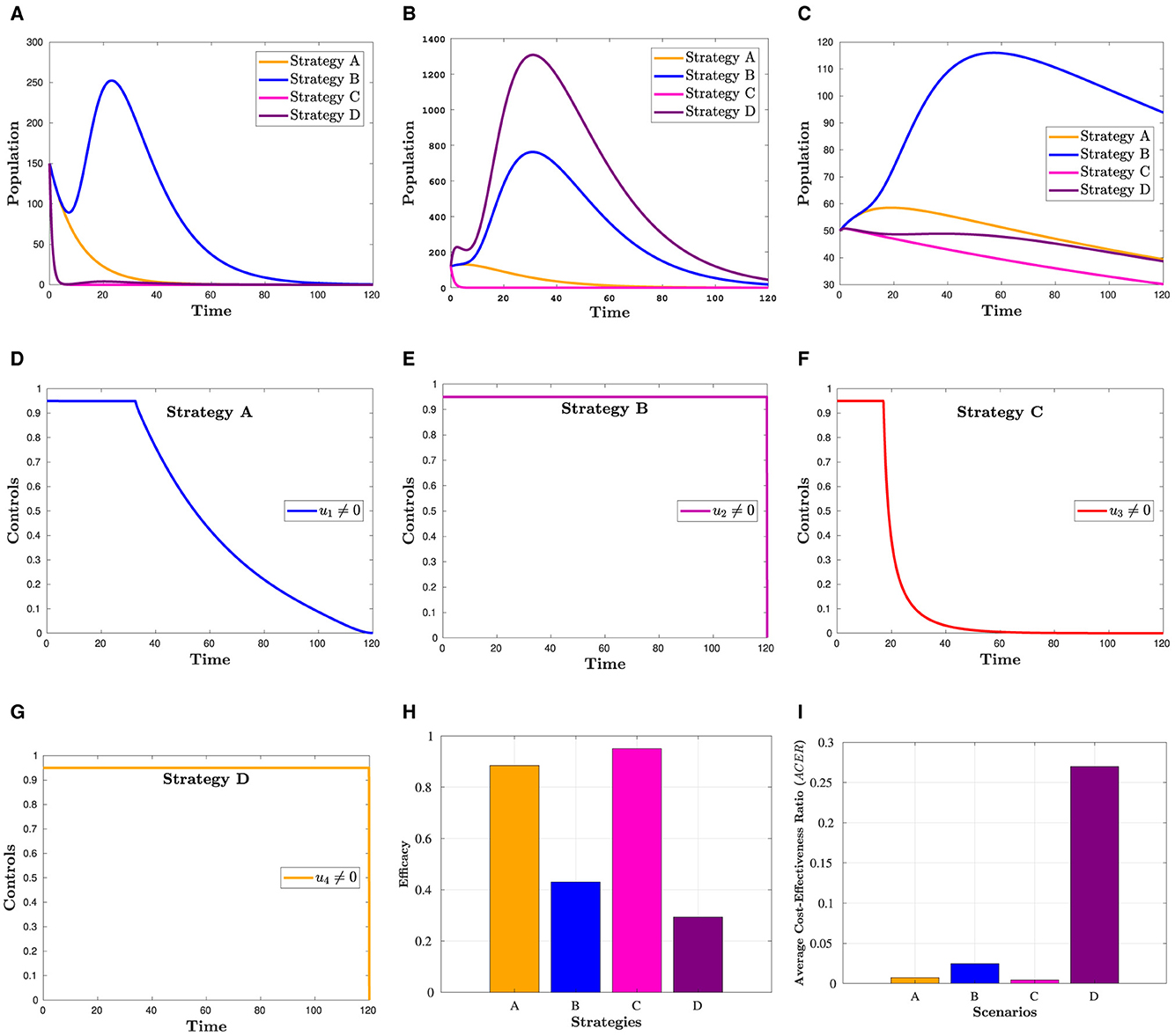
Figure 3. Simulation showing how scenario 1's strategies affect the outcome. (A) H_c population. (B) $H_c^t$ population. (C) D_hc population. (D) Control profile(u₁). (E) Control profile(u₂). (F) Control profile(u₃). (G) Control profile(u₄). (H) Efficacy of strategies in scenario 1. (I) Cost-effectiveness of strategies in scenario 1.

5.2.2 Scenario 2: use of combinations of two controls

This section examines the following combinations of two strategies.

Strategy E: COVID-19 vaccination and HIV prevention (u₁, u₂ ≠ 0)

Strategy F: Vaccination and treatment for COVID-19 (u₁, u₃ ≠ 0)

Strategy G: COVID-19 vaccination and treatment for HIV (u₁, u₄ ≠ 0)

Strategy H: Treatment for COVID-19 and prevention for HIV (u₂, u₃ ≠ 0)

Strategy I: Prevention and treatment for HIV (u₂, u₄ ≠ 0)

Strategy J: Treatment for COVID-19 and HIV (u₃, u₄ ≠ 0)

Figure 4 presents the simulation results for a combination of two control strategies. The figure indicates that the combinations of u₁ and u₃, u₂ and u₃, and u₃ and u₄ have resulted in the lowest number of co-infection cases and the lowest risk of mortality. This observation is reinforced by Figure 4J, which provides a detailed illustration of the effectiveness of each of the six measures, as discussed further in Section 6.2. Moreover, if these measures are to be implemented, u₂ and u₄ should remain at their maximum level until the intervention is over, as depicted in Figures 4D–I. In contrast, the control efforts u₁ and u₃ can gradually decrease from their maximum after a certain number of days.

Figure 4

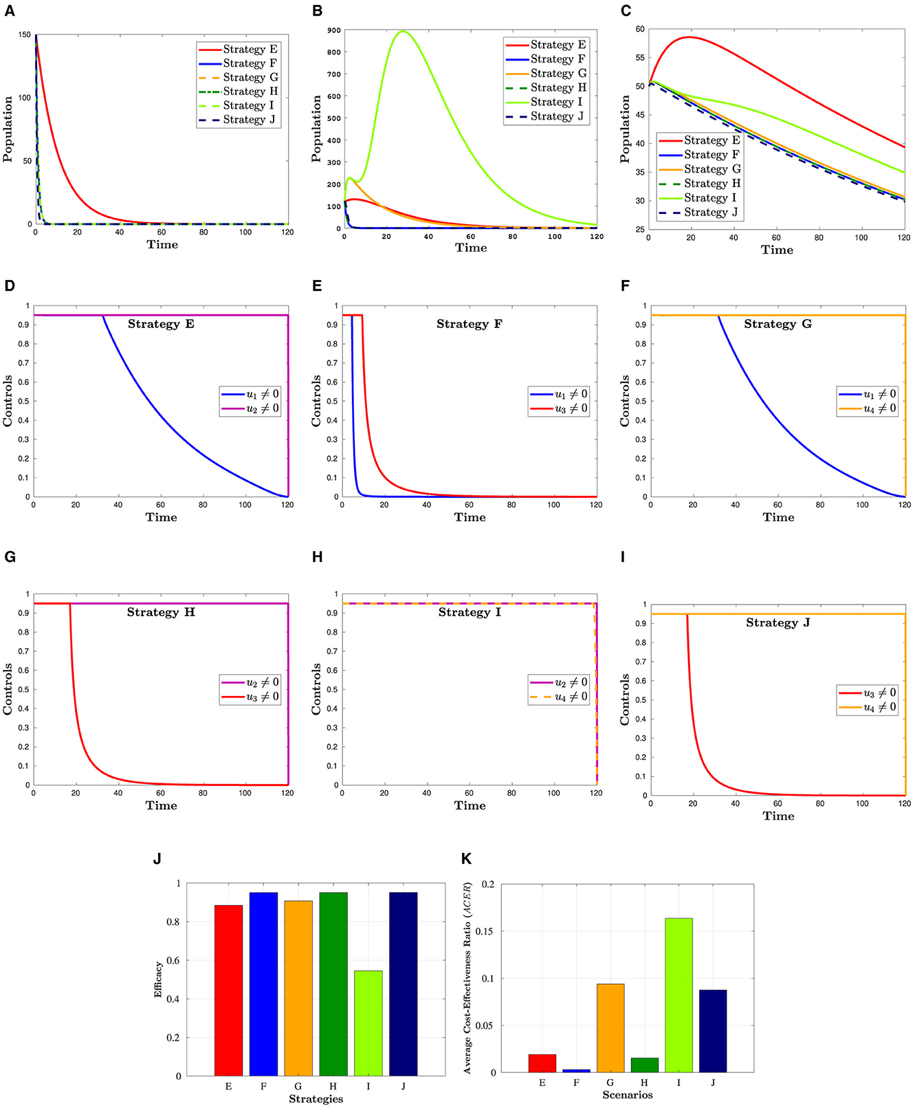
Figure 4. Simulation showing the effect strategies in Scenario 2. (A) H_c population. (B) $H_c^t$ population. (C) D_hc population. (D) Control profiles: u₁ and u₂. (E) Control profiles: u₁ and u₃. (F) Control profiles: u₁ and u₄. (G) Control profiles: u₂ and u₃. (H) Control profiles: u₂ and u₄. (I) Control profiles: u₃ and u₄. (J) Efficacy of strategies in scenario 2. (K) Cost-effectiveness of strategies in scenario 2.

5.2.3 Scenario 3: use of combinations of the controls

To investigate the impact of three control strategies, the following combinations are taken into account:

Strategy K: Combination of u₁, u₂ and u₃ (u₄ = 0)

Strategy L: Combination of u₁, u₂ and u₄ (u₃ = 0)

Strategy M: Combination of u₁, u₃ and u₄ (u₂ = 0)

Strategy N: Combination of u₂, u₃ and u₄ (u₁ = 0)

Figure 5 shows that a combination of three interventions is more successful in reducing the number of HIV and COVID-19 cases than using simply one or a hybrid of two strategies. Moreover, from this figure, we can see that H_c and D_hc populations appear to be reduced in almost the same manner in all four triple control strategies. The effectiveness of each of these strategies is demonstrated in Figure 5H, which was constructed using the information from Section 6.3. The corresponding control profiles are depicted in Figures 5D–G.

Figure 5

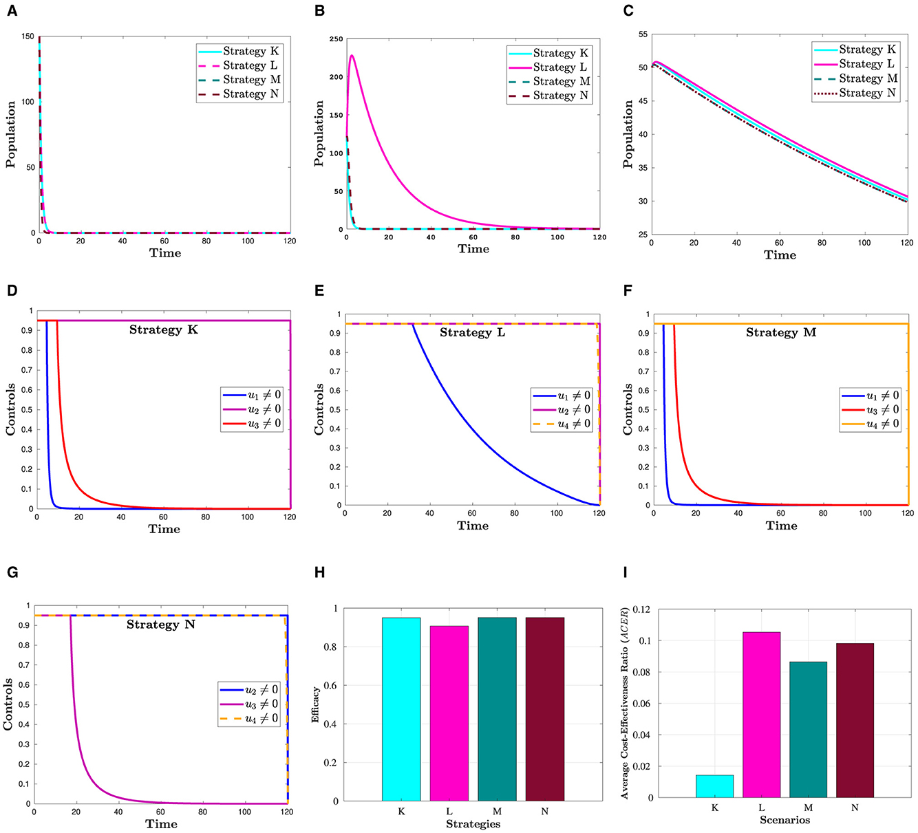
Figure 5. Simulation showing the effect strategies in Scenario 3. (A) H_c population. (B) $H_c^t$ population. (C) D_hc population. (D) Control profiles: u₁, u₂ and u₃. (E) Control profiles: u₁, u₂ and u₄. (F) Control profiles: u₁, u₃ and u₄. (G) Control profiles: u₂, u₃ and u₄. (H) Efficacy of strategies in scenario 3. (I) Cost-effectiveness of strategies in scenario 3.

5.2.4 Scenario 4: use of a combination of four control

This section refers to:

Strategy O: combination of u₁, u₂, u₃, and u₄.

Figure 6 reveals what happens when all control strategies are put into practice. This figure clearly indicates that applying all control measures is the most effective way to lessen the co-infection cases among all the intervention techniques included in this study.

Figure 6

Figure 6. Simulation showing the effect strategies in Scenario 4. (A) H_c population. (B) $H_c^t$ population. (C) D_hc population. (D) Control profiles: u₁, u₂, u₃, and u₄.

6 Cost-effectiveness analysis

In managing infectious diseases, it is important to identify an effective strategy that emphasizes favorable results while efficiently allocating resources. Effectiveness refers to the capacity to effectively control and mitigate the impact of diseases. For a variety of reasons, including financial constraints, it may not be feasible to rank the most effective options first, whereas the least expensive alternative may not have the desired effect. To create sustainable prevention strategies that maximize resources and promote the best possible health outcomes, it is imperative to strike a balance between effectiveness and costs. Cost-effectiveness aids in locating the optimal balance. Cost-effectiveness refers to resource allocation that maximizes the return on investment for the interventions made. Identifying effective and cost-effective strategies among the options provided in this study is the main objective of this section. Determining the most efficient and economical control strategy requires more analysis than simply comparing Figures 3–5, which shows the number of infected people at the end of the implementation of each strategy. The definitions and methodologies outlined in [42, 43] were used to conduct an efficacy and cost-effective analysis. Accordingly, effectiveness ($\tilde{E}$) is defined as the proportion of averted co-infection cases to the total number of possible co-infection cases under no intervention. That is,

$\begin{array}{ll}\tilde{E}=\frac{\text{Total averted co-infection cases }(T_{av})}{\text{The aggregate of co-infected in the course of }T\text{ period}}& (15)\end{array}$

The difference between the total number of individuals before and after the control techniques were implemented was used to calculate the overall number of co-infections avoided. In terms of effectiveness, the highest $\tilde{E}$ value is said to be the most effective, whereas the lowest $\tilde{E}$ value is said to be the least effective.

The infection-averted ratio (IAR), average cost-effectiveness ratio (ACER), and incremental cost-effectiveness ratio (ICER) are the three methods most frequently used in cost-effectiveness analyses. For this study, we considered the ACER and ICER methods. The following is the definition of ACER:

$\begin{array}{c}ACER=\\ \frac{\text{Total cost invested in a particular strategy }(T_{cost})}{\text{The aggregate of co-infections averted by the strategy }(T_{av})}.\end{array}$

The total cost was calculated using the cost function ${\int }_0^T\sum _{i=1}^4{Q}_i{u}_i(t)dt$. The ACER method evaluates the cost-effectiveness of a single intervention strategy by comparing it with the option of taking no action. This cost-effectiveness analysis method indicates that the best option is the one with the minimum ACER value.

The incremental cost-effectiveness ratio (ICER) is a method that enables the comparison of the health and cost benefits of two different interventions, which are vying for the same limited resources. When applying the ICER approach, it is important to compare two competing intervention strategies incrementally, with one intervention being compared to the next-less effective intervention. As a result, the control strategies are ranked according to the number of co-infections averted to examine the ICER of the strategies provided in scenarios 1, 2, 3, and 4, as shown in Table 2. Taking into account strategies m and n as two competing control measures, ICER is described as

$\begin{array}{l}ICER=\frac{\text{Change in total costs invested in strategies }m\text{ and }n}{\text{Change in the total number of co-infections averted in strategies }m\text{ and }n}.\end{array}$

Table 2

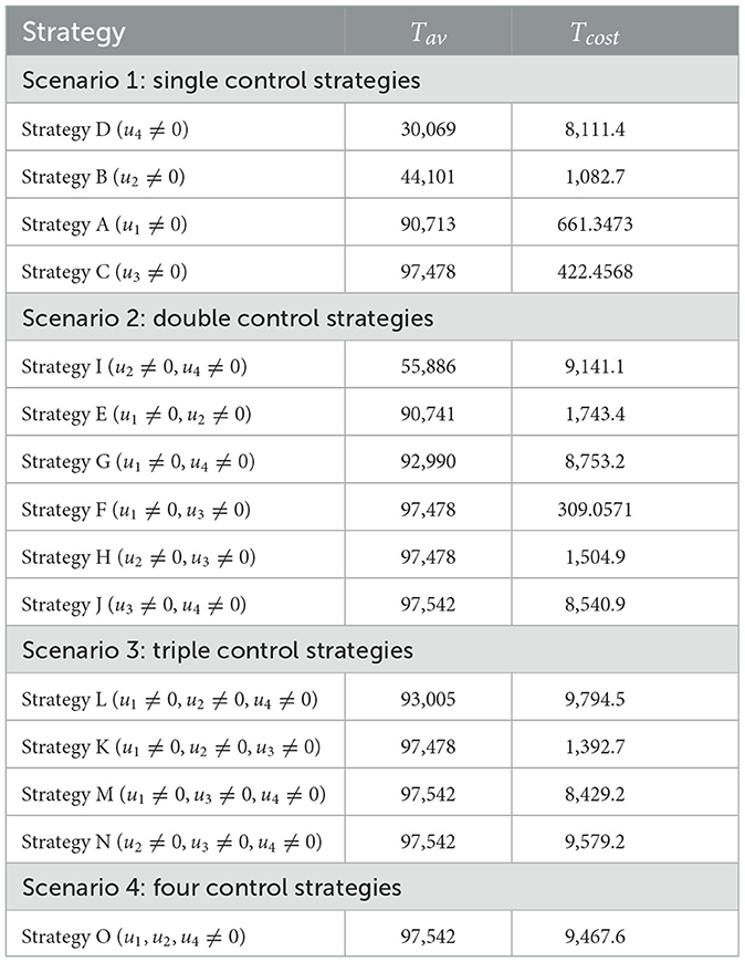
Table 2. Prevented co-infections and total cost of control strategies.

6.1 Cost-effectiveness analysis of scenario 1: single control strategy

We employ Equation 15 to calculate the effectiveness of the interventions. From Table 3, we can observe that Strategy C is the most effective among the strategies implemented in Scenario 2. Using ACER and ICER, we now look into the most economical approach. Following the definition and analysis of ACER, strategy D has the maximum ACER value, followed by strategies B, A, and C (see Table 3, fifth column). Consequently, this method suggests that Strategy C is the most economical in Scenario 1. Using the averted co-infection rank from Table 2, the ICER results, which are shown in Table 3, are calculated as follows:

$\begin{array}{lll}ICER(D)& =& \frac{8111.4-0}{30069-0}=0.2698\\ ICER(B)& =& \frac{1082.7-8111.4}{44101-30069}=-0.50091\\ ICER(A)& =& \frac{661.3473-1082.7}{90713-44101}=-0.00904\\ ICER(C)& =& \frac{422.4568-661.3473}{97478-9071390713}=-0.03531\end{array}$

Table 3

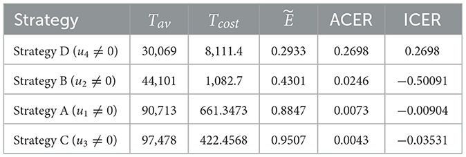
Table 3. T_av, T_cost, $\tilde{E}$, ACER, and ICER for the intervention strategies in Scenario 1.

When we compare ICER(D) and ICER(A), we find that approach A saves 0.2788 dollars in comparison with strategy D. Thus, strategy D is more costly than strategy A. Thus, in the next ICER computations, approach D is omitted. We will now carry on comparing the remaining three strategies.

$\begin{array}{lll}ICER(B)& =& \frac{1082.7-0}{44101-0}=0.02455\\ ICER(A)& =& \frac{661.3473-1082.7}{90713-44101}=-0.00904\\ ICER(C)& =& \frac{422.4568-661.3473}{97478-9071390713}=-0.03531\end{array}$

Upon examining the results, we can see that Strategy B is more expensive than Strategy A. Therefore, Strategy is ruled out since it is less cost-effective than Strategy A. The incremental cost-effectiveness ratio of strategies A and C is recalculated in the following manner:

$\begin{array}{lll}ICER(A)& =& \frac{661.3473-0}{90713-0}=0.00729\\ ICER(C)& =& \frac{422.4568-661.3473}{97478-9071390713}=-0.03531\end{array}$

Using strategy C results in a 0.0426 savings compared to strategy A. Therefore, of the four solutions in Scenario 1, strategy C is the most economical. This supports the outcome derived from the ACER analysis.

6.2 Cost-effectiveness analysis of scenario 2: combination of two control strategies

Although Strategy J is successful in preventing co-infections, based on the ACER value, the most economical approach among the options in scenario 2 is Strategy F, as shown in the fifth and sixth columns of Table 4. The ICER of the strategies in scenario 2 is determined using the rank of avoided co-infections shown in Table 4.

$\begin{array}{lll}ICER(I)& =& \frac{9141.1-0}{55886-0}=0.163567\\ ICER(E)& =& \frac{1743.4-9141}{90741-55886}=-0.21224\\ ICER(G)& =& \frac{8753.2-1743.4}{92990-90741}=3.11685\\ ICER(F)& =& \frac{309.06-8753.2}{97478-92990}=-1.88149\\ ICER(J)& =& \frac{8540.9-1509}{97542-97478}=109.9375\end{array}$

Table 4

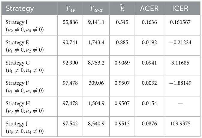
Table 4. T_av, T_cost, $\tilde{E}$, ACER, and ICER for the intervention strategies in Scenario 2.

It should be noted that ICER(H) is not determined in this case because Strategies F and H prevent the same number of co-infections. The remaining results, displayed in Table 4, indicate that ICER(G) is less than ICER(J). This implies that, because Strategy J is more expensive than Strategy G, it should be disregarded from the Scenario 2 options, even though it is more successful in preventing co-infections. Comparing the remaining strategies (E, F, G, H, and I), we can infer that Strategy G is pricier than Strategy I. Hence, it is also ruled out from further analysis. The ICER for each of the strategies I, E, and F is then computed as follows.

$\begin{array}{lll}ICER(I)& =& \frac{9141.1-0}{55886-0}=0.163567\\ ICER(E)& =& \frac{1743.4-9141}{90741-55886}=-0.21224\\ ICER(F)& =& \frac{309.06-1743.4}{97478-90741}=-0.21291\end{array}$

Comparing strategies E and I, it is evident that Strategy I dominates Strategy E. Consequently, Strategy I is omitted from the competitors in scenario 2. Next, as iterated below, the ICER is recalculated for Strategies E and F.

$\begin{array}{lll}ICER(E)& =& \frac{1743.4}{90741}=0.0192\\ ICER(F)& =& \frac{309.06-1743.4}{97478-90741}=-0.21291\end{array}$

The incremental cost-effectiveness ratio (ICER) values obtained for Strategy F indicate that Strategy E is overpriced and ineffective as compared to Strategy F. Afterward, Strategy E cannot be considered cost-effective in scenario 2. Consequently, we will continue to find a more cost-effective strategy from strategies F and H. It can be seen that although strategies F and H are the same in T_av, strategy F has a cost advantage over strategy H of 1, 054.9 − 309.06 = 1195.84. This affirms the cost-effectiveness of Strategy F. Based on this, we can conclude that Strategy F (promoting and delivering COVID-19 vaccines and treatments) is an economical approach offered in Scenario 2.

6.3 Cost-effectiveness analysis of scenario 3: combination of three control strategies

In Scenario 3, the effectiveness analysis shows that Strategies M and N are the most effective interventions (see Table 5). We performed an average cost-effectiveness ratio (ACER) analysis to determine the cost of applying the interventions and their effectiveness. From Table 5, we observe that Strategy K has the lowest ACER value. This value implies that Strategy K is an economical approach that can be implemented. To support this conclusion, we conducted an ICER analysis. The incremental cost-effectiveness ratio shown in Table 5 is calculated in the following manner:

$\begin{array}{lll}ICER(L)& =& \frac{9794.5-0}{93005-0}=0.10531\\ ICER(K)& =& \frac{1392.7-9794.5}{97478-93005}=-1.87834\\ ICER(M)& =& \frac{8429.2-1392.7}{97542-97478}=109.94531\end{array}$

Table 5

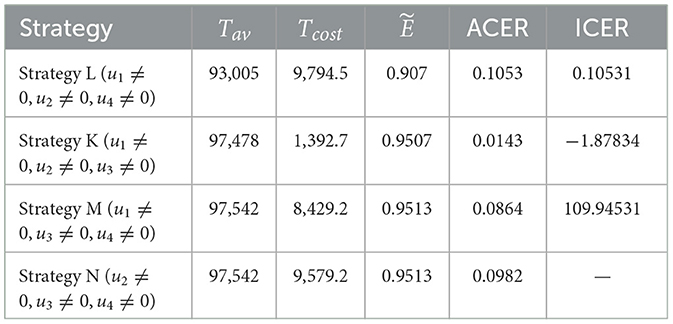
Table 5. T_av, T_cost, $\tilde{E}$, ACER, and ICER for the interventions in Scenario 3.

Note that because both Strategies M and N have the same T_av values, they prevent the same number of co-infections, ICER(N) is not computed here. A comparison of Strategies L and M shows that Strategy M strongly prevails over Strategy L. As a result, strategy M is excluded from further ICER analyses. We now compare Strategies L, K, and N.

$\begin{array}{lll}ICER(L)& =& \frac{9794.5-0}{93005-0}=0.10531\\ ICER(K)& =& \frac{1392.7-9794.5}{97478-93005}=-1.87834\\ ICER(N)& =& \frac{9579.2-1392.7}{97542-97478}=127.9141\end{array}$

Looking at the ICER values, we observe that Strategy N is overpriced than Strategy L. Therefore, Strategy N is ruled out. Further evidence that Strategy K is more affordable than Strategy L comes from comparing ICER(L) with ICER(K), which indicates a cost advantage of 1.9836 for Strategy K over L. Therefore, Strategy K (administering vaccines and treatments for COVID-19 and taking steps to prevent the spread of HIV) is the most economical among the four alternatives presented in Scenario 3.

6.4 Cost-effectiveness analysis of all scenarios

The effectiveness, ACER, and ICER analyses of the implementation of all control strategies (u₁, u₂, u₃, u₄ ≠ 0) are presented in Table 6. By comparing the effectiveness and costs of various strategies, we successfully identified the most efficient and cost-effective solutions for scenarios 1, 2, 3, and 4. Now, to identify the optimal approaches across all situations, we evaluate the most efficient strategies from each scenario and compare them. Table 7 displays the most cost-effective strategies for each scenario, which are ranked on the basis of the number of co-infections they have prevented. This table clarifies that Strategy O is the most effective in preventing co-infection cases as it successfully averted the highest number of co-infections compared to other strategies. Furthermore, according to the values indicated in the fifth column, Strategy F is the most economical approach among the given strategies across all scenarios. The ICER analyses further validate this conclusion, and they are conducted in the following manner:

$\begin{array}{lll}ICER(C)& =& \frac{422.4568-0}{97478-0}=0.0043\\ ICER(O)& =& \frac{946.6-422.4568}{97542-97478}=141.33\end{array}$

It is important to note that ICER(F) and ICER(K) cannot be calculated as both strategies have prevented the same number of cases, as indicated in Table 7. Accordingly, it is easy to see that Strategy O carries weight over Strategy C. As a result of this, strategy O is deemed unsuitable and therefore eliminated as an option. Comparing Strategies C, F, and K is still necessary. Despite preventing the same number of occurrences, Strategy F is the most economical, saving 422.4568 − 30906 = 113.4 compared to Strategy C and 1392.7 − 309.2 = 1083.642 in contrast with Strategy K. That is, Strategy F (promoting and delivering COVID-19 vaccines and treatments) is the most cost-effective among all the strategies provided in this study to tackle the challenges posed by HIV and COVID-19 co-infection, as shown in Figure 7. Therefore, it is recommended to prioritize these strategies for mitigating the impact of these diseases.

Table 6

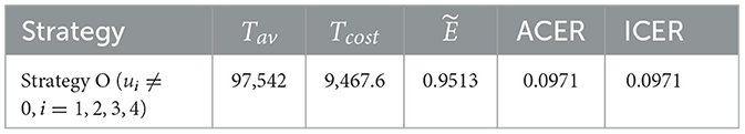
Table 6. T_av, T_cost, $\tilde{E}$, ACER, and ICER for the intervention strategies in Scenario 4.

Table 7

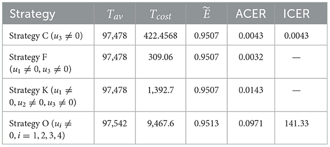
Table 7. Incremental cost-effectiveness ratio for scenarios 1–4.

Figure 7

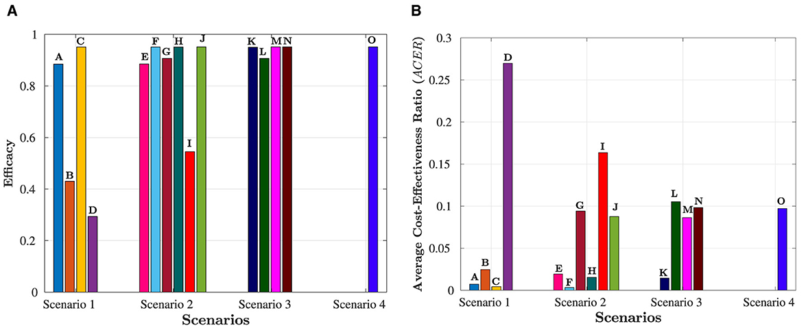
Figure 7. Overview of all scenarios and their comparative analysis. The letters at the top of the bars represent strategies in the scenario. (A) Efficacy of the four scenarios. (B) Cost-effectiveness of the four scenarios.

7 Discussion and conclusion

In this study, we introduce a deterministic model featuring nine distinct compartments: individuals susceptible to COVID-19, those who have received COVID-19 vaccination, individuals previously infected with COVID-19, individuals who have recovered from COVID-19, individuals with HIV, HIV-positive individuals undergoing treatment, individuals co-infected with HIV and COVID-19, HIV patients undergoing treatment and infected with COVID-19, and individuals at risk of dying as a result of co-infection. The well-posedness of the proposed model is established through the analysis of positivity, boundedness, existence, and uniqueness of its solutions. To investigate the co-infection dynamics, the model is divided into two sub-models: one for COVID-19 and another for HIV. Disease-free equilibria and basic reproduction numbers are determined to examine the system's behavior. It is observed that when the reproduction number for HIV $R_0^h<1$ is < 1, the HIV-free equilibrium point ($E_h^0$) becomes globally asymptotically stable, implying the eventual disappearance of the HIV-positive population. Conversely, the COVID-19 sub-model reveals a backward bifurcation phenomenon, where COVID-free ($E_c^0$)and endemic equilibrium ($E_c$) coexist, even when the reproduction number for COVID-19 $R_0^c<1$ is < 1. This epidemiological insight implies that merely reducing the reproduction number below one is insufficient to eradicate COVID-19 from the community. Furthermore, the study explores the impact of HIV on the spread of COVID-19 by examining the partial derivative of $R_0^c$ with respect to $R_0^h$. Under specific conditions, it is determined that HIV may contribute to the propagation of COVID-19. To address this co-infection burden, four control strategies are considered: HIV prevention, COVID-19 vaccinations, HIV treatment, and COVID-19 treatment. Optimal controls are characterized based on the Pontryagin minimum principle, offering a comprehensive framework for mitigating the impact of HIV and COVID-19 co-infection.

Numerical simulations are conducted to validate analytical findings and display the effectiveness of control strategies in mitigating HIV and COVID-19 co-infection scenarios. However, deciphering the cost-effectiveness of these strategies entirely through simulations proves challenging. Consequently, a comprehensive cost-effectiveness analysis, grounded in established theories, is executed to pinpoint the most economically viable strategy for curbing HIV and COVID-19 co-infections. Figures 3H, 4J, 5H, depict the efficacy of strategies in Scenarios 1, 2, and 3, respectively. Concurrently, the cost-effectiveness of these strategies is elucidated in the same figures. Overall, the analysis reveals that Strategy F, a synergistic approach involving COVID-19 vaccination and treatment, emerges as the most efficient and cost-effective strategy for diminishing the prevalence of co-infected individuals, as delineated in Figures 3H, 4J, 5H. These findings furnish valuable insights for policymakers, guiding them toward prioritizing preventive measures to reduce the incidence of co-infection cases and associated fatalities. Nevertheless, despite its significant contributions, it is imperative to acknowledge the study's limitations. Notably, the heightened susceptibility of HIV patients to new infections and their increased likelihood of transmitting the virus as the disease progresses remain unexplored in this study. This aspect represents an open area for further investigation, necessitating future research to incorporate the evolving impact of advanced HIV infection into the analytical framework.

Data availability statement

The original contributions presented in the study are included in the article/supplementary material, further inquiries can be directed to the corresponding author.

Author contributions

TB: Conceptualization, Formal analysis, Investigation, Methodology, Software, Validation, Visualization, Writing – original draft, Writing – review & editing. LO: Conceptualization, Formal analysis, Investigation, Supervision, Validation, Visualization, Writing – review & editing.

Funding

The author(s) declare that no financial support was received for the research, authorship, and/or publication of this article.

Conflict of interest

The authors declare that the research was conducted in the absence of any commercial or financial relationships that could be construed as a potential conflict of interest.

Publisher's note

All claims expressed in this article are solely those of the authors and do not necessarily represent those of their affiliated organizations, or those of the publisher, the editors and the reviewers. Any product that may be evaluated in this article, or claim that may be made by its manufacturer, is not guaranteed or endorsed by the publisher.

References

1. WHO. COVID-19 Dashboard. (2024). Available at: https://data.who.int/dashboards/covid19/deaths?n=o (accessed February 20, 2024).

Google Scholar

2. UNAIDS. The Path That Ends AIDS: UNAIDS Global AIDS Update. (2023). Available at: https://www.unaids.org/sites/default/files/media_asset/2023-unaids-global-aids-update_en.pdf (accessed May 19, 2024).

Google Scholar

3. WHO. Clinical Features and Prognostic Factors of COVID-19 in People Living With HIV Hospitalized With Suspected or Confirmed SARS-CoV-2 Infection, 15 July 2021. World Health Organization (2021).

Google Scholar

4. Danwang C, Noubiap JJ, Robert A, Yombi JC. Outcomes of patients with HIV and COVID-19 co-infection: a systematic review and meta-analysis. AIDS Res Ther. (2022) 19:1–12. doi: 10.1186/s12981-021-00427-y

PubMed Abstract | Crossref Full Text | Google Scholar

5. Kouhpayeh H, Ansari H. HIV infection and increased risk of COVID-19 mortality: a meta-analysis. Eur J Transl Myol. (2021) 31:10107. doi: 10.4081/ejtm.2021.10107

PubMed Abstract | Crossref Full Text | Google Scholar

6. Han X, Hou H, Xu J, Ren J, Li S, Wang Y, et al. Significant association between HIV infection and increased risk of COVID-19 mortality: a meta-analysis based on adjusted effect estimates. Clin Exp Med. (2022) 23:1–12. doi: 10.1007/s10238-022-00840-1

PubMed Abstract | Crossref Full Text | Google Scholar

7. Dong Y, Li Z, Ding S, Liu S, Tang Z, Jia L, et al. HIV infection and risk of COVID-19 mortality: a meta-analysis. Medicine. (2021) 100:26573. doi: 10.1097/MD.0000000000026573

PubMed Abstract | Crossref Full Text | Google Scholar

8. Episode 48: HIV and COVID-19. (2021). Available at: https://bit.ly/3wLbZqp (accessed October 14, 2024).

Google Scholar

9. WHO. Epidemiological Fact Sheet: HIV Statistics, Globally and by WHO Region. (2024). Available at: https://www.who.int/hiv/data/en/ (accessed February 20, 2024).

Google Scholar

10. Gatechompol S, Avihingsanon A, Putcharoen O, Ruxrungtham K, Kuritzkes DR. COVID-19 and HIV infection co-pandemics and their impact: a review of the literature. AIDS Res Ther. (2021) 18:1–9. doi: 10.1186/s12981-021-00335-1

PubMed Abstract | Crossref Full Text | Google Scholar

11. Bertagnolio S, Thwin SS, Silva R, Nagarajan S, Jassat W, Fowler R, et al. Clinical features of, and risk factors for, severe or fatal COVID-19 among people living with HIV admitted to hospital: analysis of data from the WHO Global Clinical Platform of COVID-19. Lancet HIV. (2022) 9:e486–95. doi: 10.1016/S2352-3018(22)00097-2

PubMed Abstract | Crossref Full Text | Google Scholar

12. Moyo E, Moyo P, Murewanhema G, Mhango M, Chitungo I, Dzinamarira T. Key populations and Sub-Saharan Africa's HIV response. Front Public Health. (2023) 11:1079990. doi: 10.3389/fpubh.2023.1079990

PubMed Abstract | Crossref Full Text | Google Scholar

13. Ringa N, Diagne M, Rwezaura H, Omame A, Tchoumi S, Tchuenche J. HIV and COVID-19 co-infection: a mathematical model and optimal control. Inf Med Unlock. (2022) 31:100978. doi: 10.1016/j.imu.2022.100978

PubMed Abstract | Crossref Full Text | Google Scholar

14. Omame A, Isah ME, Abbas M, Abdel-Aty AH, Onyenegecha CP, A. fractional order model for dual variants of COVID-19 and HIV co-infection via Atangana-Baleanu derivative. Alexand Eng J. (2022) 61:9715–31. doi: 10.1016/j.aej.2022.03.013

PubMed Abstract | Crossref Full Text | Google Scholar

15. Elaiw A, Al Agha A, Azoz S, Ramadan E. Global analysis of within-host SARS-CoV-2/HIV coinfection model with latency. Eur Phys J Plus. (2022) 137:1–22. doi: 10.1140/epjp/s13360-022-02387-2

PubMed Abstract | Crossref Full Text | Google Scholar

16. Batu TD, Obsu LL, Deressa CT. Co-infection dynamics of COVID-19 and HIV/AIDS. Sci Rep. (2023) 13:18437. doi: 10.1038/s41598-023-45520-6

PubMed Abstract | Crossref Full Text | Google Scholar

17. UNAIDS. Confronting Inequalities: Lessons for Pandemic Responses From 40 Years of AIDS. (2021). Available at: https://www.unaids.org/sites/default/files/media_asset/2021-global-aids-update_en.pdf (accessed July 1, 2024).

Google Scholar

18. Pal S, Kundu K, Chattopadhyay J. Role of standard incidence in an eco-epidemiological system: a mathematical study. Ecol Modell. (2006) 199:229–39. doi: 10.1016/j.ecolmodel.2006.05.030

Crossref Full Text | Google Scholar

19. Martcheva M. An Introduction to Mathematical Epidemiology. Vol. 61. New York, NY: Springer (2015).

Google Scholar

20. Li MY. An Introduction to Mathematical Modeling of Infectious Diseases. Mathematics of Planet Earth. Springer International Publishing (2018). doi: 10.1007/978-3-319-72122-4

Crossref Full Text | Google Scholar

21. Manfredi P, D'Onofrio A. Modeling the Interplay Between Human Behavior and the Spread of Infectious Diseases. New York, NY: Springer Science & Business Media (2013).

Google Scholar

22. Ashby B, Best A. Herd immunity. Curr Biol. (2021) 31:R174–7. doi: 10.1016/j.cub.2021.01.006

PubMed Abstract | Crossref Full Text | Google Scholar

23. Ogidi OI, Berefagha WL, Okara E. Covid-19 vaccination: the pros and cons. World J Biol Pharm Health Sci. (2021) 7:015–22. doi: 10.30574/wjbphs.2021.7.1.0072

Crossref Full Text | Google Scholar

24. WHO. Vaccine Efficacy, Effectiveness and Protection. (2024). Available at: https://www.who.int/news-room/feature-stories/detail/vaccine-efficacy-effectiveness-and-protection (accessed July 25, 2024).

Google Scholar

25. Klompas M. Understanding breakthrough infections following mRNA SARS-CoV-2 vaccination. JAMA. (2021) 326:2018–20. doi: 10.1001/jama.2021.19063

PubMed Abstract | Crossref Full Text | Google Scholar

26. Flacco ME, Acuti Martellucci C, Baccolini V, De Vito C, Renzi E, Villari P, et al. COVID-19 vaccines reduce the risk of SARS-CoV-2 reinfection and hospitalization: meta-analysis. Front Med. (2022) 9:1023507. doi: 10.3389/fmed.2022.1023507

PubMed Abstract | Crossref Full Text | Google Scholar

27. Höft MA, Burgers WA, Riou C. The immune response to SARS-CoV-2 in people with HIV. Cell Mol Immunol. (2024) 21:184-196. doi: 10.1038/s41423-023-01087-w

PubMed Abstract | Crossref Full Text | Google Scholar

28. Chukwu CW, Mushanyu J, Juga ML, Fatmawati. A mathematical model for co-dynamics of listeriosis and bacterial meningitis diseases. Commun Math Biol Neurosci. (2020) 2020:83. doi: 10.28919/cmbn/5060

Crossref Full Text | Google Scholar

29. Hale JK. Ordinary Differential Equations. New York, NY: Wiley (1969).

Google Scholar

30. Van den Driessche P, Watmough J. Reproduction numbers and sub-threshold endemic equilibria for compartmental models of disease transmission. Math Biosci. (2002) 180:29–48. doi: 10.1016/S0025-5564(02)00108-6

PubMed Abstract | Crossref Full Text | Google Scholar

31. WHO. Global Situation. (2024). Available at: https://covid19.who.int/ (accessed May 24, 2024).

Google Scholar

32. Chavez CC, Feng Z, Huang W. On the computation of $R_0$ and its role on global stability. Math Approach Emerg Reemerg Infect Dis. (2002) 125:31–65. doi: 10.1007/978-1-4757-3667-0_13

Crossref Full Text | Google Scholar

33. Castillo-Chavez C, Song B. Dynamical models of tuberculosis and their applications. Math Biosci Eng. (2004) 1:361. doi: 10.3934/mbe.2004.1.361

PubMed Abstract | Crossref Full Text | Google Scholar

34. Gumel AB. Causes of backward bifurcations in some epidemiological models. J Math Anal Appl. (2012) 395:355–65. doi: 10.1016/j.jmaa.2012.04.077

Crossref Full Text | Google Scholar

35. Deressa CT, Duressa GF. Modeling and optimal control analysis of transmission dynamics of COVID-19: the case of Ethiopia. Alexand Eng J. (2021) 60:719–32. doi: 10.1016/j.aej.2020.10.004

Crossref Full Text | Google Scholar

36. Mekonen KG, Balcha SF, Obsu LL, Hassen A. Mathematical modeling and analysis of TB and COVID-19 coinfection. J Appl Math. (2022) 2022:1–20. doi: 10.1155/2022/2449710

Crossref Full Text | Google Scholar

37. Fleming WH, Rishel RW. Deterministic and Stochastic Optimal Control. vol. 1 of Stochastic Modelling and Applied Probability. Springer-Verlag (1975).

Google Scholar

38. The World Bank. Population Ethiopia. (2022). Available at: https://data.worldbank.org/indicator/SP.POP.TOTL (accessed February 20, 2024).

Google Scholar

39. Ayele TK, Goufo EFD, Mugisha S. Mathematical modeling of HIV/AIDS with optimal control: a case study in Ethiopia. Results Phys. (2021) 26:104263. doi: 10.1016/j.rinp.2021.104263

Crossref Full Text | Google Scholar

40. Mekonen KG, Obsu LL, Habtemichael TG. Optimal control analysis for the coinfection of COVID-19 and TB. Arab J Basic Appl Sci. (2022) 29:175–92. doi: 10.1080/25765299.2022.2085445

Crossref Full Text | Google Scholar

41. Lenhart S, Workman JT. Optimal Control Applied to Biological Models. 1st ed. Chapman and Hall/CRC (2007).

Google Scholar

42. Darmawati D, Musafira M, Ekawati D, Nur W, Muhlis M, Azzahra SF. Sensitivity, optimal control, and cost-effectiveness analysis of intervention strategies of filariasis. Jambura J Math. (2022) 4:64–76. doi: 10.34312/jjom.v4i1.11766

PubMed Abstract | Crossref Full Text | Google Scholar

43. Rodrigues P, Silva CJ, Torres DF. Cost-effectiveness analysis of optimal control measures for tuberculosis. Bull Math Biol. (2014) 76:2627–45. doi: 10.1007/s11538-014-0028-6

PubMed Abstract | Crossref Full Text | Google Scholar