Emergence of chaotic resonance controlled by extremely weak feedback signals in neural systems

Introduction: Chaotic resonance is similar to stochastic resonance, which emerges from chaos as an internal dynamical fluctuation. In chaotic resonance, chaos-chaos intermittency (CCI), in which the chaotic orbits shift between the separated attractor regions, synchronizes with a weak input signal. Chaotic resonance exhibits higher sensitivity than stochastic resonance. However, engineering applications are difficult because adjusting the internal system parameters, especially of biological systems, to induce chaotic resonance from the outside environment is challenging. Moreover, several studies reported abnormal neural activity caused by CCI. Recently, our study proposed that the double-Gaussian-filtered reduced region of orbit (RRO) method (abbreviated as DG-RRO), using external feedback signals to generate chaotic resonance, could control CCI with a lower perturbation strength than the conventional RRO method.

Method: This study applied the DG-RRO method to a model which includes excitatory and inhibitory neuron populations in the frontal cortex as typical neural systems with CCI behavior.

Results and discussion: Our results reveal that DG-RRO can be applied to neural systems with extremely low perturbation but still maintain robust effectiveness compared to conventional RRO, even in noisy environments.

1 Introduction

Over the current decade, the mechanism of stochastic resonance where synchronization against a weak input signal is enhanced by additive stochastic noise has been applied to many engineering fields [1–3], especially the biomedical field [4–7] including validation in neural models [8, 9] [reviewed in [10, 11]]. Moreover, recent studies have demonstrated that chaotic behaviors in neurons can significantly impact neural dynamics, influencing the firing rates and latency of neuronal responses [12]. Not restricting additive stochastic noise, chaos as internal dynamic fluctuations also cause a similar phenomenon to stochastic resonance, which is referred to chaotic resonance [reviewed in [13–15]]. Chaotic resonance exhibits higher sensitivity than stochastic resonance [16, 17]; therefore, there is a need to develop engineering applications to utilize this advantage [reviewed in [15, 18]].

Several chaotic resonance types have been previously observed [reviewed in [15]]. The first type is chaotic resonance in excitable systems represented by the spiking neural system [19–23]. In this chaotic resonance type, the chaotic spikes for each trial respond at various points against the repeated input signal, unlike the periodic spikes that respond at specific timings. Consequently, the spike distribution converges on the shape of the input signal [19–23]. In addition, autaptic connections have been found to modulate chaotic resonance, enhancing or altering its characteristics depending on the type of autapse and its parameters [24]. The second type is chaotic resonance with chaos–chaos intermittency (CCI), where the chaotic orbits shift between the separated chaotic attractor regions, such as the cubic map, Chua's circuit, and excitatory–inhibitory (E-I) system [25, 26]. The return map inducing this type of chaotic resonance has the shape of a cubic function. Under the attractor-separated condition, the small absolute values of local extremes in the return map function lead to the trapped orbit in specific regions. While under the attractor-merging condition, the orbit can jump between specific regions, and CCI occurs due to the increasing absolute value of local extremes in the return map function. Around the attractor-merging bifurcation point, the inherent shift between chaotic attractor regions rarely occurs in the systems. In this condition, applying an external signal induces an effect that causes the orbit to shift among the attractor regions. Consequently, CCI synchronizes with the input signal despite its significantly weak strength [16, 17, 25, 27, 28]. Recent studies for engineering applications have been proceeding against the latter type of chaotic resonance [reviewed in [15, 18]]. Conventionally, controlling chaotic resonance requires the internal order parameters to be adjusted [25, 26]. However, in many systems, especially biological systems, adjusting the internal order parameters from the outside environment is challenging.

To understand the dynamics of neural populations, some models illustrate how chaotic activity emerges from the interactions within excitatory–inhibitory neural networks [29]. Despite simplification, Hadaeghi's and Baghdadi's models [30, 31] offer valuable insights into the dynamic interactions between excitatory and inhibitory neurons, contributing to our understanding of neurological disorders such as bipolar disorder (BD) and attention deficit hyperactivity disorder (ADHD), respectively. Those models can be used as valuable tools for investigating the broader principles of neural dynamics and the potential implications of chaos control methods in neural systems. Conventionally, to apply chaotic resonance with CCI, the attractor-merging bifurcation must be controlled by the internal parameters [reviewed in [25, 26]]. Furthermore, the application of chaotic resonance in neural systems has been explored in various contexts, showing that chaotic signals can enhance the detection of weak signals and improve neural network performance [32]. However, the reduced region of orbit (RRO) method has emerged as an approach [33] to control chaotic resonance with CCI by external feedback signals. By utilizing external feedback signals, the RRO method offers a novel means of modulating chaotic dynamics, circumventing the challenges associated with conventional parameter adjustments [26]. This methodological innovation has sparked interest in its potential applications across various domains, particularly in the treatment of neurological disorders, where precise control over neural dynamics is difficult [34, 35]. Despite achieving CCI control using weak external feedback signals, the conventional RRO method still faces limitations with systems that desire weaker perturbations. In particular, to induce CCI with a weak feedback signal, the profile of the feedback signal must be concentrated around the local extremes of the map function, referred to as the local specification. However, the profile used in the conventional RRO method is insufficient. Recently, our proposed method, the double Gaussian-filtered RRO (DG-RRO) method [36], controls CCI with a lower perturbation strength than the conventional RRO method by the effect of high local specification. Accordingly, the DG-RRO feedback signal induces chaotic resonance with extremely weak feedback perturbation [36]. By utilizing external feedback signals, the DG-RRO method might offer a potential avenue for neuro-feedback applications, allowing for the precise modulation of neural dynamics.

The previous study had drawbacks in experimenting with the DG-RRO method. Iinuma et al. only applied the DG-RRO method in discrete cubic maps, not with neural systems. Therefore, the evaluation of more physiological conditions is needed to validate the effectiveness of the DG-RRO method in experimental systems, specifically in neural systems, which is the primary applied system with the RRO method [34, 35]. Furthermore, the effect of noise on this method is also considered since the presence of noise in actual systems is inevitable. Previous studies which evaluated the conventional RRO method investigated the influence of two primary sources of noise [37], namely, background noise [13, 14, 38] (referred to as the additive noise in this study) and measurement error [25, 34] (referred to as the contaminant noise in this study). In particular, additive noise mainly exists in the internal system and affects the neural system, while contaminant noise exists in the measurement environment [37].

In this context, this study aims to validate that the CCI produced by the DG-RRO feedback signal can be applied to neural systems and maintain robustness even in the presence of noise. More concretely, in our previous study [36], we applied DG-RRO to abstract cubic maps. Building upon this groundwork, in this study, we evaluated the application of the DG-RRO method on the excitatory–inhibitory neural system model as typical neural systems with CCI behavior compared with the conventional RRO method. Furthermore, we investigated the influence of two types of noise (additive and contaminant noise) on those neural models.

2 Materials and methods

2.1 Neural system composed of the frontal and sensory cortices

The model used in this research, inspired by the Hadaeghi [30] and Baghdadi models [31], is a mathematics model, which emphasizes the imbalance between excitatory and inhibitory neuron populations in the frontal cortex [39, 40], and crucial for reproducing neural activities. Moreover, it highlights dysfunction in feedback loops from the sensory cortex to the frontal cortex, alongside abnormal temporal behavior of attention levels originating from frontal cortex imbalance [31]. All variables and parameters used in this model are dimensionless to suit the research purposes. The neural activity of the frontal cortex is depicted as x(n)(n = 1, 2, ...), regulated by the interaction between excitatory and inhibitory neural populations. Figure 1 provides an overview of the model as follows:

$\begin{array}{ll}x(n+1)=F(x(n)),& (1)\end{array}$

$\begin{array}{ll}F(x)=C(Btanh({\omega }_{2}x)-Atanh({\omega }_{1}x)),& (2)\end{array}$

where F(x) represents the map function for x(n). ω₁ and ω₂ are the synaptic weights of inputs to the inhibitory and excitatory neural populations, respectively. A and B correspond to the synaptic weights of the outputs of the inhibitory and excitatory neural populations, respectively. In Equation (2), C is an attenuation coefficient of frontal neural activity. In this model, frontal neural dynamics x(n) is determined by output from the frontal cortex and its feedback through the sensory cortex with attenuation C. The setting of C < 1.0 corresponds to the case of the loss of information of brain activity due to lower attention [31]. The parameters used in this study are set as follows: ω₁ = 0.2223, ω₂ = 1.487, and B = 5.82, and A is the main bifurcation parameter based on the previous studies of the Hadaeghi [30, 41] and the Baghdadi models [31]. The Hadaeghi model with only the frontal cortex component is a special case of the Baghdadi model with the attenuation coefficient C = 1.0, while the Baghdadi model has an attenuation coefficient C ≤ 1.0. CCI is induced when C ≳ 0.85; therefore, in this study, we used C = 0.9 as the represented parameter to produce abnormal frontal cortical neural activity [35].

Figure 1

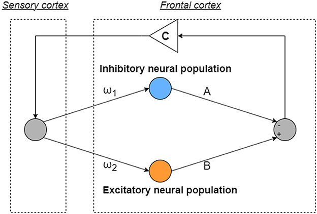
Figure 1. Overview of neural systems composed of the frontal and sensory cortices to reproduce healthy and abnormal neural activity. ω₁ and ω₂ are the synaptic weights of inputs to the inhibitory and excitatory neural populations, respectively. A and B correspond to the synaptic weights of the outputs of the inhibitory and excitatory neural populations, respectively. C is an attenuation coefficient which is feedback from output from the frontal cortex going through to the sensory cortex.

The behavior of the neural system composed of the frontal and sensory cortices, including the bifurcation diagram of the frontal neural activity x(n) and F(f_min)/ F(f_max), as shown in Figure 2A. The attractor-merging condition in case of no feedback signal is defined as [33] F(f_max) < 0, F(f_min) > 0, where f_max and f_min are the local maximum and minimum of the map function, and CCI occurs when A ≳ 9.8. In 12.5 ≲ A ≲ 13.5, frontal neural activity is in the periodic state corresponding to CCI of patients with BD achieving a healthy periodic state (healthy control [HC]). Figure 2B illustrates an example of the frontal neural activity x(n) in HC (A = 13) and in patients with disturbance (A = 12) [34], where they both satisfied the attractor-merging condition.

Figure 2

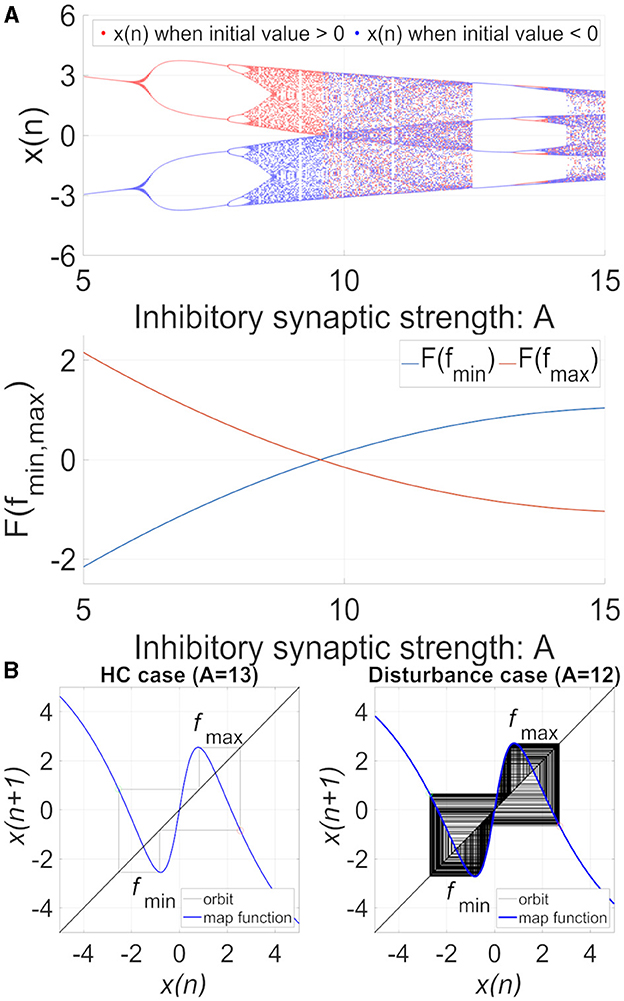
Figure 2. (A) System behaviors in the neural network comprised the frontal and sensory cortices in the model with C = 1.0 as a function of the synaptic weight from the inhibitory neural population, A, in the absence of feedback and periodic signals (K = 0, A_s = 0). (Top) Bifurcation diagram of the frontal neural activity x(n) represented by Equation (1) as a function of A blue and red dots indicate positive and negative initial values of x(0), respectively. (Bottom) F(f_min)/ F(f_max) as a function of A. The frontal neural behavior in the periodic window 12.5 ≤ A ≤ 13.5 corresponds to that of healthy controls (HC). In comparison, the CCI behavior in 9.8 ≤ A ≤ 12.5 and A ≥ 13.5 corresponds to that of patients with disturbance. (B) Map function F(x) (the orbit in the return map) of frontal cortical neural activity x(n) in the absence of external feedback or periodic input signals (K = 0, A_s = 0). HC case (weight from the inhibitory neural population is (A = 13.0) (left) and disturbance case (A = 12.0) (right). In the return maps, the red and green circles indicate F(f_max) and F(f_min), respectively. In both HC and disturbance, the attractor-merging condition is satisfied with F(f_max) < 0 and F(f_min) > 0; the periodic and CCI states correspond to HC and disturbance, respectively.

2.2 Controlling frontal cortical neural activity by RRO feedback

In this model, the healthy and disturbed states are produced by a period state and a CCI state in the frontal cortical neural activity, respectively. In addition, the enhancement of the neural pathway corresponds to increasing the strength of neural pathway C from the sensory cortex to the frontal cortex. In previous studies, RRO feedback signals were applied to induce chaotic resonance to transition the CCI of x(n) to the period state [34, 35]. An overview of the systems for this control method is presented in Figure 3. The frontal cortical neural activity x(n) is controlled by feedback signals and a periodic input signal S(n) = A_s sin(Ωn) corresponding to the external treatment signal [34, 35] as follows:

$\begin{array}{ll}x(n+1)=F(x(n))+Ku(x(n))+S(n),& (3)\end{array}$

$\begin{array}{ll}u(x)=-(x-x_d)exp(-{(x-x_d)}^2/(2{\sigma }^2)).& (4)\end{array}$

where K, x_d, and σ represent the RRO feedback strength, the merging point of two chaotic attractors, and a parameter to determine the region of the RRO feedback effect, respectively. F(x) is the map function. In previous studies, x_d = 0 and σ = 1.0 were set [34, 35] because the structure of the return map of Equation (2) has a point symmetry at approximately x = 0 with local maximum and minimum values of the map function located within the region -σ < x < σ (σ = 1.0) [33].

Figure 3

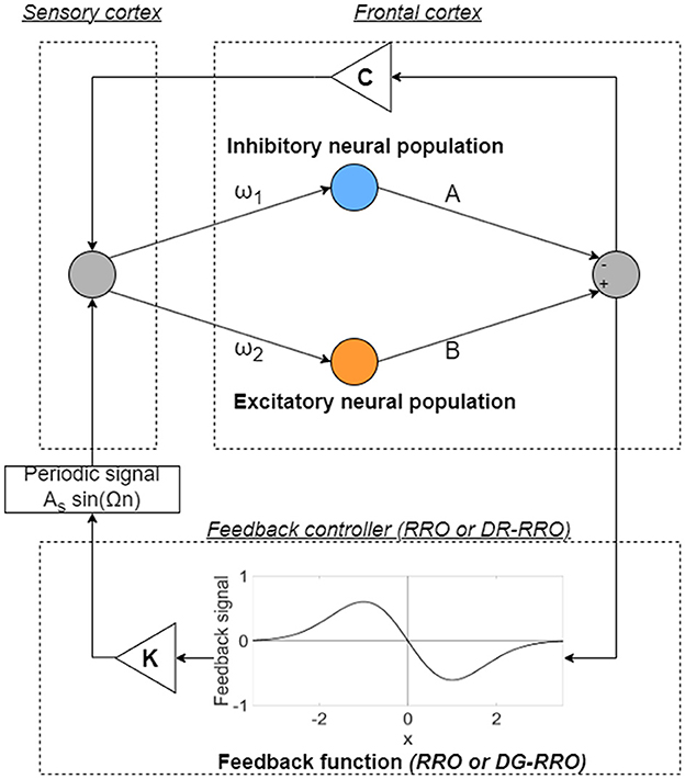
Figure 3. Overview of the neural system with the feedback signals [reduced region of orbit (RRO) or double Gaussian-filtered RRO (DG-RRO) feedback signal]. The neural systems composed of the frontal and sensory cortices reproduce the neural activity. The frontal cortical neural activity x(n) is controlled by feedback signals (RRO or DG-RRO) and a periodic input signal S(n) = A_s sin(Ωn).

Figure 4 shows the map function of Equations (3, 4) in the case of the presence and absence of RRO feedback signals in the model with C = 1.0, to illustrate the effect of the RRO. The attractor merging (CCI) with feedback signal occurs if it satisfies the attractor-merging condition (F(f_max) + Ku(f_max) < 0, F(f_min) + Ku(f_min) > 0). For an inhibitory synaptic weight A = 12.0 in the absence of feedback (K = 0), the attractor-merging conditions are satisfied (left graph in Figure 4). The orbit x(n) hops between positive and negative x regions, i.e., CCI arises. With positive feedback (K = 0.7 and A = 12.0 case), the absolute values of f_max and f_min are reduced, and the attractor merging conditions are not satisfied; the orbit x(n) is constrained to lie within either the positive or negative x region, depending on the initial value of x(0).

Figure 4

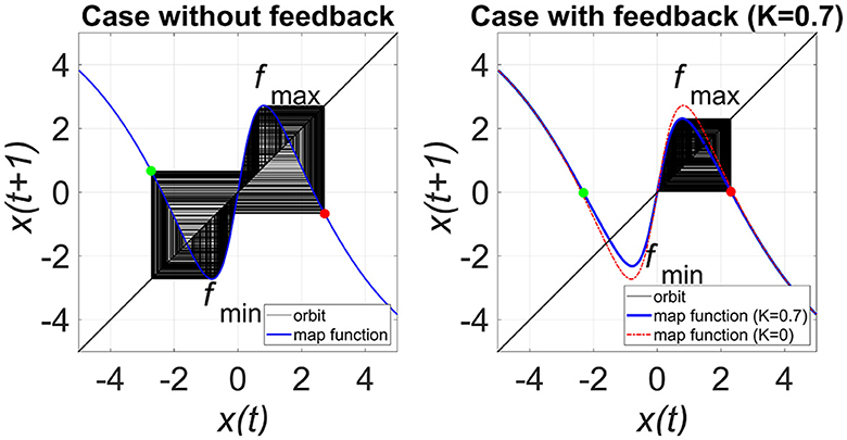
Figure 4. Map function F(x) + Ku(x) for A = 12.0 with and without external feedback signals in the return map between x(n) and x(n + 1) in the model with C = 1.0. The left and right graphs indicate map functions satisfying attractor-merging conditions with K = 0.0 and not satisfying attractor-merging conditions with and K = 0.7 in the A = 12.0 case. The red and green dots indicate F(f_max) + Ku(f_max) and F(f_min) + Ku(f_min), respectively. RRO feedback separates the merged attractors by decreasing the absolute values of f_max and f_min.

2.3 Controlling frontal cortical neural activity by DG-RRO feedback

The RRO feedback signal presented in Equation (4) consists of a linear function −(x−x_d) that can adjust the local maximum and minimum values of the map function F(x) and a single Gaussian function around the attractor dividing point x_d, as shown in the upper part of Figure 5. The figure was obtained based on the parameter set from the previous study (σ = 1.0, x_d = 0). However, the local specification at approximately x = x_min (x_min:f_min = F(x_min)) and x = x_max (x_max:f_max = F(x_max)), which is the degree for rapidly converging to zero from x = x_{min, max} in the feedback signals, can be improved. To achieve this improvement, DG-RRO feedback signals g(x) proposed by Iinuma et al. [36] used a reversal function −F(x) and double Gaussian functions at approximately x = x_{min, max} as follows:

$\begin{array}{c}x(n+1)=F(x(n))+Kg(x(n))+S(n),\\ g(x)=-F(x)\left[exp(-{(x-x_{\text{min}})}^2/(2{\sigma }_{\text{dg}}^2))+exp(-{(x-x_{\text{max}})}^2/(2{\sigma }_{\text{dg}}^2))\right],& (5)\end{array}$

where σ_dg is a parameter related to the influence range of the feedback signal. In this study, σ_dg was set as σ_dg = σ/2 = 0.5. The lower part of Figure 5 shows the profile of DG-RRO feedback signal g(x). Compared with the RRO feedback signal, g(x) converges rapidly to zero except at approximately x = x_{min, max}; that is, a higher local specification around local minimum and maximum points is achieved using the DG-RRO method. Like the conventional RRO method, the DG-RRO method decreases the absolute value of f_min and f_max. By adjusting the feedback signal strength K for approaching attractor-merging bifurcation (F(f_min) + Kg(f_min) = 0 and F(f_max) + Kg(f_max) = 0), the inherent shift between the positive and negative regions of x(n) rarely occurs in the systems. Under this condition, applying an external signal induces an effect that causes the orbit shift among the attractor regions. Consequently, CCI synchronizes with the input signal despite its significantly weak strength. However, unlike the conventional RRO method, the DG-RRO feedback signal modifies the dynamics more effectively by using these double Gaussian functions, ensuring that the feedback influences are more focused at the local minimal and maximal points and improving the efficiency of this control method by using smaller feedback strength.

Figure 5

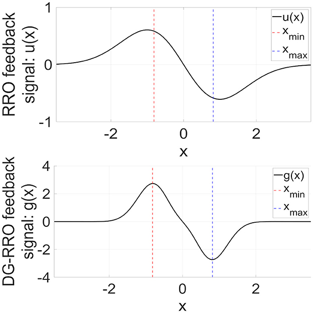
Figure 5. (Upper part) RRO feedback signal u(x) given by Equation (4). (Lower part) Double Gaussian RRO (DG-RRO) feedback signal g(x) given by Equation (5) in the model with C = 1.0. The local minimum (x_min)/maximum (x_max) points for map function F(x) given by Equation (2). Weight from the inhibitory neural population A = 12.0. Compared with the RRO feedback signal, g(x) rapidly converges to zero except for approximately x = x_min, x_max; that is, higher local specification around local minimum/maximum points achieved by the DG-RRO method.

In actual systems, noise is inevitable and may affect CCI. In this study, to appraise the influence of noise on chaotic resonance, in addition to DG-RRO feedback signals, the additive and contaminant noise [37] were applied to the DG-RRO feedback signals. After applying the noise, the overall system dynamics are expressed as follows:

$\begin{array}{l}x(n+1)=F(x(n))+Kg(x(n)+D_c\eta (n))+D_a\xi (n)+S(n),\end{array}$

where η and ξ represent the Gaussian white noise (random signal with a mean value of 0 and standard deviation of 1). D_a and D_c denote the strength of additive stochastic and contaminant noise, respectively. Our previous study on the types of noise influence on system dynamics degraded the synchronization in chaotic resonance [37]. Additive noise perturbs the system directly by introducing random fluctuations to the input signal. In contrast, contaminant noise affects neural activity through feedback function, which means the contaminant noise passively affects the system by changing the feedback signal. With significant contaminant noise, feedback terms behave as noise unrelated to neural activity. Therefore, contaminant noise exhibits a similar effect to additive noise [37].

2.4 Evaluation indices

The attractor-merging condition for the RRO and DG-RRO feedback signal was applied to determine the attractor-merging bifurcation point. We described the attractor-merging bifurcation point F(f_min) + Ku(f_min) = 0 and F(f_max) + Ku(f_max) = 0 for the RRO method and F(f_min) + Kg(f_min) = 0 and F(f_max) + Kg(f_max) = 0 for the DG-RRO method. When F(f_max) + Ku(f_max) < 0 and F(f_min) + Ku(f_min) > 0 for the RRO case, F(f_max) + Kg(f_max) < 0 and F(f_min) + Kg(f_min) > 0 for the DG-RRO case, it called attractor-merging condition [33]. Otherwise, it is called the attractor-separating condition.

To evaluate the amount of perturbation due to the feedback signal (e.g., Kg(x)), the perturbation for the DG-RRO method is calculated as follows:

$\begin{array}{l}\text{Θ}=<{(Kg(x(n)))}^2+S{(n)}^2>,\end{array}$

and the perturbation for the RRO method is calculated as follows:

$\begin{array}{l}\text{Θ}=<{(Ku(x(n)))}^2+S{(n)}^2>,\end{array}$

where 〈·〉 denotes the average in n [34]. The values for Θ are measured against 10 trials with different initial conditions of x(0).

The synchronization between x(n) and S(n) was evaluated by using their correlation coefficient at a time delay τ as follows:

$\begin{array}{c}\text{Corr}(\tau )=\frac{C_{sx}(\tau )}{\sqrt{C_{ss}{C}_{xx}}},\\ C_{sx}(\tau )=\langle (S(n+\tau )-\langle S\rangle )(X(n)-\langle X\rangle )\rangle ,\\ C_{ss}(\tau )=\langle {(S(n)-\langle S\rangle )}^2\rangle ,\end{array}$

$\begin{array}{c}{C}_{xx}(\tau )=\langle {(X(n)-\langle X\rangle )}^2\rangle ,\end{array}$

where 〈·〉 denotes the average in n. X represents the binarised x(n) value, i.e., X(n) = 1 in x(n)≥0 case and X(n) = −1 in x(n) < 0 case in order to focus on the CCI behavior. In this study, τ was set to the value for $arg{max}_{\tau }\mathrm{\text{Corr}}(\tau )$ in each time series of x(n). The values for $arg{max}_{\tau }\mathrm{\text{Corr}}(\tau )$ are measured by different τ values and average against 10 trials with different initial values of x(0).

3 Results

3.1 Frontal cortical neural activity behaviors under the influence of external feedback signal

We demonstrated the dependency of frontal cortical neural activity x(n) on the feedback strength K in the case of conventional RRO and DG-RRO methods to control CCI in noise-free conditions (D_a = 0, D_c = 0). Figure 6 shows the bifurcation diagram and perturbation Θ when the applied feedback signals are the RRO and DG-RRO methods in the case of C = 1.0 (see Figure 6A) and in the case of C = 0.9 (see Figure 6B) (frequency Ω = 0.005 is set). The results revealed that the strengths of feedback signals K, where the chaotic attractor achieved the attractor-merging bifurcation (F(f_min)+Ku(f_min) = 0, and F(f_max)+Ku(f_max) = 0, F(f_min)+Kg(f_min) = 0, and F(f_max)+Kg(f_max) = 0) are K≈0.68 for the RRO method and K≈0.13 for the DG-RRO method when C = 1.0 and K≈0.28 for the RRO method and K≈0.06 for the DG-RRO method when C = 0.9. Owing to the better local specification (see Figure 5), the DG-RRO method required significantly smaller perturbation Θ than the conventional RRO method to achieve the attractor-merging bifurcation; thus, the amount of the perturbation for the DG-RRO method was two-ninth of the amount of the perturbation for the RRO method (Θ≈0.017 for the DG-RRO method and Θ≈0.075 for the RRO method when C = 1.0, and Θ≈0.0089 for the DG-RRO method, Θ≈0.04 for the RRO method when C = 0.9) (see bottom parts of Figure 6). To easily compare perturbation Θ at attractor-merging bifurcation points of each method, Figure 6C shows the perturbation values of both methods at C = 1.0 and C = 0.9 cases.

Figure 6

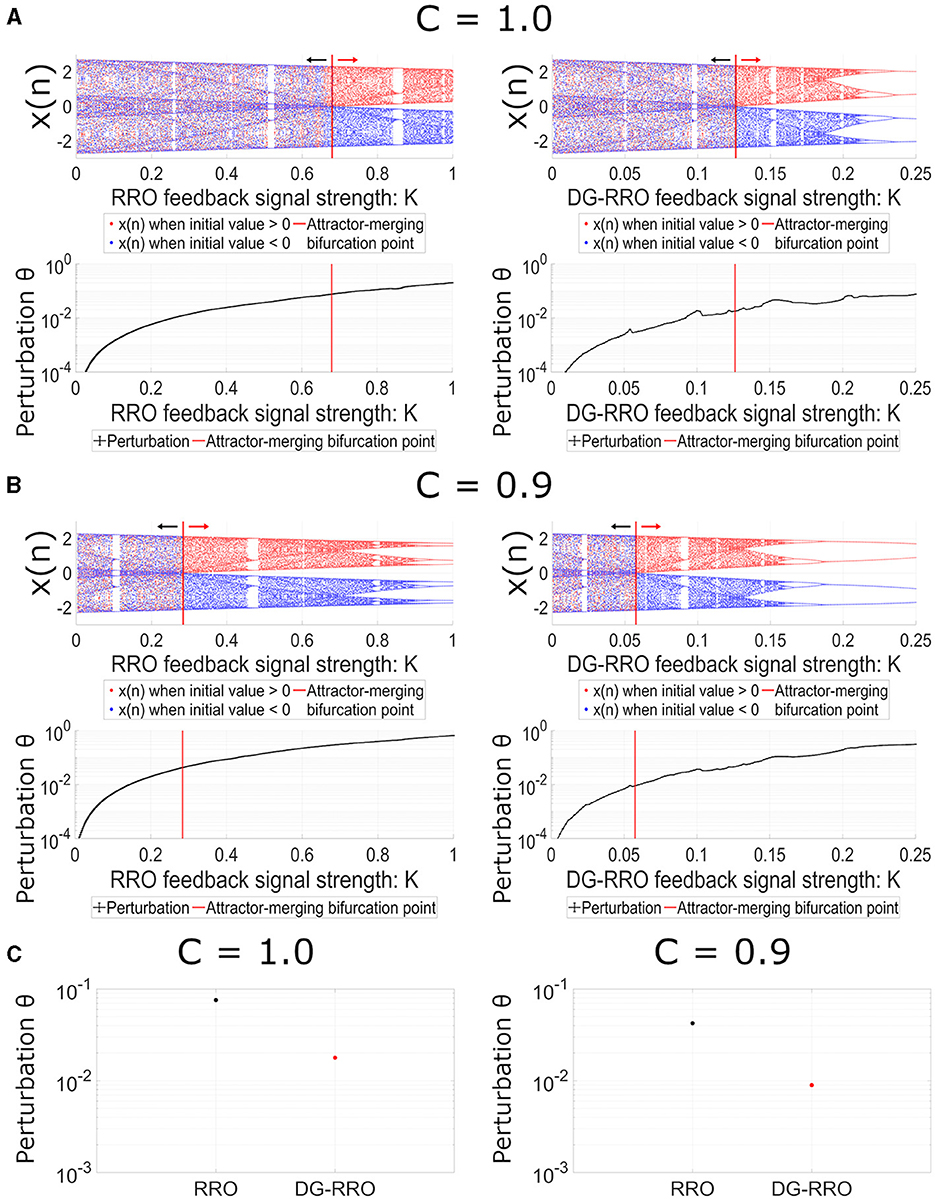
Figure 6. Dependence of system behavior on RRO (left) and DG-RRO (right) feedback strength K (A) when C = 1.0 and (B) when C = 0.9 (B = 13.0, ω₁ = 0.2223, ω₂ = 1.487, A_x = 0.01, Ω = 0.005). The red solid line indicates the feedback strength K where attractor merging bifurcation F(f_min) + Ku(f_min) = 0 and F(f_max) + Ku(f_max) = 0, F(f_min) + Kg(f_min) = 0, F(f_max) + Kg(f_max) = 0 arises. (Top) The bifurcation diagram of frontal neural activity. The black arrows point to the attractor-separating condition (F(f_min) + Ku(f_min) < 0, F(f_max) + Ku(f_max) > 0/ F(f_min) + Kg(f_min) < 0, F(f_max) + Kg(f_max) > 0) regions; the red arrows point to the attractor-merging condition (F(f_min) + Ku(f_min) > 0, F(f_max) + Ku(f_max) < 0/F(f_min) + Kg(f_min) > 0, F(f_max) + Kg(f_max) < 0) regions. (Bottom) Dependence of perturbation Θ on the strength of feedback signals K. (C) Comparison of perturbation between the RRO and DG-RRO method at attractor merging bifurcation.

3.2 Controlling signal response of the frontal cortical neural activity with the DG-RRO method

We evaluated the sensitivity of the DG-RRO method according to feedback strength K under chaotic resonance and compared it with the conventional RRO method in noise-free conditions (D_a = 0, D_c = 0). Figure 7 illustrates the correlation coefficient arg max_τCorr(τ) according to feedback strength K and input signal strength A_s (frequency Ω = 0.005 is set). When the periodic signal strength is large (A_s≈1), this periodic signal S(n) dominates and leads to high correlation regardless of the influence of the feedback signal. However, when the input strength A_s values are smaller, the high correlation only occurs near the attractor-merging bifurcation. Accordingly, around this value of feedback strength, CCI reaches higher synchronization with the input signals S(n) than other feedback signal strength ranges, i.e., higher sensitivity is achieved. In particular, regarding the comparison between the DG-RRO and RRO methods, Figure 8 shows the arg max_τCorr(τ) at the attractor-merging bifurcation according to the feedback signal strength K and input signal strength A_s in noise-free conditions (D_a = 0, D_c = 0) (frequency Ω = 0.005 is set). As observed in Figure 8, the arg max_τCorr(τ) decreases with weaker input strength. However, within $10^{-4}\le A_s\le 5\times 10^{-2}$ when C = 1.0 and $10^{-4}\le A_s\le 10^{-2}$ when C = 0.9, the arg max_τCorr(τ) of the DG-RRO method is superior to that in the RRO method. Moreover, the DG-RRO method maintains a high correlation (arg max_τCorr(τ) > 0.7) for $2\times 10^{-3}\lesssim A_s\le 10^{-1}$ when C = 1.0 and for $10^{-3}\lesssim A_s\le 10^{-1}$ when C = 0.9. In comparison, the high correlation of the RRO method is only maintained for $4\times 10^{-2}\lesssim A_s\le 10^{-1}$ and $2\times 10^{-2}\lesssim A_s\le 10^{-1}$ in both cases, respectively.

Figure 7

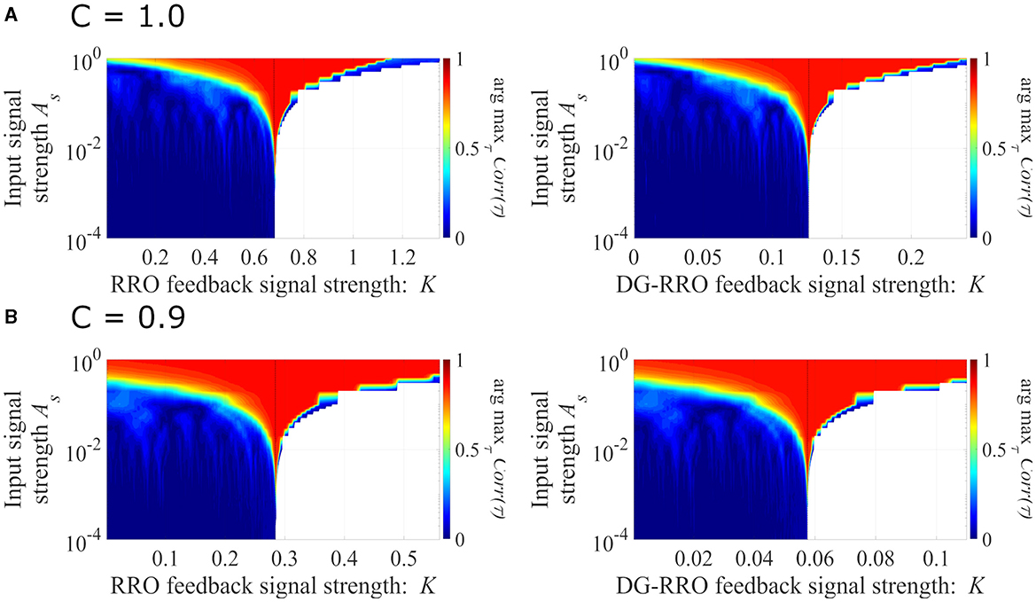
Figure 7. The correlation coefficient arg max_τCorr(τ) between the periodic input signal S(n) and binarised of x(n) according to the feedback strength K and input signal strength. (A) When C = 1.0 and (B) C = 0.9 in noise-free conditions (D_a = 0, D_c = 0) (frequency Ω = 0.005 is set). The black dashed line indicates the attractor-merging bifurcation. In the colored region, CCI occurs; while in the white region, x(n) behavior indicates the absence of CCI. Around the value K for the attractor-merging bifurcation, the synchronization of CCI can be achieved even in smaller signal strength A_s, i.e., the sensitivity of chaotic resonance becomes higher than that at the other regions of K.

Figure 8

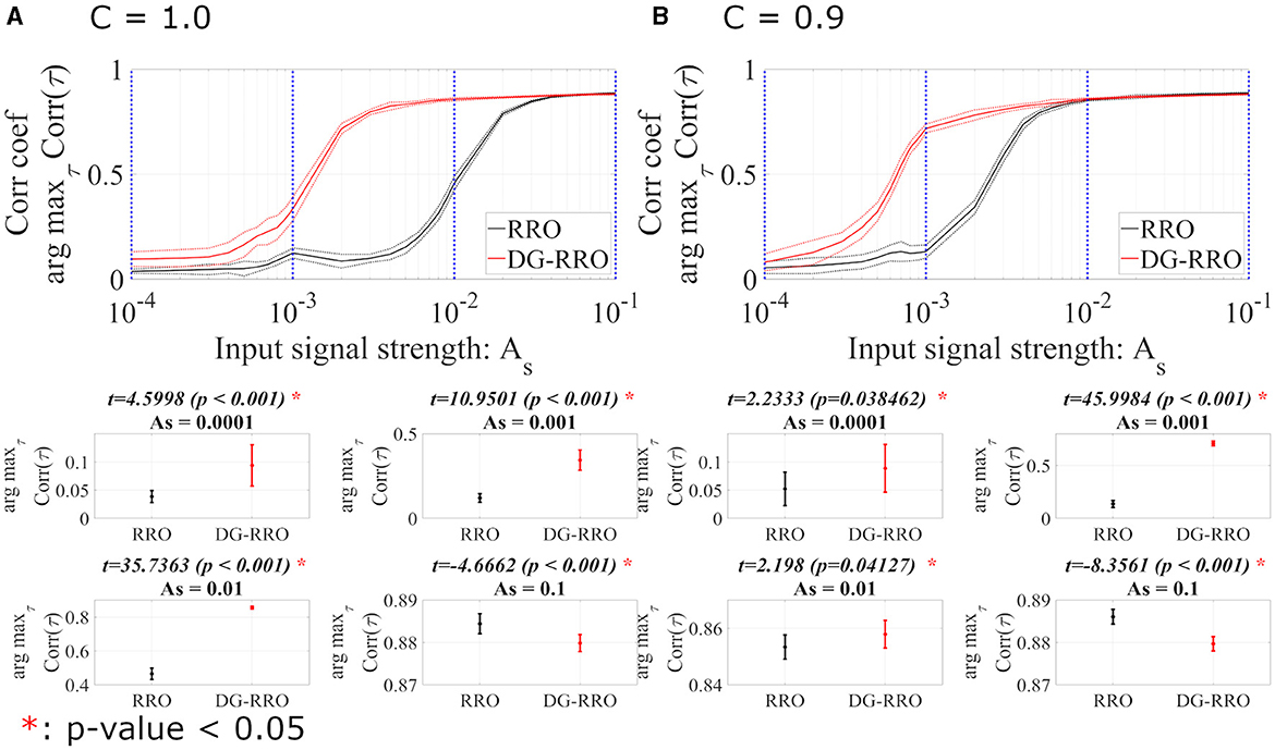
Figure 8. The correlation coefficient arg max_τCorr(τ) between periodic input signal S(n) and binarised x(n) of the DG-RRO method in comparison with the RRO method according to the periodic input strength A_s at the attractor-merging bifurcation. (A) When C = 1.0 and (B) C = 0.9 in noise-free conditions (D_a = 0, D_c = 0). The solid and dashed lines indicate the mean and standard deviation of arg max_τCorr(τ) among 10 trials with Ω = 0.005, respectively. The correlation coefficient arg max_τCorr(τ), when applying the DG-RRO method, exhibited superiority over the RRO method in the input signal strength $10^{-4}\le A_s\le 5\times 10^{-2}$ when C = 1.0 and $10^{-4}\le A_s\le \times 10^{-2}$ when C = 0.9. Some specific values of A_s (corresponding to blue dotted lines) have been chosen to quantify whether the DG-RRO method is superior to the RRO method (t − values > 0) and marked with red asterisks if the statistical criteria of (t-test) (p-values of <0.05).

To investigate the frequency Ω dependence in noise-free conditions (D_a = 0, D_c = 0), Figure 9 shows arg max_τCorr(τ) of both C = 1.0 and C = 0.9 cases at the attractor-merging bifurcation (strength of sinusoidal input signal A_s = 0.01 is set). In the frequency range 10⁻³ ≤ Ω ≤ 10⁻¹, both methods show that when the frequency Ω increases, the arg max_τCorr(τ) decreases. Although arg max_τCorr(τ) decreases, the DG-RRO method maintains a high correlation (arg max_τCorr(τ)>0.7) in the frequency range 10⁻³≲Ω≲9 × 10⁻³ when C = 1.0 and 10⁻³≲Ω≲8 × 10⁻³ when C = 0.9, while the high correlation of the RRO method is maintained in the frequency range 10⁻³≲Ω≲2 × 10⁻³ and 10⁻³≲Ω≲7 × 10⁻³ in both cases.

Figure 9

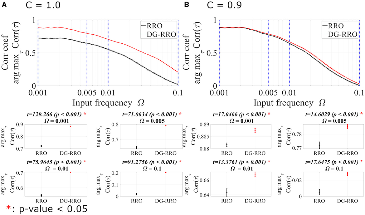
Figure 9. The correlation coefficient arg max_τCorr(τ) between periodic input signal S(n) and binarised of x(n) of the DG-RRO method in comparison with the RRO method according to the input frequency Ω at the attractor-merging bifurcation. (A) When C = 1.0 and (B) C = 0.9 in noise-free conditions (D_a = 0, D_c = 0). The solid and dashed lines indicate the mean and standard deviation of arg max_τCorr(τ) among 10 trials with A_s = 0.01, respectively. The correlation coefficient arg max_τCorr(τ), when applying the DG-RRO method, exhibited superiority over the RRO method in the input frequency range 10⁻⁴ ≤ Ω ≤ 10⁻¹ in both the cases. Some specific values of Ω (corresponding to blue dotted lines) have been chosen to quantify whether the DG-RRO method is superior to the RRO method (t − values > 0) and marked with red asterisks if the statistical criteria of t − test p − values < 0.05. The t − values are almost the same as shown in the bottom part t − values = 17.0466 for Ω = 0.001 and t − values = 17.6475 for Ω = 0.1, i.e., the standard deviation of the correlation for Ω = 0.1 becomes larger even though the difference in the mean value of correlation becomes larger.

3.3 Signal response in the presence of noises

This section reports the investigation results of the effects of noise under chaotic resonance against the RRO and DG-RRO methods. We compared the sensitivity between those methods according to the additive ($10^{-4}\le D_a\le 10^{-1},D_c=0$) and contaminant ($D_a=0,10^{-4}\le D_c\le 10^{-1}$) noise strength at the attractor-merging bifurcation with the determined external input signal (A_s = 0.01, Ω = 0.005). Figures 10, 11 illustrate the arg max_τCorr(τ) of the RRO and DG-RRO methods in the presence of additive and contaminant noise, respectively. Within the additive noise strength $10^{-4}\le D_a\le 10^{-1}$, the arg max_τCorr(τ) of the DG-RRO method is higher than that for the RRO method in the additive noise strength range $10^{-4}\lesssim D_a\lesssim 9\times 10^{-2}$ when C = 1.0 and $10^{-4}\lesssim D_a\lesssim 6\times 10^{-2}$ when C = 0.9. Furthermore, in both cases, the arg max_τCorr(τ) showed a monotonically decreased tendency. However, in this additive noise strength range, the high correlation (arg max_τCorr(τ)>0.7) of the DG-RRO method was sustained in the wider additive noise strength range $10^{-4}\lesssim D_a\lesssim 2.5\times 10^{-3}$ in both cases, while the range with the high correlation of the RRO method was sustained for $10^{-4}\lesssim D_a\lesssim 9\times 10^{-4}$ when C = 1.0 and when $10^{-4}\lesssim D_a\lesssim 2\times 10^{-3}$ when C = 0.9. Furthermore, we investigated the contaminant noise dependency of the RRO and DG-RRO methods (Figure 11). Within the contaminant noise strength range $10^{-4}\le D_c\le 10^{-1}$, as well as additive noise cases, the arg max_τCorr(τ) showed a monotonically decreased tendency in both cases, but the DG-RRO method maintained a higher correlation than the RRO method for the whole range of D_c. Moreover, the high correlation (arg max_τCorr(τ)>0.7) of the DG-RRO method was sustained in the wider contaminant noise strength range $10^{-4}\lesssim D_c\lesssim 4\times 10^{-2}$ when C = 1.0 and $10^{-4}\lesssim D_c\lesssim 7\times 10^{-2}$ when C = 0.9, while with the range with the high correlation of the RRO method which was sustained in the contaminant noise strength range $10^{-4}\lesssim D_c\lesssim 10^{-3}$ when C = 1.0 and $10^{-4}\lesssim D_c\lesssim 3\times 10^{-2}$ when C = 0.9. In summary, compared to the conventional RRO method, the DG-RRO method can sustain high correlation (arg max_τCorr(τ)>0.7) in a wider range of noise and maintain a higher correlation in a certain range.

Figure 10

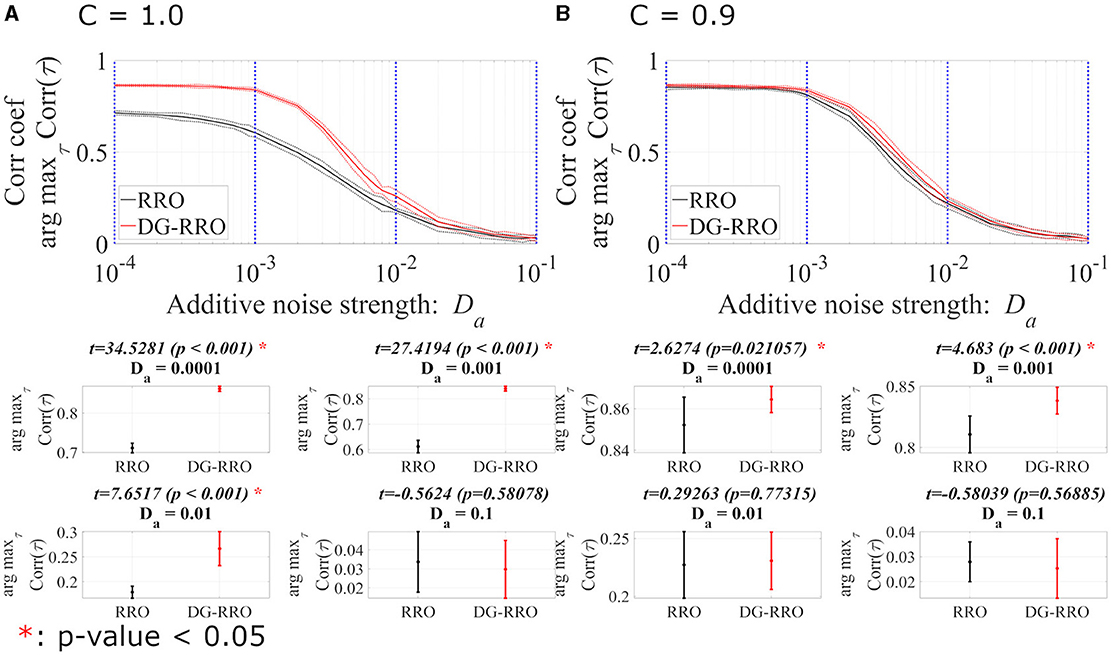
Figure 10. The correlation coefficient arg max_τCorr(τ) between periodic input signal S(n) and binarised x(n) of the DG-RRO method in comparison with the RRO method according to additive noise strength D_a at the attractor-merging bifurcation. (A) When C = 1.0 and (B) C = 0.9. The solid and dashed lines indicate the mean and standard deviation of arg max_τCorr(τ) among 10 trials (A_s = 0.01, Ω = 0.005), respectively. When the DG-RRO method was applied, the feedback signal exhibited a superior correlation coefficient arg max_τCorr(τ) compared with the RRO feedback signal for $D_a\lesssim 9\times 10^{-2}$ when C = 1.0 and for $D_a\lesssim 6\times 10^{-2}$ when C = 0.9. Some specific values of D_a (corresponding to the blue dotted lines) have been chosen to quantify whether the DG-RRO method is superior to the RRO method (t − values > 0) and marked with red asterisks if the statistical criteria of t − test p − values < 0.05.

Figure 11

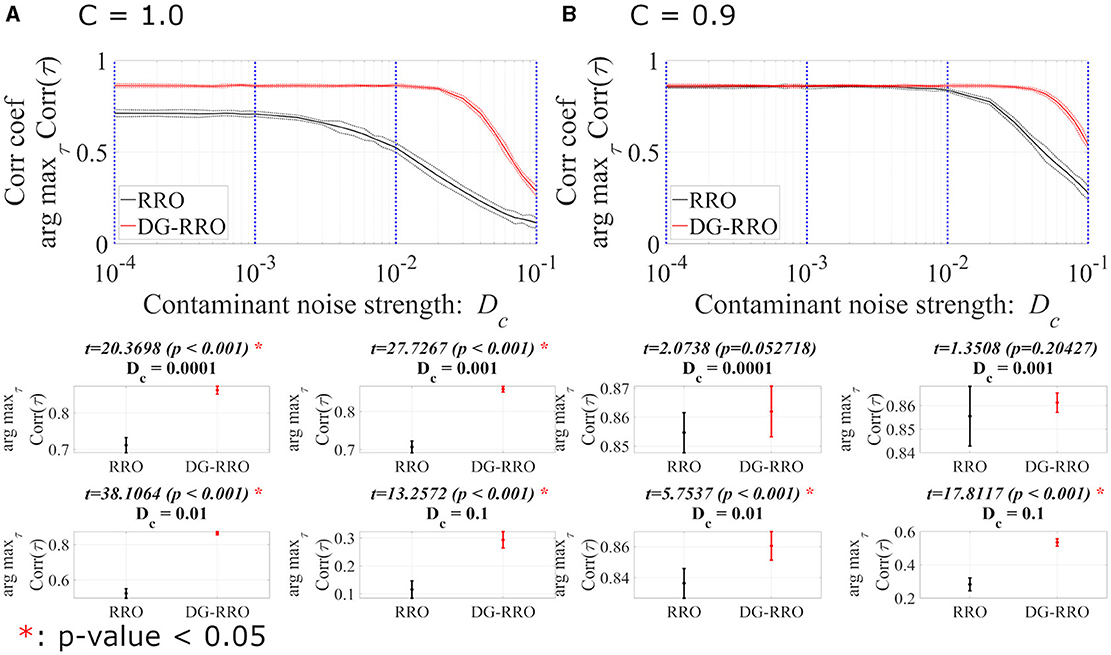
Figure 11. Correlation coefficient arg max_τCorr(τ) between periodic input signal S(n) and binarised of x(n) of the DG-RRO method in comparison with the RRO method according to contaminant noise strength D_c at the attractor-merging bifurcation. (A) When C = 1.0 and (B) C = 0.9. The solid and dashed lines indicate the mean and standard deviation of arg max_τCorr(τ) among 10 trials (A_s = 0.01, Ω = 0.005), respectively. When the DG-RRO method was applied, the feedback signal exhibited a superior correlation coefficient arg max_τCorr(τ) compared with the RRO feedback signal when $10^{-4}\le D_c\le 10^{-1}$ in both cases. Some specific values of D_c (corresponding to the blue dotted lines) have been chosen to quantify whether the DG-RRO method is superior to the RRO method (t − values > 0) and marked with red asterisks if the statistical criteria of t − test p − values of < 0.05.

4 Discussion

In this study, we compared the DG-RRO and the conventional RRO feedback signal to induce CCI synchronization in a mathematical neural system model which includes excitatory and inhibitory neuron populations in the frontal and sensory cortices as typical neural systems with CCI behavior. The DG-RRO feedback method shifts neural activities toward periodic behavior through chaotic resonance. Moreover, this method has higher sensitivity than the conventional RRO method, especially at the attractor-merging bifurcation. Furthermore, under specific ranges of input frequency and strength of additive or contaminant noise, the DG-RRO method sustained a high correlation (arg max_τCorr(τ)>0.7) in a broader range than the RRO method. Moreover, we determined the range of input frequency and strength of noise where $arg{max}_{\tau }\mathrm{\text{Corr}}(\tau )$ of the DG-RRO method is superior to that of the conventional RRO method. Our results demonstrate the potential of the DG-RRO method when applied to neural systems, showing that the DG-RRO method maintained its advantage even in the presence of noise in comparison with the conventional RRO method.

First, we investigated the underlying reason behind the significantly small perturbation Θ caused by the DG-RRO method to achieve attractor-merging bifurcation compared with the conventional RRO method. In the conventional RRO method, the feedback signal has a wide response range of x. However, in the DG-RRO method, by applying double Gaussian functions at approximately local extreme (x_min and x_max), the DG-RRO feedback signal achieved higher local specification around local extreme of the map function (see Figure 5) [36]. Therefore, the feedback signals of the DG-RRO method are considerably smaller than those of the conventional RRO method, except around the local extremes. Accordingly, the amount of perturbation through the time evolution of the DG-RRO feedback signal is much smaller than that of the conventional RRO feedback signal.

Second, we consider the advantages of the DG-RRO method, which has higher sensitivity compared with the RRO method, especially at the attractor-merging bifurcation points. The DG-RRO method can generate CCI with a much smaller perturbation of the feedback signal compared with that of the conventional RRO, as shown in Figure 12, for the DG-RRO feedback signal Kg(x) and the RRO feedback signal Ku(x) at around attractor-merging bifurcation. In the presence of noises, the CCI frequency increases and synchronization is diminished [37, 42]. With such a weaker feedback signal, noise influence might increase. However, the DG-RRO method exhibited the same level of synchronization in comparison with the RRO method. To investigate the causes, Figure 13 illustrates the difference between the conventional RRO and DG-RRO feedback signals. The difference between the range of local minimum (x_min) and maximum (x_max) points for map function F(x) is relatively small in comparison with the other regions. That is, the stronger local specification of the DG-RRO method contributed to maintaining the component of the signal to control attractor-merging bifurcation. By this mechanism, the sensitivity of the DG-RRO feedback signal is still maintained robustness as the RRO feedback signal in the presence of noise. Consequently, the sensitivity of the DG-RRO method is superior to that of the conventional RRO method within a specific range of input frequencies or in the presence of noise of particular strength.

Figure 12

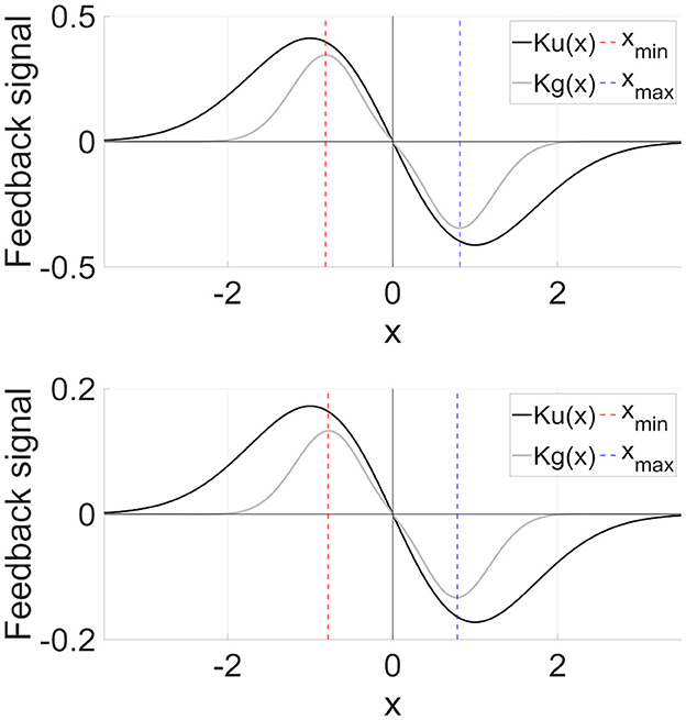
Figure 12. RRO feedback signal Ku(x) and DG-RRO feedback signal Kg(x) in the model with (upper part) C = 1.0, A = 12 and (lower part) C = 0.9, A = 13 which correspond to the attractor bifurcation. The local minimum (x_min)/maximum (x_max) points for map function F(x) given by Equation (2). Feedback signal strength K is fixed in which attractor-merging bifurcation is achieved for each case (upper part) K = 0.6796 for RRO, K = 0.1261 for DG-RRO and (lower part) K = 0.2840 for RRO, K = 0.0575 for DG-RRO. Because the DG-RRO method has higher local specification around local minimum/maximum points than that of the RRO method, the temporal average value of the DG-RRO feedback signal Kg(x) is smaller than those of the RRO feedback signal Ku(x).

Figure 13

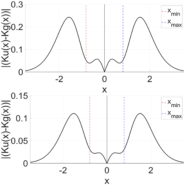
Figure 13. Difference between RRO feedback signal Ku(x) and DG-RRO feedback signal Kg(x) in the model with (upper part) C = 1.0, A = 12 and (lower part) C = 0.9, A = 13 corresponding to the parameters set in Figure 12. Feedback signal strength K is fixed in which attractor-merging bifurcation is achieved for each case (upper part) K = 0.6796 for RRO, K = 0.1261 for DG-RRO and (lower part) K = 0.2840 for RRO, K = 0.0575 for DG-RRO.

The limitations of this study must be considered. This study used a simple mathematics neural model system, including frontal and sensory cortices, to reproduce neural activity. However, real neural activity exhibits more complicated dynamic characteristics. Implementing such strategies in practice presents numerous challenges from a technical standpoint. Directly applying external signals to specific regions of the human brain, particularly the frontal cortex, involves intricate procedures. Therefore, the effectiveness of the DG-RRO method in more physiologically realistic neural systems should be validated in future studies. In previous studies, it has been reported that the RRO method can transit neural activity to a periodic state with a circadian period in a mathematics model, which reproduced the neural activities of patients with BD by managing the light stimulus of the chronotherapy method [18, 34]. Based on the result of this study, the DG-RRO method can reduce the intervention to the mathematics model of neural network to extremely low levels because the amount of required perturbation is weaker than that of the conventional RRO method. Despite many validations and considerable conditions before applying to practical neural networks, this property of the DG-RRO method can be considered in reducing the side effects of over-intervention, such as light therapy treatment for hyperactivity or hypomania [18, 34]. This point must be studied in future studies.

In conclusion, this study illustrates the capability of the DG-RRO method to effectively control chaotic resonance with extremely weak feedback signals in the mathematics excitatory–inhibitory neural systems exhibiting CCI behavior. Our findings confirm that the DG-RRO method induces minor perturbations while maintaining higher sensitivity compared with the conventional RRO method. Notably, the heightened sensitivity of the DG-RRO method persists even in the presence of noise within a specific range. Despite the inherent limitations of our model-based approach, these results underscore the potential application of the DG-RRO approach in neural systems. Further research for validation with more practical models of this methodology offers new avenues for addressing complex neurological disorders.

Data availability statement

The raw data supporting the conclusions of this article will be made available by the authors, without undue reservation.

Author contributions

AT: Writing – original draft, Writing – review & editing. SN: Writing – original draft, Writing – review & editing. NW: Writing – review & editing. KI: Writing – review & editing. HD: Writing – review & editing. TY: Writing – review & editing. HN: Writing – review & editing.

Funding

The author(s) declare financial support was received for the research, authorship, and/or publication of this article. This study was supported by JSPS KAKENHI for Scientific Research (C) [(grant number: JP22K12183) (SN), (grant number: JP22K12194) (HD), (grant number: JP22K02926) (TY), and (grant number: JP20K11976) (HN)] and JSPS KAKENHI Grant-in-Aid for Transformative Research Areas (A) (Grant Number JP20H05921) (SN).

Conflict of interest

The authors declare that the research was conducted in the absence of any commercial or financial relationships that could be construed as a potential conflict of interest.

Publisher's note

All claims expressed in this article are solely those of the authors and do not necessarily represent those of their affiliated organizations, or those of the publisher, the editors and the reviewers. Any product that may be evaluated in this article, or claim that may be made by its manufacturer, is not guaranteed or endorsed by the publisher.

References

1. Tadokoro Y, Tanaka H, Nakashima Y, Yamazato T, Arai S. Enhancing a BPSK receiver by employing a practical parallel network with stochastic resonance. Nonlinear theory and its applications. IEICE. (2019) 10:106–14. doi: 10.1587/nolta.10.106

PubMed Abstract | Crossref Full Text | Google Scholar

2. Ibáñez S, Fierens P, Perazzo R, Patterson G, Grosz D. On the dynamics of a single-bit stochastic-resonance memory device. Eur Phys J. (2010) 76:49–55. doi: 10.1140/epjb/e2010-00180-8

Crossref Full Text | Google Scholar

3. Stotland A, Di Ventra M. Stochastic memory: memory enhancement due to noise. Physical Review E. (2012) 85:011116. doi: 10.1103/PhysRevE.85.011116

PubMed Abstract | Crossref Full Text | Google Scholar

4. Enders LR, Hur P, Johnson MJ, Seo NJ. Remote vibrotactile noise improves light touch sensation in stroke survivors fingertips via stochastic resonance. J Neuroeng Rehabil. (2013) 10:105. doi: 10.1186/1743-0003-10-105

PubMed Abstract | Crossref Full Text | Google Scholar

5. Kurita Y, Shinohara M, Ueda J. Wearable sensorimotor enhancer for fingertip based on stochastic resonance effect. IEEE Trans Human-Mach Syst. (2013) 43:333–7. doi: 10.1109/TSMC.2013.2242886

Crossref Full Text | Google Scholar

6. Kurita Y, Sueda Y, Ishikawa T, Hattori M, Sawada H, Egi H, et al. Surgical grasping forceps with enhanced sensorimotor capability via the stochastic resonance effect. IEEE/ASME Trans Mechatron. (2016) 21:2624–34. doi: 10.1109/TMECH.2016.2591591

Crossref Full Text | Google Scholar

7. Van der Groen O, Tang MF, Wenderoth N, Mattingley JB. Stochastic resonance enhances the rate of evidence accumulation during combined brain stimulation and perceptual decision-making. PLoS Comput Biol. (2018) 14:e1006301. doi: 10.1371/journal.pcbi.1006301

PubMed Abstract | Crossref Full Text | Google Scholar

8. Guo D, Perc M, Liu T, Yao D. Functional importance of noise in neuronal information processing. Europhys Lett. (2018) 124:50001. doi: 10.1209/0295-5075/124/50001

Crossref Full Text | Google Scholar

9. Palabas T, Torres JJ, Perc M, Uzuntarla M. Double stochastic resonance in neuronal dynamics due to astrocytes. Chaos, Solitons Fractals. (2023) 168:113140. doi: 10.1016/j.chaos.2023.113140

PubMed Abstract | Crossref Full Text | Google Scholar

10. Harmer GP, Davis BR, Abbott D. A review of stochastic resonance: circuits and measurement. IEEE Trans Instrum Meas. (2002) 51:299–309. doi: 10.1109/19.997828

Crossref Full Text | Google Scholar

11. Rosenblum M, Pikovsky A. Synchronization: from pendulum clocks to chaotic lasers and chemical oscillators. Contemp Phys. (2003) 44:401–16. doi: 10.1080/00107510310001603129

Crossref Full Text | Google Scholar

12. Baysal V, Yilmaz E. Chaotic signal induced delay decay in Hodgkin-Huxley Neuron. Appl Mathemat Comp. (2021) 411:126540. doi: 10.1016/j.amc.2021.126540

Crossref Full Text | Google Scholar

13. Anishchenko VS, Astakhov V, Neiman A, Vadivasova T, Schimansky-Geier L. Nonlinear Dynamics of Chaotic and Stochastic Systems: Tutorial and Modern Developments. Cham: Springer Science & Business Media. (2007).

Google Scholar

14. Rajasekar S, Sanjuán MAF. Nonlinear Resonances. Cham: Springer (2016). doi: 10.1007/978-3-319-24886-8

Crossref Full Text | Google Scholar

15. Nobukawa S, Nishimura H. Synchronization of chaos in neural systems. Front Appl Mathemat Statist. (2020) 6:19. doi: 10.3389/fams.2020.00019

Crossref Full Text | Google Scholar

16. Nishimura H, Katada N, Aihara K. Coherent response in a chaotic neural network. Neural Proc Lett. (2000) 12:49–58. doi: 10.1023/A:1009626028831

PubMed Abstract | Crossref Full Text | Google Scholar

17. Nobukawa S, Nishimura H, Yamanishi T. Evaluation of chaotic resonance by Lyapunov exponent in attractor-merging type systems. In: International Conference on Neural Information Processing. Cham: Springer (2016). p. 430–437.

Google Scholar

18. Nobukawa S, Nishimura H, Wagatsuma N, Inagaki K, Yamanishi T, Takahashi T. Recent trends of controlling chaotic resonance and future perspectives. Front Appl Mathemat Statist. (2021) 7:760568. doi: 10.3389/fams.2021.760568

Crossref Full Text | Google Scholar

19. Schweighofer N, Doya K, Fukai H, Chiron JV, Furukawa T, Kawato M. Chaos may enhance information transmission in the inferior olive. Proc Nat Acad Sci. (2004) 101:4655–60. doi: 10.1073/pnas.0305966101

PubMed Abstract | Crossref Full Text | Google Scholar

20. Tokuda IT, Han CE, Aihara K, Kawato M, Schweighofer N. The role of chaotic resonance in cerebellar learning. Neural Networks. (2010) 23:836–42. doi: 10.1016/j.neunet.2010.04.006

PubMed Abstract | Crossref Full Text | Google Scholar

21. Nobukawa S, Nishimura H, Yamanishi T, Liu JQ. Analysis of chaotic resonance in Izhikevich neuron model. PLoS ONE. (2015) 10:e0138919. doi: 10.1371/journal.pone.0138919

PubMed Abstract | Crossref Full Text | Google Scholar

22. Nobukawa S, Nishimura H. Chaotic resonance in coupled inferior olive neurons with the Llinás approach neuron model. Neural Comput. (2016) 28:2505–32. doi: 10.1162/NECO_a_00894

PubMed Abstract | Crossref Full Text | Google Scholar

23. Nobukawa S, Nishimura H, Yamanishi T. Chaotic resonance in typical routes to chaos in the Izhikevich neuron model. Sci Rep. (2017) 7:1–9. doi: 10.1038/s41598-017-01511-y

PubMed Abstract | Crossref Full Text | Google Scholar

24. Baysal V, Erkan E, Yilmaz E. Impacts of autapse on chaotic resonance in single neurons and small-world neuronal networks. Philos Trans R Soc A. (2021) 379:20200237. doi: 10.1098/rsta.2020.0237

PubMed Abstract | Crossref Full Text | Google Scholar

25. Nobukawa S, Doho H, Shibata N, Nishimura H, Yamanishi T. Chaos-chaos intermittency synchronization controlled by external feedback signals in Chua's circuits. IEICE Trans Fundam Electron Comput Sci. (2020) 103:303–12. doi: 10.1587/transfun.2019EAP1081

PubMed Abstract | Crossref Full Text | Google Scholar

26. Anishchenko VS, Safonova M, Chua LO. Stochastic resonance in the nonautonomous Chua's circuit. J Circu. Syst. Comp. (1993) 3:553–78. doi: 10.1142/S0218126693000344

Crossref Full Text | Google Scholar

27. Nobukawa S, Shibata N. Controlling chaotic resonance using external feedback signals in neural systems. Sci Rep. (2019) 9:4990. doi: 10.1038/s41598-019-41535-0

PubMed Abstract | Crossref Full Text | Google Scholar

28. Nobukawa S, Shibata N, Nishimura H, Doho H, Wagatsuma N, Yamanishi T. Resonance phenomena controlled by external feedback signals and additive noise in neural systems. Sci Rep. (2019) 9:1–15. doi: 10.1038/s41598-019-48950-3

PubMed Abstract | Crossref Full Text | Google Scholar

29. Sinha S. Noise-free stochastic resonance in simple chaotic systems. Physica A Stat. (1999) 270:204–14. doi: 10.1016/S0378-4371(99)00136-3

Crossref Full Text | Google Scholar

30. Hadaeghi F, Hashemi Golpayegani MR, Jafari S, Murray G. Toward a complex system understanding of bipolar disorder: a chaotic model of abnormal circadian activity rhythms in euthymic bipolar disorder. Aust N Z J Psychiatry. (2016) 50:783–92. doi: 10.1177/0004867416642022

PubMed Abstract | Crossref Full Text | Google Scholar

31. Baghdadi G, Jafari S, Sprott J, Towhidkhah F, Golpayegani MH. A chaotic model of sustaining attention problem in attention deficit disorder. Commun Nonlinear Sci Numer Simul. (2015) 20:174–85. doi: 10.1016/j.cnsns.2014.05.015

Crossref Full Text | Google Scholar

32. Baysal V, Saracc Z, Yilmaz E. Chaotic resonance in Hodgkin-Huxley neuron. Nonlin Dynam. (2019) 97:1275–85. doi: 10.1007/s11071-019-05047-w

Crossref Full Text | Google Scholar

33. Nobukawa S, Nishimura H, Yamanishi T, Doho H. Controlling chaotic resonance in systems with chaos-chaos intermittency using external feedback. IEICE Trans Fundam Electron Comput Sci. (2018) 101:1900–6. doi: 10.1587/transfun.E101.A.1900

PubMed Abstract | Crossref Full Text | Google Scholar

34. Doho H, Nobukawa S, Nishimura H, Wagatsuma N, Takahashi T. Transition of neural activity from the chaotic bipolar-disorder state to the periodic healthy state using external feedback signals. Front Comput Neurosci. (2020) 14:76. doi: 10.3389/fncom.2020.00076

PubMed Abstract | Crossref Full Text | Google Scholar

35. Nobukawa S, Wagatsuma N, Nishimura H, Doho H, Takahashi T. An Approach for stabilizing abnormal neural activity in ADHD using chaotic resonance. Front Comp Neurosci. (2021) 76:726641. doi: 10.3389/fncom.2021.726641

PubMed Abstract | Crossref Full Text | Google Scholar

36. Iinuma T, Ebato E, Nobukawa S, Tran AT, Wagatsuma N, Inagaki K, et al. Extremely weak feedback method for controlling chaotic resonance. In: 2022 IEEE International Conference on Systems, Man, and Cybernetics (SMC). Honolulu : IEEE (2022). doi: 10.1109/SMC53992.2023.10394470

Crossref Full Text | Google Scholar

37. Nobukawa S, Wagatsuma N, Nishimura H, Inagaki K, Yamanishi T. Influence of additive and contaminant noise on control-feedback induced chaotic resonance in excitatory-inhibitory neural systems. IEICE Trans Fundam Electron Comput Sci. (2023) 106:11–22. doi: 10.1587/transfun.2022EAP1024

PubMed Abstract | Crossref Full Text | Google Scholar

38. Pikovsky A, Rosenblum M, Kurths J. Synchronization: A Universal Concept in Nonlinear Sciences. Cambridge: Cambridge University Press. (2003).

Google Scholar

39. Mazaheri A, Coffey-Corina S, Mangun GR, Bekker EM, Berry AS, Corbett BA. Functional disconnection of frontal cortex and visual cortex in attention-deficit/hyperactivity disorder. Biol Psychiatry. (2010) 67:617–23. doi: 10.1016/j.biopsych.2009.11.022

PubMed Abstract | Crossref Full Text | Google Scholar

40. Moriyama TS, Polanczyk G, Caye A, Banaschewski T, Brandeis D, Rohde LA. Evidence-based information on the clinical use of neurofeedback for ADHD. Neurotherapeutics. (2012) 9:588–98. doi: 10.1007/s13311-012-0136-7

PubMed Abstract | Crossref Full Text | Google Scholar

41. Bayani A, Hadaeghi F, Jafari S, Murray G. Critical slowing down as an early warning of transitions in episodes of bipolar disorder: a simulation study based on a computational model of circadian activity rhythms. Chronobiol Int. (2017) 34:235–45. doi: 10.1080/07420528.2016.1272608

PubMed Abstract | Crossref Full Text | Google Scholar

42. Nobukawa S, Wagatsuma N, Nishimura H, Doho H, Takahashi T. An approach for stabilizing abnormal neural activity in ADHD using chaotic resonance. Front Comp Neurosci. (2021) 76:726641. doi: 10.3389/fncom.2021.726641

PubMed Abstract | Crossref Full Text | Google Scholar