Dynamic study of the duopoly market stability based on open innovation rate integration and intellectual property

In this paper, we present a model detailing the benefits of two competing firms in a duopoly market, where profit maximization is linked to their production levels using the Cournot method. Our primary objective is to develop a collaborative strategy within the framework of open innovation to optimize their profits. Furthermore, we analyze how these firms can integrate an additional source of revenue in the form of intellectual property, without negatively impacting their open innovation strategies. To achieve this, we conducted a dynamic study of these strategies by introducing this intellectual property, to assess the impact of its components, such as patent licensing fees and royalties, on the equilibrium of strategies adopted by these firms. Our aim is to provide recommendations for optimal management of this intellectual property, thus enabling firms to fully leverage its benefits while preserving their competitive position in the market.

1 Introduction

Researchers from around the world have studied and defined Open Innovation as an important concept in innovation management. Over the past two decades, this phenomenon has become a principle for many organizations in various industry sectors. Recent opportunities for adopting and creating value through Open Innovation during periods of global crisis, such as the pandemic, are demonstrated through concrete examples (1–5).

Furthermore, the role of startups and entrepreneurial spirit is illustrated through examples from the life sciences industry (6). Intellectual property, which includes patents and rights over non-patented intellectual property, as well as the right to sublicense IP, product development and manufacturing rights, and marketing rights, constitutes elements of value capture rights in innovation. Ozmel et al. (7) were the first to introduce the term “value capture rights.”

An intellectual property strategy is characterized as “the utilization of intellectual property, whether independently or in conjunction with other assets of the company, to accomplish the company’s strategic goals (8).

The complex relationship between Open Innovation (OI) and Intellectual Property (IP) protection has been the subject of numerous research studies, revealing clear evidence of their connection. Due to this intricate relationship, several authors have delved into this topic in their research papers (9–12). They have focused on the impact of IP on OI. A study based on 73 companies examines the correlation between intellectual property protection strategies and open innovation, identifying five distinct strategies and evaluating their impact on open innovation practices. The findings underscore the critical role of strategic choices regarding intellectual property in promoting and managing innovation within organizations (10). Moreover, the need for intellectual property is a strong driver of open innovation. These arguments are verified using firm-level data from Vietnam, and supporting evidence is obtained, demonstrating that, contrary to conventional wisdom, the need for intellectual property protection encourages companies to engage in open innovation activities (12). In another study focusing on Italian companies, a framework is proposed for using intellectual property (IP) protection mechanisms to secure technology and know-how during the innovation process. This research highlights increased efficiency, emphasizing the importance of managerial and organizational interventions. Additionally, it analyzes how these mechanisms can act as facilitators, catalysts, or constraints for innovation collaborations (9).

Compared to closed innovation, intellectual property (IP) protection created within the framework of open innovation is complex. A robust IP management policy focused on reducing IP risks plays a significant role in ensuring sustained growth. These risks vary across business segments, from startups to micro, small, medium, and large organizations. A risk assessment model for intellectual property in open innovation is proposed by Arunnima et al. (13) to calculate the Open Innovation Intellectual Property Risk Score (OIIPRS) using an Analytical Hierarchy Process (AHP) method. The OIIPRS indicates an organization’s levels of IP risk when engaging in open innovation with other organizations. Companies can use the OIIPRMM to assess IP risk levels and adopt proactive IP protection mechanisms when collaborating with other organizations (13).

To the best of our knowledge, studies of IP strategies and OI are scarce, and none of them organically presented how different IP strategies shape firms’ capability to leverage and benefit from OI. Such a gap is critical since much of the current literature could lead practitioners to think that a certain mix of IPPMs may be better than another, whereas the very same mix, used with different IP strategies, may achieve dramatically different outcomes.

Grimaldi et al. propose a framework comprising three intellectual property (IP) protection strategies: the “defensive” strategy, which aims to prevent knowledge leakage and erect barriers to competition; the “collaborative” strategy, which aims to collaborate with other organizations and penetrate new markets; and an “impromptu “strategy, which describes firms protecting their IP without a predetermined objective (11). According to the findings, most firms declare adopting an impromptu IP strategy. Such a strategy can impede outbound open innovation (OI), while firms adopting a defensive IP strategy are more active in outbound OI than those adopting a collaborative IP strategy. Finally, the results show that firms adopting collaborative IP strategies outperform those adopting defensive strategies (11, 14, 15).

Game theory has proven to be a useful tool for modeling the interactions that take place in Open Innovation ecosystems. More specifically, the Cournot duopoly has emerged as a popular game theory model for simulating the strategic behavior of firms in the context of Open Innovation.

Game theory, as a framework for analyzing strategic interactions, is an essential tool for studying Open Innovation (OI) and its relationship with intellectual property (IP) (16). explore how competition and intellectual property protection influence dynamics in a duopoly involving both foreign and domestic enterprises. Their research aims to understand stability near equilibrium points and how different scenarios affect R&D investment dynamics, considering cases where one or both enterprises are engaged in R&D activities. Moreover, Ikeda et al. (17) investigate the ideal intellectual property rights policies for a large market country without local producers. They find that prohibiting imitation, especially with low innovation costs, can enhance societal welfare, even in a monopoly environment.

Additionally, Zhang et al. (18) propose a model based on game theory to analyze how firms choose between innovation and imitation, considering behavioral biases like reference point dependence and loss aversion. Their study highlights the importance of managing innovation risks and the effectiveness of strengthening IP protection in influencing firms’ innovation strategies. Meanwhile, Xing (19) delves into the dynamics of competition between open-source software (OSS) and proprietary software (PS) in a networked software market. Using a modified Cournot model, Xing explores how OSS learning costs, user software development skills, and network effects impact the optimal pricing, quantity, and profitability strategies of both PS and OSS. Lastly, Bao et al. (20) demonstrate that cooperative game strategies can lead to a more equitable distribution of excess earnings produced from cooperation innovation, based on Rubinstein subgame perfect equilibrium results.

This article seems to address an interesting analysis of competitive dynamics in the market, based on the Cournot model to evaluate the quantities of products present on the market. However, it is important to note that a discussion of intellectual property (IP) is missing, which could potentially have a significant impact on the study results. IP is a crucial aspect in many industries, especially when it comes to open innovation. Without a discussion of how IP is treated in the model, it is difficult to fully assess the validity of the results and their applicability in a real-world context. For example, the way intellectual property rights are defined and protected can have a major impact on the open innovation strategy adopted by companies, as well as on competitive dynamics in the market. With this in mind, further study should take into account how IP is integrated into the analysis model. This could involve examining how companies manage intellectual property rights as part of their open innovation strategy, how these rights influence product quantity decisions in the market, and how they affect the competitive outcomes achieved.

The recent work of Elmire et al. (21) examines an analysis of OI in a duopolistic market using game theory, however, the intellectual property parameter is not taken into account to study the stability of the firm in the duopolistic market.

In this work, a dynamic study of the impact of IP parameters on the stability of the duopoly market is presented. The studied dynamic system is based on the OI integration rate of the both firms. The remaining of this work is as following: the second section is dedicated to present the proposed model based on the IP and OI interaction. The third section presents the dynamic adjustment process of the two firms. The fourth section concerns the study of the stability of all the computed equilibrium points, and finally, the principal finding based on the analysis of bifurcation diagrams and stability map are present in the fifth section.

2 Cournot duopoly model

Gaining a comprehensive understanding of open innovation systems and investigating the effects of varying market structures, open innovation investment levels, and intellectual property rights on business performance and market outcomes are the goals.

The model is built upon the presence of two firms, denoted as i (i = 1,2), operating in a market where identical products are offered. The inverse demand function for these two firms is derived from the maximization of a utility function, which can be expressed as:

$\begin{array}{ll}{p}_i=a-b\left(q_1+q_2\right)& (1)\end{array}$

where, $a>0$and $b\in \left[0,1\right]\text{,}$ $q_1$and $q_2$ are the output of the products quantity provided by the firm 1 and firm 2, respectively.

In this work, we have considered that both firms are making strategic decisions regarding the incorporation of innovation into their operations. To model the adoption of Open Innovation (OI) strategies, we introduce the parameter ${\sigma }_i\in \left[0,1\right]$ . This parameter serves as a crucial factor representing the OI integration rate, allowing us to quantify the extent to which each firm embraces Open Innovation practices within the range from 0 (completely closed innovation) to 1 (fully open innovation).

According these assumptions, the effective marginal cost of firm i can be expressed as

$\begin{array}{ll}{C}_i\left({\sigma }_i\right)=A+c\left(1-{\sigma }_i\right),i=1,2& (2)\end{array}$

The cost function values are contingent on the OI integration rate. When a firm i opts to outsource its innovation, the marginal cost remains at $A$ , as the integration rate ${\sigma }_i$equals one. Conversely, if firm i chooses to completely internalize the innovation, the marginal cost increases to $A+c$ , reflecting the additional cost incurred due to the internalization of the innovation process.

Considering the advantages associated with Closed Innovation (CI), such as robust incentives, firm-owned property rights, and decreased reuse costs, it becomes apparent that as a firm elevates its Open Innovation rate, it relinquishes these benefits. Consequently, this represents a loss incurred by the firm due to the extensive utilization of Open Innovation. These foregone benefits can be viewed as costs or charges imposed on the firm, adding to its overall cost structure and reducing its competitive advantage.

We assume that the two firms practice the OI concept with a rate ${\sigma }_i\text{.}$ In addition, one of the firm sells patent to the other firm with a price L_i, in this case, if firm 2 get the patent from firm 1, it should paid the license fees to the firm 1 upon the signing of the agreement, and the royalty that represent a share of the revenues paid to the licensor in exchange for rights. It can be a fixed amount, a percentage of the revenues, or an amount per unit sold, and so on. Often, a minimum of royalty is required (22). In this work, the royalty is represented by $\alpha q_i$ . Consequently, the firm 2 should paid $L_1+\alpha q_2$ (The assumption is always Firm 1 is the seller of the patent, and Firm 2 is the buyer of the patent).

According to Chesbrough, the PI protection is related to the innovation strategy, especially, the firms that adopt CI protect more its PI (23). Considering firm 1 adopts CI, in this case, it is possible that this firm sells the patent to firm 2 with a fee of $L_2$ , for this reason we consider two patents fees $L_1$ and $L_2$ and the same royalty $\alpha$ . In the case of firm 1 sells patent to firm 2, the profit of intellectual property can be expressed as:

$\begin{array}{ll}{\eta }_1=\left(\alpha q_2+L_1\right)\left(1-{\sigma }_1\right)& (3)\end{array}$

The intellectual property profit is important when the firm practice closed innovation ( ${\sigma }_1=0$ ). In other words, they are no IP protection when the firm practice totally OI (23).

Based on the aforementioned proposals, the expression of the profit for both firms is defined as:

$\{\begin{array}{c}\hfill {\pi }_1=\left[p_1\left(q_1,q_2\right)-C_1\left({\sigma }_1,{\sigma }_2\right)\right]q_1+{\eta }_1\left({\sigma }_1,q_2\right)\hfill \\ \hfill {\pi }_2=\left[p_2\left(q_1,q_2\right)-C_2\left({\sigma }_1,{\sigma }_2\right)\right]q_2+{\eta }_2\left({\sigma }_2,q_1\right)\hfill \end{array}\text{ (4)}$

By substituting Equations (1)–(3) into Equation (4), we obtain the expression of the profit function for each firm as:

$\{\begin{array}{c}\hfill {\pi }_1=-b{q}_1^2+\left(a-b{q}_2-A-c\left(1-{\sigma }_1\right)\right)q_1+\left(\alpha q_2+L_1\right)\left(1-{\sigma }_1\right)\hfill \\ \hfill {\pi }_2=-b{q}_2^2+\left(a-b{q}_1-A-c\left(1-{\sigma }_2\right)\right)q_2+\left(\alpha q_1+L_2\right)\left(1-{\sigma }_2\right)\hfill \end{array}\text{ (5)}$

Then, the marginal profits of these two firms are expressed by Equation (6).

$\{\begin{array}{c}\hfill \frac{\partial {\pi }_1}{\partial q_1}=-2b{q}_1+\left(a-b{q}_2-A-c\left(1-{\sigma }_1\right)\right)\hfill \\ \hfill \frac{\partial {\pi }_2}{\partial q_2}=-2b{q}_2+\left(a-b{q}_1-A-c\left(1-{\sigma }_2\right)\right)\hfill \end{array}\text{ (6)}$

The second-order conditions are met because $\frac{{\partial }^2{\pi }_1}{{\partial }^2{q}_1}=\frac{{\partial }^2{\pi }_2}{{\partial }^2{q}_2}=-2b<0$ . Letting $\frac{\partial {\pi }_i}{\partial q_i}=0$ (i = 1,2), the reaction function of the firm 1 and firm 2 is obtained as follow:

$\{\begin{array}{c}\hfill R_1\left(q_2,{\sigma }_1\right)=q_1^{\ast }=\frac{a-b{q}_2-A-c\left(1-{\sigma }_1\right)}{2b}\hfill \\ \hfill R_2\left(q_1,{\sigma }_2\right)=q_2^{\ast }=\frac{a-b{q}_1-A-c\left(1-{\sigma }_2\right)}{2b}\hfill \end{array}\text{ (7)}$

The reaction function in a Cournot model describes how one firm’s output (or quantity) depends on the output chosen by its competitors. From Equation (7), we obtain the equilibrium solution for the two firms as following:

$\{\begin{array}{c}\hfill q_1^{\ast }=U-\frac{c}{3b}\left({\sigma }_2-2{\sigma }_1\right)\hfill \\ \hfill q_2^{\ast }=U-\frac{c}{3b}\left({\sigma }_1-2{\sigma }_2\right)\hfill \end{array}\text{ (8)}$

With $U=\frac{\left(a-A-c\right)}{3b}$ . Also, by subtracting $q_1^{\ast }$ from $q_2^{\ast }$ , we obtain:

$\begin{array}{ll}\mathrm{\Delta }q=q_1^{\ast }-q_2^{\ast }=\frac{c}{b}\left({\sigma }_1-{\sigma }_2\right)& (9)\end{array}$

By analyzing the Δq value (Equation 9), it becomes evident that the equilibrium quantities are contingent upon the innovation integration rates adopted by each firm. Assuming that firm 1 opts for an Open Innovation (OI) approach (σ₁ = 1) and firm 2 selects Closed Innovation (CI) as the opposing strategy (σ₂ = 0), where Δq > 0, it implies that firm 1 consistently produces quantities surpassing those of firm 2. Consequently, a higher OI integration rate results in the firm delivering greater quantities. The Cournot equilibrium can be expressed by substituting $q_1^{\ast }$ and $q_2^{\ast }$ in the reaction function. Substituing Equation 8 in Equation 5, we obtain the system shown by Equation (10). In this system, the two firm’s the equilibrium profits are expressed in terms of the OI integration rate, and we notice that the equilibrium profit is expressed in parabolic function ( ${\sigma }_1^2,{\sigma }_2^2$ ), linear function ( ${\sigma }_1,{\sigma }_2$ ) and an interaction function ( ${\sigma }_1{\sigma }_2)$ .

$\left\{\begin{array}{c}\begin{array}{l}{\pi }_1=\frac{c}{9b}\left(2c+3\alpha \right){\sigma }_1^2-\frac{c^2}{9b}{\sigma }_2^2-\frac{1}{3b}\left(b\left(3\alpha +3L_1-5cU\right)+\alpha \right){\sigma }_1\\ +\frac{c}{3b}\left(2c-bU\right){\sigma }_2+\frac{1}{9b}c\left(c-6\alpha \right){\sigma }_1{\sigma }_2+U\left(\alpha +2bU\right)+L_1\end{array}\\ \begin{array}{l}{\pi }_2=\frac{c}{9b}\left(2c+3\alpha \right){\sigma }_2^2-\frac{c^2}{9b}{\sigma }_1^2-\frac{1}{3b}\left(b\left(3\alpha +3L_2-5cU\right)+\alpha \right){\sigma }_1\\ +\frac{c}{3b}\left(2c-bU\right){\sigma }_2+\frac{1}{9b}c\left(c-6\alpha \right){\sigma }_1{\sigma }_2+U\left(\alpha +2bU\right)+L_2\end{array}\end{array}\right.\left(10\right)$

The relative profits $\mathrm{\Delta }{\pi }_{\text{i}}$ (i = 1,2) of each firm can be expressed as the difference between the absolute profit of itself and the absolute profit of its competitor (24). The relative profit of firm 1 is expressed by Equation (11).

According to Equation (11), the relative profit expressed by Equation (11) depends on the rate of integration of OI, intellectual property, and other economic parameters.

$\begin{array}{c}\mathrm{\Delta }{\pi }_1={\pi }_1-{\pi }_2=\left(\frac{c}{3b}\left(c+\alpha \right)\left({\sigma }_2+{\sigma }_1\right)+\left(\frac{\alpha \left(3\alpha +1\right)}{3b}-\frac{7cU}{6}\right)\right)\\ \left({\sigma }_2-{\sigma }_1\right)+L_1\left({\sigma }_1-1\right)-L_2\left({\sigma }_2-1\right)\end{array}\text{ (11)}$

Therefore, we can identify various scenarios based on the strategies adopted by the two firms.

• Case 1: ${\sigma }_1=0and{\sigma }_2=1$

In this case, the two firms are symmetrical where firm 1 adopts close innovation and firm 2 adopts totally Open innovation. Consequently, the relative profit becomes:

$\begin{array}{ll}\mathrm{\Delta }\pi =\left(\frac{c}{3b}\left(c+\alpha \right)+\left(\frac{\alpha \left(3\alpha +1\right)}{3b}-\frac{7cU}{6}\right)\right)-L_1& (12)\end{array}$

If Firm 1 wants to achieve a profit higher than Firm 2, it must sell its patents at a price $L_1<\left(\frac{c}{3b}\left(c+\alpha \right)+\left(\frac{\alpha \left(3\alpha +1\right)}{3b}-\frac{7cU}{6}\right)\right)$ , and if $L_1>\left(\frac{c}{3b}\left(c+\alpha \right)+\left(\frac{\alpha \left(3\alpha +1\right)}{3b}-\frac{7cU}{6}\right)\right)$ it will realize a profit lower than Firm 2.

• Case 2: ${\sigma }_1={\sigma }_2=\sigma$

In this case, the two firms adopt the same level of openness with ${\sigma }_1={\sigma }_2=\sigma$ ; therefore, the relative profit becomes:

$\begin{array}{ll}\mathrm{\Delta }\pi =\left(L_2-L_1\right)\left(1-\sigma \right)& (13)\end{array}$

According to Equation (1), if Firm 1 and Firm 2 cooperate by adopting the same integration rate of open innovation, they must also collaborate in terms of intellectual property strategy and sell patents at identical prices.

• Case 3: ${\sigma }_1=0$

In the case where the firm 1 adopt the close innovation, its relative profit becomes:

$\begin{array}{ll}\mathrm{\Delta }\pi =-L_1+L_2+L_2{\sigma }_2+{\sigma }_2\left(-\frac{7cU}{6}+\frac{\alpha \left(1+3\alpha \right)}{3b}+\frac{c\left(c+\alpha \right){\sigma }_2}{3b}\right)& (14)\end{array}$

The derivative of the relative profit is expressed by the Equation (15).

$\begin{array}{ll}\frac{d\mathrm{\Delta }\pi }{d{\sigma }_2}=L_2-\frac{7cU}{6}+\frac{\alpha \left(1+3\alpha \right)}{3b}+\frac{2c\left(c+\alpha \right){\sigma }_2}{3b}& (15)\end{array}$

Making this derivative equal to zero, the value of ${\sigma }_2$ can be determined as:

$\begin{array}{ll}{\sigma }_2=\frac{7bcU-6b{L}_2-2\alpha \left(1+3\alpha \right)}{2c\left(c+\alpha \right)}& (16)\end{array}$

Substituing (Equation 16) in (Equation 14), we obtain Equation (17):

$\mathrm{\Delta }\pi =-\frac{\begin{array}{l}{\left(7bcU-2\alpha \left(1+3\alpha \right)\right)}^2+48bc\left(c+\alpha \right)L_1\\ -12b{L}_2\left(4c^2-7bcU+2\alpha +4c\alpha +6{\alpha }^2-3b{L}_2\right)\end{array}}{48bc\left(c+\alpha \right)}\left(17\right)$

Firm 2 must sell the patent with a price $L_2>\frac{\left(4c^2+2\alpha \left(1+2c\right)+6{\alpha }^2\right)-7bcU}{3b}$ in order to realize a profit higher that firm 1.

Proof ------------------------------------------------------------

If $\mathrm{\Delta }\pi <0$ , we have:

$12b{L}_2(4c^2-7bcU+2\alpha +4c\alpha +6{\alpha }^2-3b{L}_2<0$

Consequently:

$L_2>\frac{\left(4c^2+2\alpha \left(1+2c\right)+6{\alpha }^2\right)-7bcU}{3b}$

3 Dynamic adjustment process

The system of the profits expression of the two firms (system 10) determines the maximum local profit according to the rate of integration of the open innovation. The maximum profit is computed by expressing the derivative of the two profits defined by system (10) as following:

$\left\{\begin{array}{c}\begin{array}{l}\frac{\partial {\pi }_1}{\partial {\sigma }_1}=\frac{c}{9b}\left(2c+3\alpha \right){\sigma }_1-\frac{c}{9b}\left(c+6\alpha \right){\sigma }_2\\ -\frac{1}{3b}\left(b\left(3\alpha +3L_1-5cU\right)+\alpha \right)\end{array}\\ \begin{array}{l}\frac{\partial {\pi }_2}{\partial {\sigma }_2}=\frac{c}{9b}\left(2c+3\alpha \right){\sigma }_2-\frac{c}{9b}\left(c+6\alpha \right){\sigma }_1\\ -\frac{1}{3b}\left(b\left(3\alpha +3L_1-5cU\right)+\alpha \right)\end{array}\end{array}\right.\text{ (18)}$

players with bounded rationality may not be able to make optimal decisions in a single step during dynamic competition. Instead, they gradually fine-tune their strategies based on their marginal profits. For example, if an enterprise experiences positive marginal profit in the current period, it is inclined to believe that increasing its R&D strategy in the next period will lead to higher profits. Conversely, if it incurs negative marginal profit in the current period, it will likely reduce its R&D strategy in the next period to mitigate losses. This adaptive approach reflects the reality of decision-making in a complex and uncertain business environment. The mechanism of the specific dynamic decision is referred the dynamic gradient adjustment mechanism by other researchers (25–28). The dynamic decision-making process of these firms, according to the gradient adjustment mechanism, can be described by the following difference equation:

$\{\begin{array}{c}\hfill {\sigma }_1\left(t+1\right)={\sigma }_1\left(t\right)+{\vartheta }_1{\sigma }_1\left(t\right)\frac{\partial {\pi }_1}{\partial {\sigma }_1}\hfill \\ \hfill {\sigma }_2\left(t+1\right)={\sigma }_2\left(t\right)+{\vartheta }_2{\sigma }_2\left(t\right)\frac{\partial {\pi }_2}{\partial {\sigma }_2}\hfill \end{array}\text{ (19)}$

Where $v_1$ and $v_2$ , are positive parameters, which represent, respectively, the speed of adjustment of firm 1 and firm 2. Which also means that the difference between the OI integration rate in t + 1 period and the OI integration rate in t period is directly proportional to its marginal profit in t period.

Substituting Equations (18) and (19), then the following two-dimensional nonlinear map can be obtained:

$\left\{\begin{array}{c}\begin{array}{l}{\sigma }_1\left(t+1\right)={\sigma }_1+v_1\frac{c}{9b}\left(2c+3\alpha \right){\sigma }_1^2-v_1\frac{c}{9b}\left(c+6\alpha \right){\sigma }_1{\sigma }_2\\ -v_1\frac{1}{3b}\left(b\left(3\alpha +3L_1-5cU\right)+\alpha \right){\sigma }_1\end{array}\\ \begin{array}{l}{\sigma }_2\left(t+1\right)={\sigma }_2+v_2\frac{c}{9b}\left(2c+3\alpha \right){\sigma }_2^2-v_2\frac{c}{9b}\left(c+6\alpha \right){\sigma }_1{\sigma }_2\\ -v_2\frac{1}{3b}\left(b\left(3\alpha +3L_1-5cU\right)+\alpha \right){\sigma }_2\end{array}\end{array}\right.\text{ (20)}$

The speed of adjustment indicates how quickly firms respond to their marginal profit signals. Various factors influence these parameters, including innovation potential, R&D spillover, R&D costs, patent rights, and others.

By delving into the analysis of model (Equation 20), we can discern the advantages accruing to firms, the achievement of goals, and the overall stability of the market when two firms opt for distinct parameters. Additionally, this study allows us to anticipate the developmental status and trends of firms under specific, fixed parameter combinations. Such insights offer theoretical guidance for managers or owners of firms, facilitating their ability to navigate and develop more effectively and stably within the market.

In the real world, decision-makers often face a complex market environment where various factors like psychological biases, cognitive limitations, computational constraints, and incomplete information comes into play. As a result, they cannot always make perfectly rational decisions. Instead, they operate under bound rationality. This means that decision-makers adjust their strategies through a process of trial and error (29, 30).

4 Equilibrium points and local stability

The system of Equation (20) represents a collection of interconnected first-order nonlinear difference equations. To examine the equilibrium and stability of this system, we can determine its fixed points by equating ${\sigma }_1\left(t+1\right)$ to ${\sigma }_1(t$ ) and ${\sigma }_2\left(t+1\right)$ to ${\sigma }_2\left(t\right)$ . Setting ${\sigma }_1\left(t+1\right)={\sigma }_1\left(t\right)$ and ${\sigma }_2\left(t+1\right)={\sigma }_2\left(t\right)$ .

$\left\{\begin{array}{c}\begin{array}{l}{v}_1\frac{c}{9b}\left(2c+3\alpha \right){\sigma }_1^2-v_1\frac{c}{9b}\left(c+6\alpha \right){\sigma }_1{\sigma }_2\\ -v_1\frac{1}{3b}\left(b\left(3\alpha +3L_1-5cU\right)+\alpha \right){\sigma }_1=0\end{array}\\ \begin{array}{l}{v}_2\frac{c}{9b}\left(2c+3\alpha \right){\sigma }_2^2-v_2\frac{c}{9b}\left(c+6\alpha \right){\sigma }_1{\sigma }_2\\ -v_2\frac{1}{3b}\left(b\left(3\alpha +3L_1-5cU\right)+\alpha \right){\sigma }_2=0\end{array}\end{array}\right.\text{ (21)}$

The system (Equation 21) accepts four equilibrium points as expressed by the Equation (22).

$\begin{array}{c}{E}_0:\left(\begin{array}{c}{\sigma }_1\\ {\sigma }_2\end{array}\right)=\left(\begin{array}{c}0\\ 0\end{array}\right)\\ E_1:\left(\begin{array}{c}{\sigma }_1\\ {\sigma }_2\end{array}\right)=\left(\begin{array}{c}\frac{c\left(2c+3\alpha \right)}{3b\left(3\alpha +3L_1-5cU\right)+3\alpha }\\ 0\end{array}\right)\\ E_2:\left(\begin{array}{c}{\sigma }_1\\ {\sigma }_2\end{array}\right)=\left(\begin{array}{c}0\\ \frac{c\left(2c+3\alpha \right)}{3b\left(3\alpha +3L_2-5cU\right)+3\alpha }\end{array}\right)\\ E_3:\left(\begin{array}{c}{\sigma }_1\\ {\sigma }_2\end{array}\right)=\left(\begin{array}{c}\frac{1}{Z}\left(3b\left(c\left(L_2+2L_1\right)+\alpha \left(2L_2+L_1\right)\right)-M\right)\\ \frac{1}{Z}\left(3b\left(c\left(L_1+2L_2\right)+\alpha \left(2L_1+L_2\right)\right)-M\right)\end{array}\right)\end{array}\text{ (22)}$

With $Z=c^2-9{\alpha }^2$ and $M=5bcU\left(c-3\alpha \right)+\alpha \left(1+3\alpha \right)\left(c+3\alpha \right).$

All the four equilibrium points of system (Equation 21) will be nonnegative.

Studying the equilibrium points of the model holds practical significance as it allows us to gain insights into the market’s dynamics. Analyzing these points enables us to assess the market’s condition. To commence, we clarify the economic implications linked to each equilibrium point. The trivial equilibrium point in the system denotes that both enterprises face bankruptcy and exit the market. The boundary equilibrium points suggest a situation where one enterprise goes bankrupt, leaving the other as the sole oligopoly in the market, thereby monopolizing the entire market. The equilibrium point indicates a temporary equilibrium state in the game process, where both enterprises mutually constrain each other. In this state, if the rival enterprise maintains a consistent strategy, both enterprises are less likely to alter their strategies easily. However, even a minor strategic adjustment by either enterprise can introduce complexity into the game process.

According to the stability theory, studying the local stability of an equilibrium point can be assessed by determining the eigenvalues of the Jacobian matrix in a nonlinear dynamic system. The corresponding Jacobian matrix of system (20) at any point (σ₁, σ₂) has the form of the Equation (23).

$j=\left(\begin{array}{cc}\hfill J_{11}\hfill & \hfill J_{12}\hfill \\ \hfill J_{21}\hfill & \hfill J_{22}\hfill \end{array}\right)\text{ (23)}$

With

$\begin{array}{c}{J}_{11}=1+v_1\frac{2c}{9b}\left(2c+3\alpha \right){\sigma }_1-v_1\frac{c}{9b}\left(c+6\alpha \right){\sigma }_2\\ -v_1\frac{1}{3b}\left(b\left(3\alpha +3L_1-5cU\right)+\alpha \right)\end{array}$

$J_{12}=-v_1\frac{c}{9b}\left(c+6\alpha \right){\sigma }_1$

$J_{21}=-v_2\frac{c}{9b}\left(c+6\alpha \right){\sigma }_2$

$\begin{array}{c}{J}_{22}=1+v_2\frac{2c}{9b}\left(2c+3\alpha \right){\sigma }_2-v_2\frac{c}{9b}\left(c+6\alpha \right){\sigma }_1\\ -v_2\frac{1}{3b}\left(b\left(3\alpha +3L_2-5cU\right)+\alpha \right)\end{array}$

Applying insights from nonlinear dynamics, we can evaluate the local stability of the equilibrium point by analyzing the interaction between the constant value of 1 and the absolute magnitudes of the eigenvalues. In other words, the equilibrium point is considered a stable node if the absolute values of its eigenvalues are less than 1 ( $\left|{\lambda }_i\right|<1\left(i=1\text{,}2\right)$ ). In contrast, when all the eigenvalues have absolute values exceeding 1, the point is classified as an unstable node ( $\left|{\lambda }_i\right|>1\left(i=1\text{,}2\right)$ ). Nonetheless, if the absolute value of one eigenvalue exceeds 1 while the other is less than 1, the equilibrium point is characterized as an unstable saddle point.

Moving now to discuss the stability of the system for each fix point ( $E_0,E_1,E_2,E_3$ ).

4.1 First equilibrium point

Starting with the first point E₀, the Jacobian matrix becomes:

$\begin{array}{l}J\left(E_0\right)\\ =\left(\begin{array}{cc}\hfill 1-v_1\frac{1}{3b}\left(b\left(3\alpha +3L_1-5cU\right)+\alpha \right)\hfill & \hfill 0\hfill \\ \hfill 0\hfill & \hfill 1-v_2\frac{1}{3b}\left(b\left(3\alpha +3L_2-5cU\right)+\alpha \right)\hfill \end{array}\right)\end{array}$

Obviously, the eigenvalues of the above matrix are the elements on the diagonal ${\lambda }_i=1-v_i\frac{1}{3b}\left(b\left(3\alpha +3L_i-5cU\right)+\alpha \right),\left(i=1\text{,}2\right).$ From the non-negative of the parameters, $E_0$ is always an unstable node.

4.2 Second equilibrium point

The Jacobian matrix at E₁ is showed by Equation (24).

$\begin{array}{l}J\left(E_1\right)\\ =\left(\begin{array}{cc}1+\frac{v_1}{3b}\left(\frac{2c^2{\left(2c+3\alpha \right)}^2}{9b\left(T_1+\alpha \right)}-\left(T_1+\alpha \right)\right)& -\frac{v_{1}c}{27b{T}_1}\left(c+6\alpha \right)\left(2c+3\alpha \right)\\ 0& 1-\frac{v_2}{3b}\left(\frac{c\left(c+6\alpha \right)\left(2c+3\alpha \right)}{9b\left(T_1+\alpha \right)}-\left(T_2+\alpha \right)\right)\end{array}\right)\left(24\right)\end{array}$

With $T_1=b\left(3\alpha +3L_1-5cU\right)+\alpha$ and $T_2=b\left(3\alpha +3L_2-5cU\right)+\alpha$ .

Matrix J(E₁) is an upper triangular matrix, and the corresponding eigenvalues are expressed by Equation (25).

$\begin{array}{c}\hfill {\lambda }_1=1+\frac{v_1}{3b}\left(\frac{2c^2{\left(2c+3\alpha \right)}^2}{9b\left(T_1+\alpha \right)}-\left(T_1+\alpha \right)\right)\hfill \\ \hfill {\lambda }_2=1-\frac{v_2}{3b}\left(\frac{c\left(c+6\alpha \right)\left(2c+3\alpha \right)}{9b\left(T_1+\alpha \right)}-\left(T_2+\alpha \right)\right)\hfill \end{array}\text{ (25)}$

From the non-negative of the parameters, and since $b\in \left[0\text{,}1\right]$ it seems that ${\lambda }_1>1$ , and, if $\frac{c\left(c+6\alpha \right)\left(2c+3\alpha \right)}{9b\left(T_1+\alpha \right)}>\left(T_2+\alpha \right)$ , the second eigenvalue verify the condition ${\lambda }_2<1$ , in this case, E₁ is a saddle point. However, if $\frac{c\left(c+6\alpha \right)\left(2c+3\alpha \right)}{9b\left(T_1+\alpha \right)}<\left(T_2+\alpha \right)$ , ${\lambda }_2>1$ , then, the point E₁ becomes instable. In the case where $\frac{2c^2{\left(2c+3\alpha \right)}^2}{9b\left(T_1+\alpha \right)}<\left(T_1+\alpha \right)$ , and $\frac{c\left(c+6\alpha \right)\left(2c+3\alpha \right)}{9b\left(T_1+\alpha \right)}>\left(T_2+\alpha \right),$ ${\lambda }_1,{\lambda }_2<1$ , the equilibrium point E₁ becomes stable.

4.3 Third equilibrium point

The Jacobian matrix at E₂ is expressed by Equation (26).

$\begin{array}{l}J\left(E_2\right)\\ =\left(\begin{array}{cc}1-\frac{v_1}{3b}\left(\frac{c\left(c+6\alpha \right)\left(2c+3\alpha \right)}{9b\left(T_2+\alpha \right)}-\left(T_1+\alpha \right)\right)& 0\\ -\frac{v_{2}c}{27b{T}_2}\left(c+6\alpha \right)\left(2c+3\alpha \right)& 1+\frac{v_2}{3b}\left(\frac{2c^2{\left(2c+3\alpha \right)}^2}{9b\left(T_2+\alpha \right)}-\left(T_2+\alpha \right)\right)\end{array}\right)\left(26\right)\end{array}$

where J(E₂) is a lower triangular matrix; thus, its eigenvalues (Equation 27) are main diagonal elements, that is,

$\begin{array}{c}\hfill {\lambda }_1=1+\frac{v_1}{3b}\left(\frac{2c^2{\left(2c+3\alpha \right)}^2}{9b\left(T_2+\alpha \right)}-\left(T_2+\alpha \right)\right)\hfill \\ \hfill {\lambda }_2=1-\frac{v_2}{3b}\left(\frac{c\left(c+6\alpha \right)\left(2c+3\alpha \right)}{9b\left(T_2+\alpha \right)}-\left(T_1+\alpha \right)\right)\hfill \end{array}\text{ (27)}$

The same reasoning as the first point, it seems that ${\lambda }_1>1$ , and, if $\frac{c\left(c+6\alpha \right)\left(2c+3\alpha \right)}{9b\left(T_1+\alpha \right)}>\left(T_1+\alpha \right)$ , the second eigenvalue verify the condition ${\lambda }_2<1$ , in this case, E₂ is a saddle point. However, if $\frac{c\left(c+6\alpha \right)\left(2c+3\alpha \right)}{9b\left(T_1+\alpha \right)}<\left(T_1+\alpha \right)$ , the eigenvalue verify ${\lambda }_2>1$ , then the point E₂ becomes instable. The point becomes stable if $\frac{c\left(c+6\alpha \right)\left(2c+3\alpha \right)}{9b\left(T_1+\alpha \right)}>\left(T_1+\alpha \right)$ and $\frac{2c^2{\left(2c+3\alpha \right)}^2}{9b\left(T_2+\alpha \right)}<\left(T_2+\alpha \right)$ .

4.4 Fourth equilibrium point

In order to study the local stability of the equilibrium point E₃ of the system, the Jacobian matrix J(E₃) is expressed as following:

$J\left(E_3\right)=\left(\begin{array}{cc}\hfill 1+f_1\left(\alpha \text{,}{L}_1\text{,}{L}_2\right)v_1\hfill & \hfill f_2\left(\alpha \text{,}{L}_1\text{,}{L}_2\right)v_1\hfill \\ \hfill f_3\left(\alpha \text{,}{L}_1\text{,}{L}_2\right)v_2\hfill & \hfill 1+f_4\left(\alpha \text{,}{L}_1\text{,}{L}_2\right)v_2\hfill \end{array}\right)\text{ (28)}$

With

$\begin{array}{l}{f}_1\left(\alpha \text{,}{L}_1\text{,}{L}_2\right)\\ =\left(\frac{3bc\left(c\left(\left(2c-6\alpha \right)L_1+\left(7c+6\alpha \right)L_2\right)+\alpha \left(\left(7c+6\alpha \right)L_2+\left(2c-6\alpha \right)L_1\right)\right)}{9b\left(c^2-9{\alpha }^2\right)}\right)-\frac{T_1}{3b}\end{array}$

$\begin{array}{c}{f}_2\left(\alpha \text{,}{L}_1\text{,}{L}_2\right)=\frac{-c\left(c+6\alpha \right)}{9b\left(c^2-9{\alpha }^2\right)}\\ \left[3b\left(c\left(L_2+2L_1\right)+\alpha \left(2L_2+L_1\right)\right)-M\right]\end{array}$

$f_3\left(\alpha \text{,}{L}_1\text{,}{L}_2\right)=\frac{-c\left(c+6\alpha \right)}{9b\left(c^2-9{\alpha }^2\right)}\left[3b\left(c\left(L_1+2L_2\right)+\alpha \left(2L_1+L_2\right)\right)-M\right]$

$\begin{array}{l}{f}_4\left(\alpha \text{,}{L}_1\text{,}{L}_2\right)\\ =\left(\frac{3bc\left(c\left(\left(2c-6\alpha \right)L_2+\left(7c+6\alpha \right)L_1\right)+\alpha \left(\left(7c+6\alpha \right)L_1+\left(2c-6\alpha \right)L_2\right)\right)}{9b\left(c^2-9{\alpha }^2\right)}\right)-\frac{T_2}{3b}\end{array}$

The characteristic polynomial of matrix (Equation 28) is expressed by Equation (29).

$\begin{array}{ll}{\lambda }^2-Tr\left(J\left(E_3\right)\right).\lambda +det\left(J\left(E_3\right)\right)=0& (29)\end{array}$

With

$\begin{array}{ll}Tr\left(J\left(E_3\right)\right)=2+f_1\left(\alpha \text{,}{L}_1\text{,}{L}_2\right)v_1+f_4\left(\alpha \text{,}{L}_1\text{,}{L}_2\right)v_2& (30)\end{array}$

Equation (30) is the trace of the matrix, and Det represent the determinant of the matrix expressed as shown by Equation (31).

$\begin{array}{c}det\left(J\left(E_3\right)\right)=\left(\left(1+f_1\left(\alpha \text{,}{L}_1\text{,}{L}_2\right)v_1\right)\left(1+f_4\left(\alpha \text{,}{L}_1\text{,}{L}_2\right)v_2\right)\right)\\ -f_3\left(\alpha \text{,}{L}_1\text{,}{L}_2\right)f_2\left(\alpha \text{,}{L}_1\text{,}{L}_2\right)v_1{v}_2\end{array}$

Finding the eigenvalues of the Jacobian matrix J(E*) by solving the characteristic polynomial can indeed be a challenging and computationally intensive task, particularly in complex systems or high-dimensional problems. The local stability of equilibrium E₃ is determined by a condition that is both necessary and sufficient. Specifically, this condition holds true if and only if the Jury’s condition (31–33), as presented below, is met.i)

$1-Tr+det>0$

ii)

$1+Tr+det>0$

iii)

$1-det>0$

with

$\begin{array}{c}\hfill 1-Tr+det=v_1{v}_2\left(f_1.f_4-f_3.f_2\right)>0\hfill \\ \hfill 1+Tr+det=4+2\left(f_1{v}_1+f_4{v}_2\right)+v_1{v}_2\left(f_1.f_4-f_3.f_2\right)>0\hfill \\ \hfill 1-det=-\left(f_1{v}_1+f_4{v}_2+f_3.f_2.v_1{v}_2\right)>0\hfill \end{array}\text{ (32)}$

These three conditions expressed in the Equation (32) have some properties to be used to interpret the equilibrium point behavior. These properties are:

If the three conditions are verified, the point is locally asymptotically stable.

The point undergoes instability through flip bifurcation if $-Tr+det>0$ , $1-det>0$ and $1+Tr+det=0$ .

The point becomes unstable due to transcritical or fold bifurcation if $-Tr+det=0$ , $1-det>0$ and $1+Tr+det>0$ .

The point becomes unstable due to Neimark–Sacker bifurcation if $-Tr+det>0$ , $1+Tr+det>0$ and $1-det<0$ . This implies that there are two complex and conjugate eigenvalues whose magnitude crosses the threshold of 1.

Regarding the first condition, the products f₁.f₄ and f₃.f₂ are always positive, and then, we can conclude that the first Jury condition is approved. Consequently, the second Jury’s condition is respected.

The three Jury conditions hold if $f_1.f_4-f_3{f}_2>0$ and $f_1{v}_1+f_4{v}_2+f_3{f}_2{v}_1{v}_2<0$ .

As per the Jury criterion, the stability region of E₃ is confined by the curves determined by the inequalities (Equation 32). Additionally, these three inequalities also serve as the stability conditions for E₄.

5 Numerical analysis

In this section, we will materialize the theoretical results obtained in the previous sections by presenting some numerical findings. Our objective is to analyze the stability of the model representing the dynamics of open innovation integration rates between two firms. We will also determine the impact of intellectual property integration on the stability of this model. To achieve this, we will employ bifurcation theory to assess the system’s ability to maintain stability while varying the parameters related to intellectual property. In order to reach this objective, we have utilized the parameter values indicated in the following table. The numerical analysis is realized using MatLab software. In our study, the computing power of the PC used is characterized by an Intel Core i7-9700K processor running at 3.6 GHz with 8 cores and 16 threads, supported by 8 GB of DDR4 RAM at 3200 MHz. The time of computing varies between 5 to 9 min.

The system (20) has four equilibrium points, with the parameters from the table above: $E_0=\left(0\text{,}0\right),E_1=\left(0.334,0\right),E_2=(0,0.543$ ), and $E_3=\left(0.51,0.58\right)$ . To determine the relevant equilibrium for our analysis, it is essential to understand the variation of the profits of both companies, ${\pi }_1$ and ${\pi }_2$ , as a function of the open innovation integration rates, ${\sigma }_1$ and ${\sigma }_2$ . It is through this understanding that we can discern the optimal equilibrium to focus on. For this reason, we proceed to construct two figures representing the impact of ${\sigma }_1$ and ${\sigma }_2$on profits ${\pi }_1$ and ${\pi }_1$ respectively as shown by Figure 1. These visualizations will allow us to identify more precisely the most significant equilibrium region for our analysis.

Figure 1

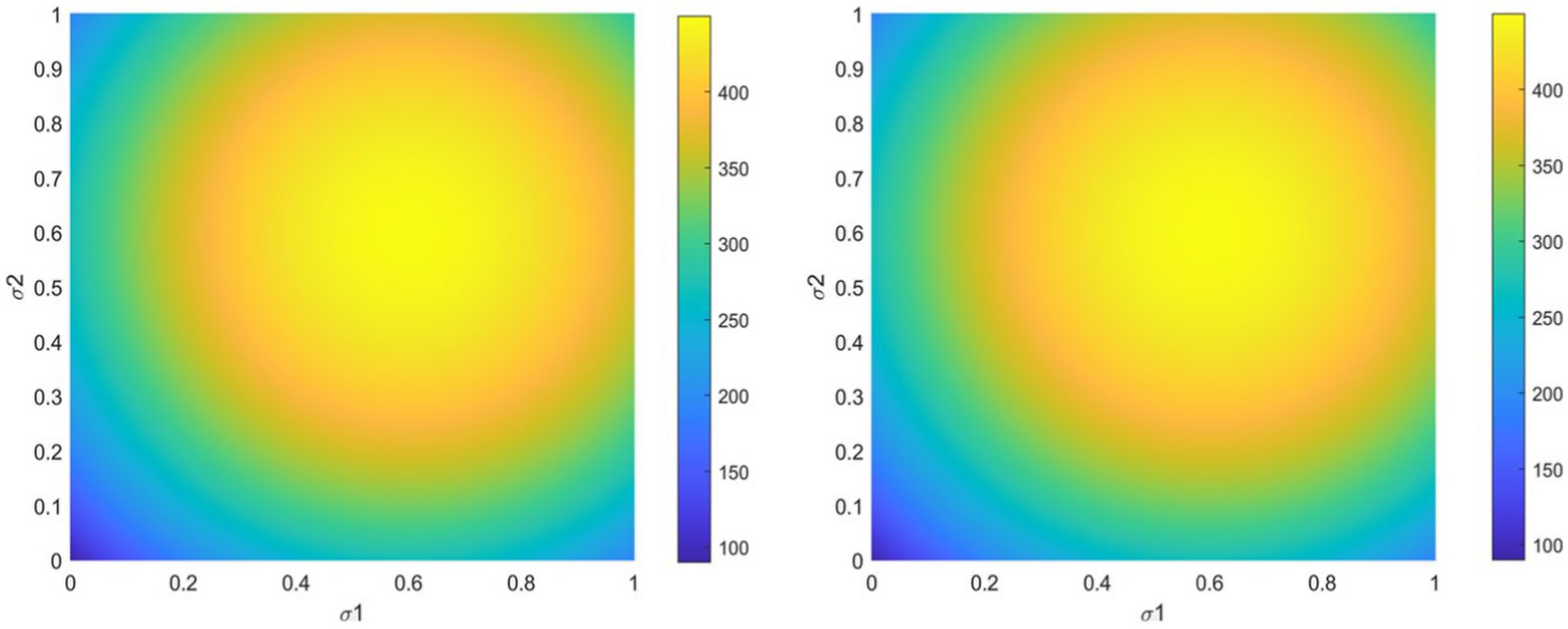
Figure 1. Variation of the profit for both firms in term of the OI rate of integration.

According to Figure 1, an interesting observation emerges: when both companies adopt a closed strategy at $100\%$ , their profits remain minimal. However, if one of them chooses to increase its open innovation (OI) integration rate, this positively influences the profits of both companies, causing them to grow. It is noteworthy that maximum profit for both companies requires an OI integration with a rate between $0.3$ and $0.7$ . However, exceeding this degree of integration leads to a negative impact on their profits, decreasing them. This observation underscores the crucial importance of finding an optimal balance in OI integration to maximize profits. Therefore, to gain a deeper understanding of this dynamics, we focus on studying the evolution of OI integration rates, ${\sigma }_1$ and ${\sigma }_2$ , around equilibrium $E_3$ . This thorough analysis will enable us to grasp how companies’ strategic decisions in the realm of open innovation affect their competitive performance.

5.1 Dynamics around $E_3$

By substituting the parameters from Table 1 into Equation (28), the Jacobian matrix will take the following form.

$J\left(E_3\right)=\left(\begin{array}{cc}\hfill 0.7\hfill & \hfill 0.3\hfill \\ \hfill 0.4\hfill & \hfill 0.5\hfill \end{array}\right)$

Table 1

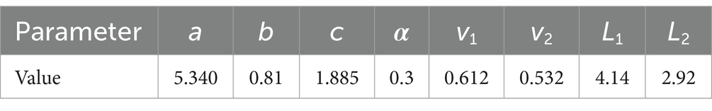
Table 1. Set of parameters used for the numerical simulation.

And its eigenvalues are: ${\lambda }_1=0.5<1$ and ${\lambda }_2=0.8<1$ , so $E_3$ is a stable point. We notice that the Jury conditions are verified, which means that the system is locally asymptotically stable around $E_3$ . Indeed

$\begin{array}{c}\hfill 1-Tr+det=0.1>0\hfill \\ \hfill 1+Tr+det=2.5>0\hfill \\ \hfill 1-det=0.7>0\hfill \end{array}$

These numerical results are illustrated graphically in the following figure, composed of two separate graphs. The first graph presents the trajectory of variation of ${\sigma }_1$ and ${\sigma }_2$ over time. We initialized the strategies of the two companies with an OI integration rate $\left({\sigma }_{1_0}\text{,}{\sigma }_{2_0}\right)=\left(0.4,0.4\right)$ . We observe that the solution oscillates slightly for about $35$time units before converging to the $E_3$ equilibrium. This dynamic is presented differently in the second graph, which represents the phase portrait showing the variation of ${\sigma }_1$ as a function of ${\sigma }_2$ . We notice that the trajectory oscillates until it converges toward the $E_3$ equilibrium, thus highlighting the stability of the system in the long term (Figure 2).

Figure 2

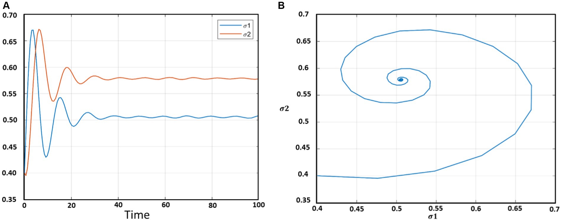
Figure 2. (A) Temporal variation of σ₁ and σ₂. (B) The phase plane of system around the equilibrium point.

Continuing our analysis, we seek to explore the impact of the variation of the parameters $L_1$ , $L_2$ and $\alpha$ on the stability of the system. This approach aims to determine to what extent the two companies can integrate intellectual property to benefit from the revenues it generates, while preserving the effectiveness of their cooperation strategies in the form of open innovation (OI). By studying the effect of these parameters on system stability, we will be able to identify the optimal intellectual property integration thresholds that allow companies to maximize their gains without compromising their IO collaboration. This in-depth analysis will provide a valuable resource to guide companies’ strategic decisions in the management of their intellectual property and their participation in open innovation networks, thereby promoting their long-term competitiveness in the market.

5.2 Impact of license prices L1 and L2

The first aspect of intellectual property lies in the sale of patent licenses at a given price. An increase in this price is a means to increase the revenues of both companies. However, it can also influence their open innovation strategy. Therefore, it is essential to determine the ranges in which license prices can be chosen for both companies. With this in mind, we construct the following bifurcation diagrams, illustrating the impact of varying $L_1$ , on ${\sigma }_2$ and $L_2$ on ${\sigma }_1$ . These diagrams will allow us to better understand the relationships between patent license prices and companies’ open innovation integration decisions, providing valuable insights for the strategic management of intellectual property and innovation initiatives (Figure 3).

Figure 3

Figure 3. Bifurcation diagram with respect to L₁ and L₂. (A) Firm 1, (B) Firm 2.

In the previous diagrams, we varied the parameters $L_1$ and $L_2$ in the interval [0,7]. We observe that an increase in the license price $L_2$ , ranging from 0 to slightly below 1.5, does not affect the stability of the system, and ${\sigma }_1$ remains constant without any apparent disturbance. This suggests that both companies maintain their open innovation strategies despite the increase in license prices. However, when $L_2$ exceeds $1.5$ , the system undergoes a bifurcation that results in a disturbance at the level of strategy ${\sigma }_1$ . This disturbance destabilizes the companies’ strategies, as the dynamics of the strategies are interdependent. Thus, a disturbance at the level of one strategy disrupts the entire system. Similarly, in the second diagram, the system remains stable as long as $L_1<1.3,$ but it loses its stability if $L_1$ exceeds this value.

In conclusion, the stability regions map as a function of $L_1$ and $L_2$ is plotted as shown by Figure 4. The green areas indicate stable regions, where for all values of $L_1$ and $L_2$ within this zone, the strategies of both companies are stable, meaning that the companies can adopt them. Conversely, the red zone represents unstable regions, where ${\sigma }_1$ and ${\sigma }_2$ never converge to a stable equilibrium. These regions should therefore be avoided in the choice of prices. Finally, the blue curve represents the bifurcation line, which marks the transition boundary between stable and unstable states of the system. This analysis allows us to delineate the domains in which patent license prices can be set to maintain the stability of companies’ open innovation strategies, while avoiding unstable areas where strategies may lose their effectiveness.

Figure 4

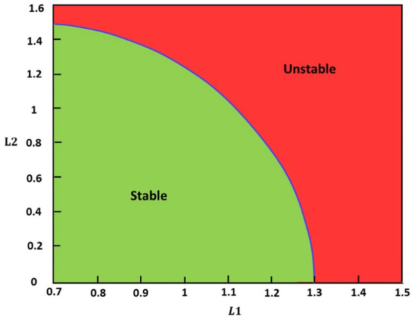
Figure 4. Stability regions.

5.3 Impact of royalty $\alpha$

In this section, the impact of the second component of intellectual property, namely the royalty $\alpha$ is analyzed. Similarly, we seek to determine the amount of money paid by one company to another for the use or exploitation of intellectual property, without it influencing the stability of open innovation (OI) strategies. To achieve this, we present the following two diagrams, which will allow us to visualize and understand how variations in royalty $\alpha$ affect the dynamics of companies’ OI strategies (Figure 5).

Figure 5

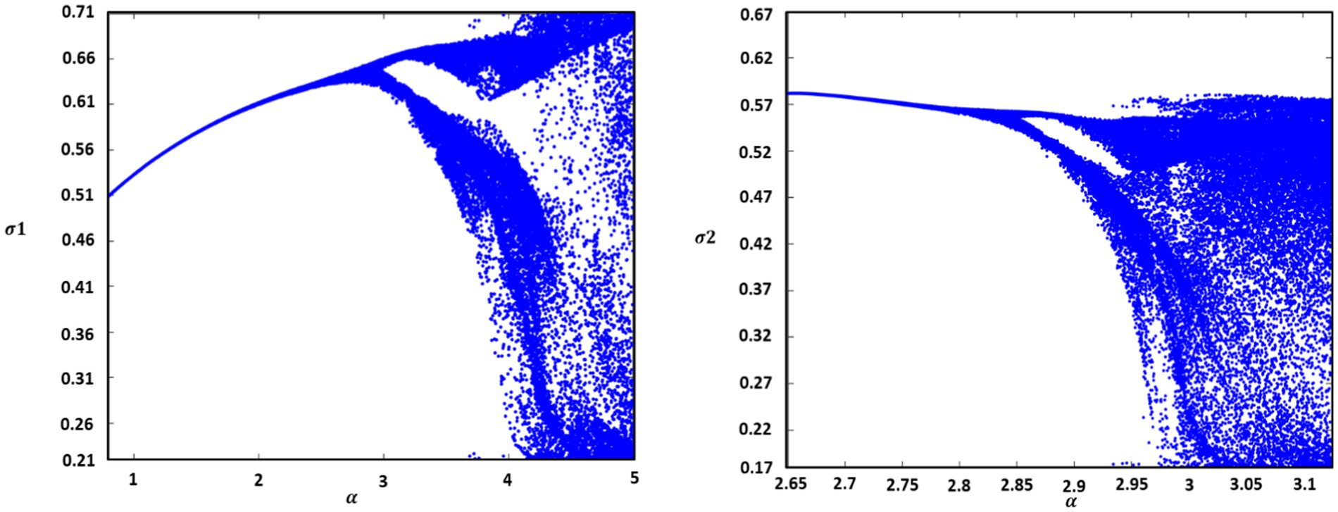
Figure 5. Bifurcation diagram with respect to α.

In these two diagrams, we varied $\alpha$ between 0 and 5. We observe that its effect is similar for ${\sigma }_1$ and ${\sigma }_2$ . As long as alpha is less than $2.85$ , the system maintains its stability. However, beyond this critical value of $2.85$ , the system undergoes a bifurcation and loses its stability. This observation underscores the importance of carefully choosing the value of royalty $\alpha$ to preserve the stability of companies’ open innovation strategies. A cautious adjustment of the royalty can thus reconcile the financial interests associated with the use of intellectual property with the need to maintain effective and stable open innovation strategies.

In this section, we have explored the crucial impact of parameters $L_1$ , $L_2$ , and $\alpha$ on the integration of intellectual property (IP) without compromising the open innovation (OI) strategies of competing companies. We have observed that the choice of patent license prices ( $L_1$ and $L_2$ ) and royalty $\alpha$ can have a significant effect on the stability of OI strategies. By varying these parameters within a given range, we have identified critical thresholds beyond which the system loses its stability, thereby compromising the OI strategies of companies. These results underscore the crucial importance of carefully choosing IP parameters to maximize revenue without disrupting companies’ OI strategies. Prudent management of these parameters can help reconcile the financial interests associated with IP use with the need to maintain effective and stable OI strategies, thus enhancing long-term competitiveness in the market.

6 Conclusion

In this study, we have examined profit maximization in a duopoly market where two competing firms operate. Using game theory, specifically the Cournot model, we investigated optimal strategies for these firms. Our research also delved into the avenue of collaboration through open innovation, aiming to delineate the best strategy for these players. We found that openness to innovation at a specific, though not complete, level was most effective. Beyond strategy analysis, we also studied the introduction of intellectual property in this context, utilizing bifurcation theory to assess its impacts on the equilibrium of firm strategies. Our findings highlight the importance of carefully managing intellectual property parameters to optimize revenue while maintaining the stability of open innovation strategies. These conclusions offer valuable insights for decision-makers, helping them in navigating a complex commercial landscape while capitalizing on the opportunities presented by innovation and intellectual property. In summary, our study provides a comprehensive analysis of competitive dynamics and the adaptive strategies necessary to thrive in an ever-evolving economic environment.

Data availability statement

The original contributions presented in the study are included in the article/supplementary material, further inquiries can be directed to the corresponding author.

Author contributions

AE: Conceptualization, Investigation, Methodology, Writing – original draft. AB: Conceptualization, Methodology, Writing – original draft, Writing – review & editing. MH: Resources, Supervision, Writing – original draft. JA: Project administration, Supervision, Visualization, Writing – original draft.

Funding

The author(s) declare that no financial support was received for the research, authorship, and/or publication of this article.

Conflict of interest

The authors declare that the research was conducted in the absence of any commercial or financial relationships that could be construed as a potential conflict of interest.

Publisher’s note

All claims expressed in this article are solely those of the authors and do not necessarily represent those of their affiliated organizations, or those of the publisher, the editors and the reviewers. Any product that may be evaluated in this article, or claim that may be made by its manufacturer, is not guaranteed or endorsed by the publisher.

References

1. Chu, Y. Y., and Liu, K. H. (2023). Managing open innovation challenges: Implementing organizational ambidextrous as a managerial approach. AIP Conference Proceedings.

Google Scholar

2. Mathurotpreechakun, W, and Torpanyacharn, K. Open innovation promoting with co-ownership of patent. Kasetsart J Soc Sci. (2023) 44, 321–326. doi: 10.34044/j.kjss.2023.44.2.01

Crossref Full Text | Google Scholar

3. Musiza, C . Weaving gender in open collaborative innovation, traditional cultural expressions, and intellectual property: the case of the Tonga baskets of Zambia. Int J Cult Prop. (2022) 29. doi: 10.1017/S0940739122000042

Crossref Full Text | Google Scholar

4. Osorno, R, and Medrano, N. Open innovation platforms: a conceptual design framework. IEEE Trans Eng Manag. (2022) 69:3227. doi: 10.1109/TEM.2020.2973227

Crossref Full Text | Google Scholar

5. Zhu, H, Lee, J, Yin, X, and Du, M. The effect of open innovation on manufacturing firms’ performance in China: the moderating role of social capital. Sustainability. (2023) 15:5854. doi: 10.3390/su15075854

Crossref Full Text | Google Scholar

6. Kunz, R . Open innovation in the life science industry In: Management for Professionals (2022) 169–184.

Google Scholar

7. Ozmel, U, Yavuz, D, Reuer, JJ, and Zenger, T. Network prominence, bargaining power, and the allocation of value capturing rights in high-tech alliance contracts. Organ Sci. (2017) 28:1147. doi: 10.1287/orsc.2017.1147

Crossref Full Text | Google Scholar

8. Pitkethly, RH . Intellectual property strategy in Japanese and UK companies: patent licensing decisions and learning opportunities. Res Policy. (2001) 30:425–42. doi: 10.1016/S0048-7333(00)00084-6

Crossref Full Text | Google Scholar

9. Alsaleh, M, and Abdul-Rahim, AS. The impacts of intellectual capital, market size, and intellectual property factors in geothermal power exploration. Energy Exploration Exploitation. (2024). doi: 10.1177/01445987231200100

Crossref Full Text | Google Scholar

10. Greco, M, Cricelli, L, Grimaldi, M, Strazzullo, S, and Ferruzzi, G. Unveiling the relationships among intellectual property strategies, protection mechanisms and outbound open innovation. Creat Innov Manag. (2022) 31:12498. doi: 10.1111/caim.12498

Crossref Full Text | Google Scholar

11. Grimaldi, M, Greco, M, and Cricelli, L. A framework of intellectual property protection strategies and open innovation. J Bus Res. (2021) 123:43. doi: 10.1016/j.jbusres.2020.09.043

Crossref Full Text | Google Scholar

12. Nguyen, TPT, Nguyen, TPT, and Tian, X. Intellectual property protection need as a driver for open innovation: empirical evidence from Vietnam. Technovation. (2023) 123:102714. doi: 10.1016/j.technovation.2023.102714

Crossref Full Text | Google Scholar

13. Arunnima, BS, Bijulal, D, and Sudhir Kumar, R. Open innovation intellectual property risk maturity model: an approach to measure intellectual property risks of software firms engaged in open innovation. Sustainability. (2023) 15:1036. doi: 10.3390/su151411036

Crossref Full Text | Google Scholar

14. Khouilla, H, and Bastidon, C. Does increased intellectual property rights protection foster innovation in developing countries? A literature review of innovation and catch-up. J Int Dev. (2024) 36:1170–88. doi: 10.1002/JID.3844

Crossref Full Text | Google Scholar

15. Li, Y, Zhang, Y, Hu, J, and Wang, Z. Insight into the nexus between intellectual property pledge financing and enterprise innovation: a systematic analysis with multidimensional perspectives. Int Rev Econ Finan. (2024) 93:700–19. doi: 10.1016/J.IREF.2024.03.050

Crossref Full Text | Google Scholar

16. Chu, T, and Zhou, W. Complex dynamics of R&D competition with one-way spillover based on intellectual property protection. Chaos Solitons Fractals. (2022) 163:112491. doi: 10.1016/J.CHAOS.2022.112491

Crossref Full Text | Google Scholar

17. Ikeda, T, Tanno, T, and Yasaki, Y. Optimal intellectual property rights policy by an importing country. Econ Lett. (2021) 209:110113. doi: 10.1016/j.econlet.2021.110113

Crossref Full Text | Google Scholar

18. Zhang, Y, Fan, R, Luo, M, Chen, M, and Sun, J. Evolutionary game analysis of firms’ technological strategic choices: a perspective of the behavioral biases. Complexity. (2021) 2021:1–17. doi: 10.1155/2021/4294125

Crossref Full Text | Google Scholar

19. Xing, M. (2010). The quantity competition between open source and proprietary software. Proceedings – 3rd International Conference on Information Management, Innovation Management and Industrial Engineering, ICIII 2010.

Google Scholar

20. Vivona, R, Demircioglu, MA, and Audretsch, DB. The costs of collaborative innovation. J Technol Transf. (2023) 48, 873–899. doi: 10.1007/s10961-022-09933-1

Crossref Full Text | Google Scholar

21. Elmire, A, Bassou, AA, Hlyal, M, and El Alami, J. Game theory approach for open innovation systems analysis in duopolistic market. Int J Adv Comput Sci Appl. (2023) 14:557–65. doi: 10.14569/IJACSA.2023.0140559

Crossref Full Text | Google Scholar

22. Casciato, DJ, Page, T, Perkins, J, Vacketta, V, and Hyer, C. Intellectual property and royalty payments among foot and ankle surgery fellowship faculty. J Foot Ankle Surg. (2023) 62:8. doi: 10.1053/j.jfas.2023.06.008

Crossref Full Text | Google Scholar

23. Chesbrough, H . The logic of open innovation. Calif Manag Rev. (2003) 45:33–58. doi: 10.1177/000812560304500301

Crossref Full Text | Google Scholar

24. Satoh, A, and Tanaka, Y. Choice of strategic variables under relative profit maximization in asymmetric oligopoly: non-equivalence of price strategy and quantity strategy. Econ Bus Lett. (2014) 3:115–26. doi: 10.17811/EBL.3.2.2014.115-126

Crossref Full Text | Google Scholar

25. Askar, SS, and Al-khedhairi, A. Dynamic investigations in a duopoly game with price competition based on relative profit and profit maximization. J Comput Appl Math. (2020) 367:112464. doi: 10.1016/J.CAM.2019.112464

Crossref Full Text | Google Scholar

26. Billette de Villemeur, E, Ruble, R, and Versaevel, B. Dynamic competition and intellectual property rights in a model of product development. J Econ Dyn Control. (2019) 100:270–96. doi: 10.1016/J.JEDC.2018.11.009

Crossref Full Text | Google Scholar

27. Bischi, GI, and Naimzada, A. Global analysis of a dynamic duopoly game with bounded rationality. Adv Dyn Games Appl. (2000):361–85. doi: 10.1007/978-1-4612-1336-9_20

Crossref Full Text | Google Scholar

28. Cao, Y, Colucci, R, and Guerrini, L. On the stability analysis of a delayed two-stage Cournot model with R&D spillovers. Math Comput Simul. (2022) 201:543–54. doi: 10.1016/J.MATCOM.2021.03.007

Crossref Full Text | Google Scholar

29. Dieci, R, and Westerhoff, F. Heterogeneous speculators, endogenous fluctuations and interacting markets: a model of stock prices and exchange rates. J Econ Dyn Control. (2010) 34:743–64. doi: 10.1016/J.JEDC.2009.11.002

Crossref Full Text | Google Scholar

30. Kopel, M, Westerhoff, F, and Wieland, C. Regulating complex dynamics in firms and economic systems. Chaos Solitons Fractals. (2008) 38:911–9. doi: 10.1016/J.CHAOS.2007.01.015

Crossref Full Text | Google Scholar

31. Askar, SS, Alshamrani, AM, and Alnowibet, K. Dynamic Cournot duopoly games with nonlinear demand function. Appl Math Comput. (2015) 259:427–37. doi: 10.1016/J.AMC.2015.02.072

Crossref Full Text | Google Scholar

32. Chen, J, Liang, L, and Yao, DQ. An analysis of intellectual property licensing strategy under duopoly competition: component or product-based? Int J Prod Econ. (2017) 193:502–13. doi: 10.1016/J.IJPE.2017.08.016

Crossref Full Text | Google Scholar

33. Yang, Z, Shi, Y, and Li, Y. Analysis of intellectual property cooperation behavior and its simulation under two types of scenarios using evolutionary game theory. Comput Ind Eng. (2018) 125:739–50. doi: 10.1016/J.CIE.2018.02.040

Crossref Full Text | Google Scholar