Qualitative properties of solutions to a nonlinear transmission problem for an elastic Bresse beam

We consider a nonlinear transmission problem for a Bresse beam, which consists of two parts, damped and undamped. The mechanical damping in the damping part is present in the shear angle equation only, and the damped part may be of arbitrary positive length. We prove the well-posedness of the corresponding system in energy space and establish the existence of a regular global attractor under certain conditions on the nonlinearities and coefficients of the damped part only. Besides, we study the singular limits of the problem under consideration when curvature tends to zero, or curvature tends to zero, and simultaneously shear moduli tend to infinity and perform numerical modeling for these processes.

1 Introduction

In this study, we consider a contact problem for the Bresse beam. Originally, the mathematical model for homogeneous Bresse beams was derived in Ref. [1]. We use the variant of the model described in Ref. [2, Ch. 3]. Let the whole beam occupy a part of a circle of length L and have the curvature l = R⁻¹. We consider the beam as a one-dimensional object and measure the coordinate x along the beam. Thus, we say that the coordinate x changes within the interval (0, L). The parts of the beam occupying the intervals (0, L₀) and (L₀, L) consist of different materials. The part lying in the interval (0, L₀) is partially subjected to structural damping (see Figure 1). The Bresse system describes the evolution of three quantities: transversal displacement, longitudinal displacement, and shear angle variation. We denote by φ, ψ, and ω the transversal displacement, the shear angle variation, and the longitudinal displacement of the left part of the beam lying in (0, L₀). Analogously, we denote by u, v, and w the transversal displacement, the shear angle variation, and the longitudinal displacement of the right part of the beam occupying the interval (L₀, L). We assume the presence of mechanical dissipation in the equation for the shear angle variation for the left part of the beam. We also assume that both ends of the beam are fixed. Nonlinear oscillations of the composite beam can be described by the following equation system:

$\begin{array}{ll}{\rho }_1{\phi }_{tt}-k_1{({\phi }_x+\psi +l\omega )}_x-l{\sigma }_1({\omega }_x-l\phi )+f_1(\phi ,\psi ,\omega )=p_1(x,t),& (1)\end{array}$

$\begin{array}{ll}{\beta }_1{\psi }_{tt}-{\lambda }_1{\psi }_{xx}+k_1({\phi }_x+\psi +l\omega )+\gamma ({\psi }_t)+h_1(\phi ,\psi ,\omega )=r_1(x,t),x\in (0,L_0),t>0,& (2)\end{array}$

$\begin{array}{ll}{\rho }_1{\omega }_{tt}-{\sigma }_1{({\omega }_x-l\phi )}_x+l{k}_1({\phi }_x+\psi +l\omega )+g_1(\phi ,\psi ,\omega )=q_1(x,t),& (3)\end{array}$

Figure 1

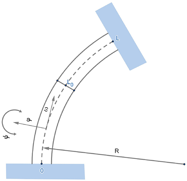
Figure 1. Composite Bresse beam.

and

$\begin{array}{ll}{\rho }_2{u}_{tt}-k_2{(u_x+v+lw)}_x-l{\sigma }_2(w_x-lu)+f_2(u,v,w)=p_2(x,t),& (4)\end{array}$

$\begin{array}{l}{\beta }_2{v}_{tt}-{\lambda }_2{v}_{xx}+k_2(u_x+v+lw)+h_2(u,v,w)=r_2(x,t),\\ x\in (L_0,L),t>0,& (5)\end{array}$

$\begin{array}{ll}{\rho }_2{w}_{tt}-{\sigma }_2{(w_x-lu)}_x+l{k}_2(u_x+v+lw)+g_2(u,v,w)=q_2(x,t),& (6)\end{array}$

where ρ_j, β_j, k_j, σ_j, λ_j are positive parameters, $f_j,g_j,h_j:{ℝ}^3\to ℝ$ are nonlinear feedbacks, $p_j,q_j,r_j:(0,L)\times {ℝ}^3\to ℝ$ are known external loads and γ:ℝ → ℝ is a nonlinear damping. The system is subjected to Dirichlet boundary conditions at the ends of the beam

$\begin{array}{ll}\begin{array}{c}\phi (0,t)=u(L,t)=0,\psi (0,t)=v(L,t)=0,\\ \omega (0,t)=w(L,t)=0,\end{array}& (7)\end{array}$

transmission conditions at point L₀

$\begin{array}{ll}\phi (L_0,t)=u(L_0,t),\psi (L_0,t)=v(L_0,t),\omega (L_0,t)=w(L_0,t),& (8)\end{array}$

$\begin{array}{ll}{k}_1({\phi }_x+\psi +l\omega )(L_0,t)=k_2(u_x+v+lw)(L_0,t),& (9)\end{array}$

$\begin{array}{ll}{\lambda }_1{\psi }_x(L_0,t)={\lambda }_2{v}_x(L_0,t),& (10)\end{array}$

$\begin{array}{ll}{\sigma }_1({\omega }_x-l\phi )(L_0,t)={\sigma }_2(w_x-lu)(L_0,t),& (11)\end{array}$

and supplemented with the initial conditions

$\begin{array}{ll}\phi (x,0)={\phi }_0(x),\psi (x,0)={\psi }_0(x),\omega (x,0)={\omega }_0(x),& (12)\end{array}$

$\begin{array}{ll}{\phi }_t(x,0)={\phi }_1(x),{\psi }_t(x,0)={\psi }_1(x),{\omega }_t(x,0)={\omega }_1(x),& (13)\end{array}$

$\begin{array}{ll}u(x,0)=u_0(x),v(x,0)=v_0(x),w(x,0)=w_0(x),& (14)\end{array}$

$\begin{array}{ll}{u}_t(x,0)=u_1(x),v_t(x,0)=v_1(x),w_t(x,0)=w_1(x).& (15)\end{array}$

One can observe patterns in the problem that appear to have physical meaning:

$\begin{array}{l}{Q}_i(\xi ,\zeta ,\eta )=k_i({\xi }_x+\zeta +l\eta )\text{ are shear forces},\\ N_i(\xi ,\zeta ,\eta )={\sigma }_i({\eta }_x-l\xi )\text{ are axial forces }\text{and}\\ M_i(\xi ,\zeta ,\eta )={\lambda }_i{\zeta }_x\text{ are bending moments}\end{array}$

for damped (i = 1) and undamped (i = 2) parts. Later we will use them to rewrite the problem in a compact and physically natural form.

This study is devoted to the well-posedness and long-time behavior of the system (1)–(15). Our main goal is to establish conditions under which the assumed amount of dissipation is sufficient to guarantee the existence of a global attractor.

The study is organized as follows: In Section 2, we represent functional spaces and pose the problem in an abstract form. In Section 3, we prove that the problem is well-posed and possesses strong solutions, provided nonlinearities, and initial data are smooth enough. Section 4 is devoted to the main result of the existence of a compact attractor. The nature of dissipation prevents us from proving dissipativity explicitly; thus, we show that the corresponding dynamical system is of gradient structure and asymptotically smooth. We establish the unique continuation property applying the Carleman estimate obtained in Ref. [3] to prove the gradient property. The compensated compactness approach is used to prove asymptotic smoothness. In Section 5, we show that solutions to (1)–(15) tend to solutions to a transmission problem for the Timoshenko beam when l → 0 and to solutions to a transmission problem for the Kirchhoff beam with rotational inertia when l → 0 and k_i → ∞, as well as perform numerical modeling of these singular limits.

2 Preliminaries and abstract formulation

2.1 Spaces and notations

Let us denote

$\begin{array}{l}{\Phi }^1=(\phi ,\psi ,\omega ),{\Phi }^2=(u,v,w),\Phi =({\Phi }^1,{\Phi }^2).\end{array}$

Thus, Φ is a six-dimensional vector of functions. Analogously,

$\begin{array}{l}{F}_j=(f_j,g_j,h_j):{ℝ}^3\to {ℝ}^3,F=(F_1,F_2),\\ P_j=(p_j,q_j,r_j):{\left[(0,L)\times {ℝ}_{+}\right]}^3\to {ℝ}^3,P=(P_1,P_2),\\ R_j=diag\left\{{\rho }_j,{\beta }_j,{\rho }_j\right\},R=diag\left\{{\rho }_1,{\beta }_1,{\rho }_1,{\rho }_2,{\beta }_2,{\rho }_2\right\}\text{and}\\ \Gamma ({\Phi }_t)=(0,\gamma ({\psi }_t),0,0,0,0),\end{array}$

where j = 1, 2. The static linear part of the equation system can be formally rewritten as

$\begin{array}{ll}A\Phi =\left(\begin{array}{c}-{\partial }_x{Q}_1({\Phi }^1)-l{N}_1({\Phi }^1)\\ -{\partial }_x{M}_1({\Phi }^1)+Q_1({\Phi }^1)\\ -{\partial }_x{N}_1({\Phi }^1)+l{Q}_1({\Phi }^1)\\ -{\partial }_x{Q}_2({\Phi }^2)-l{N}_2({\Phi }^2)\\ -{\partial }_x{M}_2({\Phi }^2)+Q_2({\Phi }^2)\\ -{\partial }_x{N}_2({\Phi }^2)+l{Q}_2({\Phi }^2)\end{array}\right).& (16)\end{array}$

Then transmission conditions (8)–(11) can be written as follows:

$\begin{array}{l}{\Phi }^1(L_0,t)={\Phi }^2(L_0,t),\\ Q_1({\Phi }^1(L_0,t))=Q_2({\Phi }^2(L_0,t)),\\ M_1({\Phi }^1(L_0,t))=M_2({\Phi }^2(L_0,t)),\\ N_1({\Phi }^1(L_0,t))=N_2({\Phi }^2(L_0,t)).\end{array}$

Throughout the study, we use the notation ||·|| for the L²-norm of a function and (·, ·) for the L²-inner product. In these notations, we skip the domain on which functions are defined. We adopt the notation $\left|\right|·|{|}_{L^2(\Omega )}$ only when the domain is not evident. We also use the same notations ||·|| and (·, ·) for [L²(Ω)]³.

To write our problem in an abstract form form, introduce the following spaces: For the velocities of the displacements, we use the space

$\begin{array}{l}{H}_v=\{\Phi =({\Phi }^1,{\Phi }^2):{\Phi }^1\in {[L^2(0,L_0)]}^3,{\Phi }^2\in {[L^2(L_0,L)]}^3\}\end{array}$

with the norm

$\begin{array}{l}\left|\right|\Phi |{|}_{H_v}^2=||\Phi |{|}_v^2={\displaystyle \sum _{j=1}^2}\left|\right|\sqrt{R_j}{\Phi }^j|{|}^2,\end{array}$

which is equivalent to the standard L²-norm.

For the beam displacements, use the space

$\begin{array}{l}{H}_d=\{\Phi \in H_v:{\Phi }^1\in {[H^1(0,L_0)]}^3,{\Phi }^2\in {[H^1(L_0,L)]}^3,\\ {\Phi }^1(0,t)={\Phi }^2(L,t)=0,{\Phi }^1(L_0,t)={\Phi }^2(L_0,t)\}\end{array}$

with the norm

$\begin{array}{l}\left|\right|\Phi |{|}_{H_d}^2=||\Phi |{|}_d^2={\displaystyle \sum _{j=1}^2}(\left|\right|Q_j({\Phi }^j)|{|}^2+|\left|N_j({\Phi }^j)\right|{|}^2+\left|\right|M_j({\Phi }^j)|{|}^2).\end{array}$

This norm is equivalent to the standard H¹-norm. Moreover, the equivalence constants can be chosen independent of l for l is small enough (see Ref. [4], Remark 2.1). If we set

$\begin{array}{l}\text{Ψ}(x)=\{\begin{array}{cc}{\Phi }^1(x),& x\in (0,L_0),\\ {\Phi }^2(x),& x\in [L_0,L)\end{array}\end{array}$

we see that there is an isomorphism between H_d and ${\left[H_0^1(0,L)\right]}^3$.

2.2 Abstract formulation

The operator A : D(A) ⊂ H_v → H_v is defined by formula (16), where

$\begin{array}{c}D(A)=\{\Phi \in H_d:{\Phi }^1\in H^2(0,L_0),{\Phi }^2\in H^2(L_0,L),\\ Q_1({\Phi }^1(L_0,t))=Q_2({\Phi }^2(L_0,t)),\\ N_1({\Phi }^1(L_0,t))=N_2({\Phi }^2(L_0,t)),M_1({\Phi }^1(L_0,t))=M_2({\Phi }^2(L_0,t))\}.\end{array}$

Arguing analogously to Lemmas 1.1-1.3 from Ref. [5], one can prove the following lemma.

Lemma 2.1. The operator A is positive and self-adjoint. Moreover,

$\begin{array}{l}\begin{array}{l}(A^{1/2}\Phi ,A^{1/2}B)=\frac{1}{k_1}(Q_1({\Phi }^1),Q_1(B^1))+\frac{1}{{\sigma }_1}(N_1({\Phi }^1),N_1(B^1))\\ +\frac{1}{{\lambda }_1}(M_1({\Phi }^1),M_1(B^1))\\ +\frac{1}{k_2}(Q_2({\Phi }^2),Q_2(B^2))+\frac{1}{{\sigma }_2}(N_2({\Phi }^2),N_2(B^2))\\ +\frac{1}{{\lambda }_2}(M_2({\Phi }^2),M_2(B^2))\end{array}\end{array}$

and $D(A^{1/2})=H_d\subset H_v$.

Thus, we can rewrite equations (1)–(6) in the form of

$\begin{array}{ll}R{\Phi }_{tt}+A\Phi +\Gamma ({\Phi }_t)+F(\Phi )=P(x,t),& (17)\end{array}$

boundary conditions (7) in the form of

$\begin{array}{ll}{\Phi }^1(0,t)={\Phi }^2(L,t)=0,& (18)\end{array}$

and transmission conditions (8)–(11) can be written as

$\begin{array}{ll}{\Phi }^1(L_0,t)={\Phi }^2(L_0,t),& (19)\end{array}$

$\begin{array}{ll}{Q}_1({\Phi }^1(L_0,t))=Q_2({\Phi }^2(L_0,t)),& (20)\end{array}$

$\begin{array}{ll}{M}_1({\Phi }^1(L_0,t))=M_2({\Phi }^2(L_0,t))\text{and}& (21)\end{array}$

$\begin{array}{ll}{N}_1({\Phi }^1(L_0,t))=N_2({\Phi }^2(L_0,t)).& (22)\end{array}$

Initial conditions have the form

$\begin{array}{ll}\Phi (x,0)={\Phi }_0(x)\text{and }{\Phi }_t(x,0)={\Phi }_1(x).& (23)\end{array}$

We use H = H_d × H_v as a phase space.

3 Well-posedness

In this section, we study strong, generalized, and variational (weak) solutions to (17)–(23).

Definition 3.1. $\Phi \in C(0,T;H_d)\bigcap C^1(0,T;H_v)$ such that Φ(x, 0) = Φ₀(x), Φ_t(x, 0) = Φ₁(x) is said to be a strong solution to (17)–(23), if

• Φ(t) lies in D(A) for almost all t;

• Φ(t) is continuous function with values in H_d and Φ_t ∈ L₁(a, b; H_d) for 0 < a < b < T;

• Φ_t(t) is continuous function with values in H_v and Φ_tt ∈ L₁(a, b; H_v) for 0 < a < b < T;

• Equation (17) is satisfied for almost all t and

Definition 3.2. $\Phi \in C(0,T;H_d)\bigcap C^1(0,T;H_v)$ such that Φ(x, 0) = Φ₀(x) and Φ_t(x, 0) = Φ₁(x) are said to be a generalized solution to (17)–(23), if there exists a sequence of strong solutions Φ⁽ⁿ⁾ to (17)–(23) with the initial data $({\Phi }_0^{(n)},{\Phi }_1^{(n)})$ and right hand side P⁽ⁿ⁾(x, t) such that

$\begin{array}{l}{\displaystyle \underset{n\to \infty }{lim}}{\displaystyle \underset{t\in \left[0,T\right]}{max}}\left(\left|\right|{\Phi }^{(n)}(·,t)-\Phi (·,t)|{|}_d+||{\Phi }_t^{(n)}(·,t)-{\Phi }_t(·,t)|{|}_v\right)=0.\end{array}$

We also need a definition of a variational solution. We use six-dimensional vector functions B = (B¹, B²), B^j = (β^j, γ^j, δ^j) from the space

$\begin{array}{l}{F}_T=\left\{B\in L^2(0,T;H_d),B_t\in L^2(0,T;H_v),B(T)=0\right\}\end{array}$

as test functions.

Definition 3.3. Φ is said to be a variational (weak) solution to (17)–(23) if

• $\Phi \in L^{\infty }(0,T;H_d),{\Phi }_t\in L^{\infty }(0,T;H_v)$;

• satisfy the following variational equality for all B ∈ F_T

$\begin{array}{l}-{\displaystyle \underset{0}{\overset{T}{\int }}}(R{\Phi }_t,B_t)(t)dt-(R{\Phi }_1,B(0))+{\displaystyle {\int }_0^T}(A^{1/2}\Phi ,A^{1/2}B)(t)dt+\\ {\displaystyle {\int }_0^T}(\Gamma ({\Phi }_t),B)(t)dt+{\displaystyle {\int }_0^T}(F(\Phi ),B)(t)dt-{\displaystyle {\int }_0^T}(P,B)(t)dt=0;& (24)\end{array}$

• Φ(x, 0) = Φ₀(x).

Now we state a well-posedness result for problems (17)–(23).

Theorem 3.4 (well-posedness). Let

$\begin{array}{l}{f}_i,g_i,h_i:{ℝ}^3\to ℝ\text{ are locally Lipschitz, i.e.,}\\ |f_i(a)-f_i(b)|\le L(K)|a-b|,\text{provided}\left|a\right|,\left|b\right|\le K;& (\mathrm{N1})\end{array}$

$\begin{array}{l}\text{there exists }{\mathcal{F}}_i:{ℝ}^3\to ℝ\text{ such that }(f_i,h_i,g_i)=\nabla {\mathcal{F}}_i;\\ \text{there exists }\delta >0\text{ such that }{\mathcal{F}}_j(a)\ge -\delta \text{ for all }a\in {ℝ}^3;& (\mathrm{N2})\end{array}$

$\begin{array}{ll}P\in L^2(0,T;H_v);& (\mathrm{R1})\end{array}$

and the nonlinear dissipation satisfies

$\begin{array}{ll}\gamma \in C(ℝ)\text{and non-decreasing }\gamma (0)=0.& (\mathrm{D1})\end{array}$

Then for every initial data Φ₀ ∈ H_d, Φ₁ ∈ H_v, and time interval [0, T], there exists a unique generalized solution to (17)–(23) with the following properties:

• every generalized solution is variational;

• energy inequality

$\begin{array}{ll}\mathcal{E}(T)+{\displaystyle {\int }_0^T}(\gamma ({\psi }_t),{\psi }_t)dt\le \mathcal{E}(0)+{\displaystyle {\int }_0^T}(P(t),{\Phi }_t(t))dt& (25)\end{array}$

holds, where

$\begin{array}{l}\mathcal{E}(t)=\frac{1}{2}\left[\left|\right|R^{1/2}{\Phi }_t(t)|{|}^2+||A^{1/2}\Phi (t)|{|}^2\right]+{\displaystyle \underset{0}{\overset{L}{\int }}}\mathcal{F}(\Phi (x,t))dx\end{array}$

and

$\begin{array}{l}\mathcal{F}(\Phi (x,t))=\{\begin{array}{cc}{\mathcal{F}}_1(\phi (x,t),\psi (x,t),\omega (x,t)),& x\in (0,L_0),\\ {\mathcal{F}}_2(u(x,t),v(x,t),w(x,t)),& x\in (L_0,L).\end{array}\end{array}$

• If, additionally, Φ₀ ∈ D(A), Φ₁ ∈ H_d and

$\begin{array}{ll}{\partial }_{t}P(x,t)\in L_2(0,T;H_v)& (\mathrm{R2})\end{array}$

then the generalized solution is also strong and satisfies the energy equality.

Proof. The proof essentially uses the monotone operator theory. It is rather standard by now (see e.g., Ref. [6]), so in some parts, we give only references to corresponding arguments. However, we give some details that demonstrate the peculiarities of 1D problems.

Step 1. Abstract formulation. We need to reformulate problems (17)–(23) as first-order problems. Let us denote

$\begin{array}{l}U=(\Phi ,{\Phi }_t),U_0=({\Phi }_0,{\Phi }_1)\in H=H_d\times H_v,\end{array}$

$\begin{array}{l}\mathcal{T}U=\left(\begin{array}{cc}I& 0\\ 0& R^{-1}\end{array}\right)\left(\begin{array}{cc}0& -I\\ A& 0\end{array}\right)U+\left(\begin{array}{c}0\\ \Gamma \left({\Phi }_t\right)\end{array}\right).\end{array}$

Consequently, $D\left(\mathcal{T}\right)=D\left(A\right)\times H_d\subset H$. In the proof, we denote

$\begin{array}{l}\mathcal{B}\left(U\right)=\left(\begin{array}{cc}I& 0\\ 0& R^{-1}\end{array}\right)\left(\begin{array}{c}0\\ F\left(\Phi \right)\end{array}\right),\mathcal{P}\left(x,t\right)=\left(\begin{array}{c}0\\ P\left(x,t\right)\end{array}\right).\end{array}$

Thus, we can rewrite problem (17)–(23) in the form

$\begin{array}{l}{U}_t+\mathcal{T}U+\mathcal{B}(U)=\mathcal{P},U(0)=U_0\in H.\end{array}$

Step 2. Existence and uniqueness of a local solution. Here, we use Theorem 7.2 from Ref. [6]. For the reader's convenience, we formulate it below.

Theorem 3.5 (Ref. [6]). Consider the initial value problem

$\begin{array}{ll}{U}_t+\mathcal{T}U+B(U)=f,U(0)=U_0\in H.& (26)\end{array}$

Suppose that $\mathcal{T}:D(\mathcal{T})\subset H\to H$ is a maximal monotone mapping, $0\in \mathcal{T}0$ and B:H → H is locally Lipschitz, i.e., there exits L(K) > 0 such that

$\begin{array}{l}\left|\right|B(U)-B(V)|{|}_H\le L(K)||U-V|{|}_H,\left|\right|U|{|}_H,|\left|V\right|{|}_H\le K.\end{array}$

If $U_0\in D(\mathcal{T})$, $f\in W_1^1(0,t;H)$ for all t > 0, then there exists t_max ≤ ∞ such that (26) has a unique strong solution U on (0, t_max).

If $U_0\in \overline{D(\mathcal{T})}$, f ∈ L¹(0, t; H) for all t > 0, then there exists t_max ≤ ∞ such that (26) has a unique generalized solution U on (0, t_max).

In both cases

$\begin{array}{l}{\displaystyle \underset{t\to t_{max}}{lim}}\left|\right|U(t)|{|}_H=\infty \text{provided }{t}_{max}<\infty .\end{array}$

First, we need to check that $\mathcal{T}$ is a maximal monotone operator. Monotonicity is a direct consequence of Lemma 2.1 and (D1).

To prove $\mathcal{T}$ is maximal as an operator from H to H, we use Theorem 1.2 from Ref. [7, Ch. 2]. Thus, we need to prove that $Range(I+\mathcal{T})=H$, with I being the duality map from H to H. Let z = (Φ_z, Ψ_z) ∈ H_d × H_v. We need to find $y=({\Phi }_y,{\text{Ψ}}_y)\in D(A)\times H_d=D(\mathcal{T})$ such that

$\begin{array}{l}-{\text{Ψ}}_y+{\Phi }_y={\Phi }_z,\\ A{\Phi }_y+{\text{Ψ}}_y+\Gamma ({\text{Ψ}}_y)={\text{Ψ}}_z,\end{array}$

or, equivalently, find Ψ_y ∈ H_d such that

$\begin{array}{l}M({\text{Ψ}}_y)=\frac{1}{2}A{\text{Ψ}}_y+\frac{1}{2}A{\text{Ψ}}_y+{\text{Ψ}}_y+\Gamma ({\text{Ψ}}_y)={\text{Ψ}}_z-A{\Phi }_z={\Theta }_z\end{array}$

for an arbitrary ${\Theta }_z\in H_d^{\prime }=D{(A^{1/2})}^{\prime }$. Naturally, due to Lemma 2.1, A is a duality map between H_d and $H_d^{\prime }$, thus the operator M is onto if and only if $\frac{1}{2}A{\text{Ψ}}_y+{\text{Ψ}}_y+\Gamma ({\text{Ψ}}_y)$ is maximal monotone as an operator from H_d to $H_d^{\prime }$. According to Corollary 1.1 from Ref. [7, Ch. 2], this operator is maximal monotone if $\frac{1}{2}A$ is maximal monotone (it follows from Lemma 2.1) and I + Γ(·) is monotone, bounded and hemicontinuous from H_d to $H_d^{\prime }$. The last statement is evident for the identity map; now let's prove it for Γ.

Monotonicity is evident here. Due to the continuity of the embedding $H^1(0,L_0)\subset C(0,L_0)$ in 1D, every bounded set X in $H^1(0,L_0)$ is bounded in C(0, L₀) and thus, due to (D1), Γ(X) is bounded in C(0, L₀) and, consequently, in $L^2(0,L_0)$. To prove hemicontinuity, we take an arbitrary Φ = (φ, ψ, ω, u, v, w) ∈ H_d and an arbitrary Θ = (θ₁, θ₂, θ₃, θ₄, θ₅, θ₆) ∈ H_d and consider

$\begin{array}{l}(\Gamma ({\text{Ψ}}_y+t\Phi ),\Theta )={\displaystyle {\int }_0^{L_0}}\gamma ({\psi }_y(x)+t\psi (x)){\theta }_2(x)dx,\end{array}$

where Ψ_y = (φ_y, ψ_y, ω_y, u_y, v_y, w_y). Since ψ_y + tψ → ψ_y, as t → 0 in $H^1(0,L_0)$ and in C(0, L₀), we obtain that γ(ψ_y(x)+tϕ(x)) → γ(ψ_y(x)) as t → 0 for every x ∈ [0, L₀], and has an integrable bound from above due to (D1). This implies γ(ψ_y(x)+tϕ(x)) → γ(ψ_y(x)) in $L^1(0,L_0)$ as t → 0. Since ${\theta }_2\in H^1(0,L_0)\subset L^{\infty }(0,L_0)$,

$\begin{array}{l}(\Gamma ({\text{Ψ}}_y+t\Phi ),\Theta )\to (\Gamma ({\text{Ψ}}_y),\Theta ),t\to 0.\end{array}$

Hemicontinuity is proved now.

Further, we need to prove that $\mathcal{B}$ is locally Lipschitz on H, i.e., F is locally Lipschitz from H_d to H_v. The embedding H^1/2+ε(0, L) ⊂ C(0, L) and (N1) imply

$\begin{array}{ll}|F_j({\tilde{\Phi }}^j(x))-F_j({\hat{\Phi }}^j(x))|\le C(max(\left|\right|\tilde{\Phi }|{|}_d,|\left|\hat{\Phi }\right|{|}_d))\left|\right|{\tilde{\Phi }}^j-{\hat{\Phi }}^j|{|}_1& (27)\end{array}$

for all x ∈ [0, L₀], if j = 1 and for all x ∈ [L₀, L], if j = 2. This, in turn, gives us the estimate

$\begin{array}{l}\left|\right|F(\tilde{\Phi })-F(\hat{\Phi })|{|}_v\le C(max(\left|\right|\tilde{\Phi }|{|}_d,|\left|\hat{\Phi }\right|{|}_d))||\tilde{\Phi }-\hat{\Phi }|{|}_d.\end{array}$

Thus, all the assumptions of Theorem 3.5 are satisfied and the existence of a local strong/generalized solution is proved.

Step 3. Energy inequality and global solutions. It can be verified by direct calculations, that strong solutions satisfy energy equality. Using the same arguments, as in the proof of Proposition 1.3 [8], and (D1) we can pass to the limit and prove (25) for generalized solutions.

Let us assume that a local generalized solution exists on a maximal interval (0, t_max), t_max < ∞. Then Equation (25) implies $\mathcal{E}(t_{max})\le \mathcal{E}(0)$. Since due to (N2)

$\begin{array}{l}{c}_1\left|\right|U(t)|{|}_H\le \mathcal{E}(t)\le c_2|\left|U(t)\right|{|}_H,\end{array}$

we have ||U(t_max)||_H ≤ C||U₀||_H. Thus, we arrive at a contradiction which implies t_max = ∞.

Step 4. The generalized solution is variational (weak). We formulate the following obvious estimate as a lemma for future use.

Lemma 3.6. Let (N1) hold and $\tilde{\Phi }$, $\hat{\Phi }$ are two weak solutions to (17)–(23) with the initial conditions $({\tilde{\Phi }}_0,{\tilde{\Phi }}_1)$ and $({\hat{\Phi }}_0,{\hat{\Phi }}_1)$ respectively. Then the following estimate is valid for all x ∈ [0, L], t > 0 and ϵ ∈ [0, 1/2):

$\begin{array}{l}|F_j({\tilde{\Phi }}^j(x,t))-F_j({\hat{\Phi }}^j(x,t))|\le C(max(\left|\right|({\tilde{\Phi }}_0,{\tilde{\Phi }}_1)|{|}_H,|\left|({\hat{\Phi }}_0,{\hat{\Phi }}_1)\right|{|}_H))\\ \hfill \left|\right|{\tilde{\Phi }}^j(·,t)-{\hat{\Phi }}^j(·,t)|{|}_{1-ϵ},j=1,2.\end{array}$

Proof. The energy inequality and the embedding H^1/2+ε(0, L) ⊂ C(0, L) imply that for every weak solution Φ

$\begin{array}{l}{\displaystyle \underset{t\in \left[0,T\right],x\in \left[0,L\right]}{max}}|\Phi (x,t)|\le C(\left|\right|{\Phi }_0|{|}_d,|\left|{\Phi }_1\right|{|}_v).\end{array}$

Thus, using (N1) and (27), we prove the lemma.

Evidently, Equation (24) is valid for strong solutions. We can find a sequence of strong solutions Φ⁽ⁿ⁾, which converges to a generalized solution Φ strongly in C(0, T; H_d), and ${\Phi }_t^{(n)}$ converges to Φ_t strongly in C(0, T; H_v). Using Lemma 3.6, we can easily pass to the limit in nonlinear feedback terms in (24). Since the test function $B\in L^{\infty }(0,T;H_d)\subset L^{\infty }((0,T)\times (0,L))$, we can use the same arguments as in the proof of Proposition 1.6 [8] to pass to the limit in the nonlinear dissipation term. Namely, we can extract from ${\Phi }_t^{(n)}$ a subsequence that converges to Φ_t almost everywhere and prove that it converges to Φ_t strongly in L¹((0, T) × (0, L)).

Remark 1. In space dimension greater than one we do not have the embedding H¹(Ω) ⊂ C(Ω), therefore we need to assume polynomial growth of the derivative of the nonlinearity to obtain estimates similar to Lemma 3.6.

4 Existence of attractors

In this section, we study the long -time behavior of solutions to problems (17)–(23) in the framework of dynamical systems theory. From Theorem 3.4, we have

Corollary 1. In addition to the conditions of Theorem 3.4, let P(x, t) = P(x). Then (17)–(23) generates a dynamical system (H, S_t) by using the formula

$\begin{array}{l}{S}_t({\Phi }_0,{\Phi }_1)=(\Phi (t),{\Phi }_t(t)),\end{array}$

where Φ(t) is the weak solution to (17)–(23) with initial data (Φ₀, Φ₁).

To establish the existence of the attractor for this dynamical system, we use Theorem 4.8 below; thus, we need to prove the gradientness, the asymptotic smoothness, as well as the boundedness of the set of stationary points.

4.1 Gradient structure

In this subsection, we prove that the dynamical system generated by (17)–(23) possesses a specific structure, namely, a gradient under some additional conditions on the nonlinearities.

Definition 4.1 (Ref. [9–11]). Let Y ⊆ X be a positively invariant set of (X, S_t).

• a continuous functional L(y), defined on Y, is said to be a Lyapunov function of the dynamical system (X, S_t) on the set Y if a function t ↦ L(S_ty) is non-increasing for any y ∈ Y.

• the Lyapunov function L(y) is said to be strict on Y if the equality L(S_ty) = L(y) for all t > 0 implies S_ty = y for all t > 0;

• a dynamical system (X, S_t) is said to be gradient if it possesses a strict Lyapunov function on the whole phase space X.

The following result holds true:

Theorem 4.2. Let, additionally to the assumptions of Corollary 1, the following conditions hold

$\begin{array}{ll}{f}_1=g_1=0,h_1(\phi ,\psi ,\omega )=h_1(\psi ),& (\mathrm{N3})\end{array}$

$\begin{array}{ll}{f}_2,g_2,h_2\in C^1({ℝ}^3),& (\mathrm{N4})\end{array}$

$\begin{array}{ll}\gamma (s)s>0\text{ for all }s\ne 0.& (\mathrm{D2})\end{array}$

Then the dynamical system (H, S_t) is gradient.

Proof. We use as a Lyapunov function

$\begin{array}{l}L(\Phi (t))=L(t)=\frac{1}{2}(\left|\right|R^{1/2}{\Phi }_t(t)|{|}^2+||A^{1/2}\Phi (t)|{|}^2)\\ +{\displaystyle \underset{0}{\overset{L}{\int }}}\mathcal{F}(\Phi (x,t))dx+(P,\Phi (t)).& (28)\end{array}$

Energy inequality (25) implies that L(t) is non-increasing. The equality L(t) = L(0), together with (D2) implies that ψ_t(t) ≡ 0 on [0, T]. We need to prove that Φ(t) ≡ const, which is equivalent to Φ(t + h)−Φ(t) = 0 for every h > 0. In this proof, we denote $\Phi (t+h)-\Phi (t)=\overline{\Phi }(t)=(\overline{\phi },\overline{\psi },\overline{\omega },\overline{u},\overline{v},\overline{w})(t)$.

Step 1. Let us prove that ${\overline{\Phi }}^1\equiv 0$. In this step, we use the distribution theory (see e.g., Ref. [12]) because some functions involved in computations are of too low smoothness. Let us set the test function B = (B¹, 0) = (β¹, γ¹, δ¹, 0, 0, 0). Then $\overline{\Phi }(t)$ satisfies

$\begin{array}{l}-{\displaystyle \underset{0}{\overset{T}{\int }}}(R_1{\overline{\Phi }}_t^1,B_t)(t)dt-(R_1({\Phi }_t^1(h)-{\Phi }_1^1),B^1(0))+\\ {\displaystyle \underset{0}{\overset{T}{\int }}}\left[\frac{1}{k_1}(Q_1({\overline{\Phi }}^1),Q_1(B^1))(t)dt+\frac{1}{{\sigma }_1}(N_1({\overline{\Phi }}^1),N_1(B^1))(t)\right]+\\ {\displaystyle \underset{0}{\overset{T}{\int }}}(h_1(\psi (t+h))-h_1(\psi (t)),{\gamma }^1(t))dt=0.\end{array}$

The last term equals zero due to (N3) and ψ(t) ≡ const.

Setting in turn B = (0, γ¹, 0, 0, 0, 0), B = (0, 0, δ¹, 0, 0, 0), and B = (β¹, 0, 0, 0, 0, 0) we obtain

$\begin{array}{lll}{\overline{\phi }}_x+l\overline{\omega }=0& \text{ almost everywhere on }(0,L_0)\times (0,T),& (29)\end{array}$

$\begin{array}{lll}{\rho }_1{\overline{\omega }}_{tt}-l{\sigma }_1{({\overline{\omega }}_x-l\overline{\phi })}_x=0& \text{ almost everywhere on }(0,L_0)\times (0,T),& (30)\end{array}$

$\begin{array}{cc}{\rho }_1{\overline{\phi }}_{tt}-{\sigma }_1({\overline{\omega }}_x-l\overline{\phi })=0& \text{in the sense of distributions on }\\ (0,L_0)\times (0,T).& (31)\end{array}$

Inequalities (29)–(31) imply

$\begin{array}{l}{\overline{\phi }}_{ttx}=0,{\overline{\omega }}_{tt}=0\text{in the sense of distributions}.\end{array}$

Similar to regular functions, if the partial derivative of a distribution equals zero, then the distribution “does not depend” on the corresponding variable (see Ref. [12, Ch. 7], Example 2), i.e.,

$\begin{array}{l}{\overline{\omega }}_t=c_1(x)\times 1(t)\text{in the sense of distributions}.\end{array}$

However, Theorem 3.4 implies that ${\overline{\omega }}_t$ is a regular distribution; thus, we can treat the equality above as equality almost everywhere. Furthermore,

$\begin{array}{l}\overline{\omega }(x,t)=\overline{\omega }(x,0)+{\displaystyle {\int }_0^t}{c}_1(x)d\tau =\overline{\omega }(x,0)+t{c}_1(x).\end{array}$

Since $\left|\right|\overline{\omega }(·,t)\left|\right|\le C$ for all t ∈ ℝ₊, c₁(x) must be zero. Thus,

$\begin{array}{l}\overline{\omega }(x,t)=c_2(x),\end{array}$

which together with (29) implies

$\begin{array}{l}{\overline{\phi }}_x=-l{c}_2(x),\\ \overline{\phi }(x,t)=\overline{\phi }(0,t)-l{\displaystyle \underset{0}{\overset{x}{\int }}}{c}_2(y)dy=c_3(x),\\ {\overline{\phi }}_{tt}=0.\end{array}$

The last equality, together with (29, 31), boundary conditions, (18) gives us that $\overline{\phi },\overline{\omega }$ are solutions to the following Cauchy problem (concerning x):

$\begin{array}{l}{\overline{\omega }}_x=l\overline{\phi },\\ {\overline{\phi }}_x=-l\overline{\omega },\\ \overline{\omega }(0,t)=\overline{\phi }(0,t)=0.\end{array}$

Consequently, $\overline{\omega }\equiv \overline{\phi }\equiv 0$.

Step 2. Let us prove that u ≡ v ≡ w ≡ 0. Due to (N4), we can use the Taylor expansion of the difference F²(Φ²(t + h))−F²(Φ²(t)) and thus $(\overline{u},\overline{v},\overline{w})$ satisfy on (0, T) × (L₀, L)

$\begin{array}{ll}{\rho }_2{\overline{u}}_{tt}-k_2{\overline{u}}_{xx}+g_u({\partial }_x{\overline{\Phi }}^2,{\overline{\Phi }}^2)+\nabla f_2({\zeta }_{1,h}(x,t))·{\overline{\Phi }}^2=0,& (32)\end{array}$

$\begin{array}{ll}{\beta }_2{\overline{v}}_{tt}-{\lambda }_2{\overline{v}}_{xx}+g_v({\partial }_x{\overline{\Phi }}^2,{\overline{\Phi }}^2)+\nabla h_2({\zeta }_{2,h}(x,t))·{\overline{\Phi }}^2=0,& (33)\end{array}$

$\begin{array}{ll}{\rho }_2{\overline{w}}_{tt}-{\sigma }_2{\overline{w}}_{xx}+g_w({\partial }_x{\overline{\Phi }}^2,{\overline{\Phi }}^2)+\nabla g_2({\zeta }_{3,h}(x,t))·{\overline{\Phi }}^2=0& (34)\end{array}$

$\begin{array}{ll}\overline{u}(L_0,t)=\overline{v}(L_0,t)=\overline{w}(L_0,t)=0,& (35)\end{array}$

$\begin{array}{ll}\overline{u}(L,t)=\overline{v}(L,t)=\overline{w}(L,t)=0,& (36)\end{array}$

$\begin{array}{ll}{k}_2({\overline{u}}_x+\overline{v}+l\overline{w})(L_0,t)=0,& (37)\end{array}$

$\begin{array}{ll}{\overline{v}}_x(L_0,t)=0,{\sigma }_2({\overline{w}}_x-l\overline{u})(L_0,t)=0,& (38)\end{array}$

$\begin{array}{ll}{\overline{\Phi }}^2(x,0)={\Phi }^2(x,h)-{\Phi }_0^2,{\overline{\Phi }}_t^2(x,0)={\Phi }_t^2(x,h)-{\Phi }_1^2,& (39)\end{array}$

where g_u, g_v, g_w are linear combinations of u_x, v_x, w_x, u, v, w with the constant coefficients, ζ_j,h(x, t) are 3D vector functions whose components lie between u(x, t + h) and u(x, t), v(x, t + h) and v(x, t), w(x, t + h) and w(x, t) respectively. Thus, we have a system of linear equations on (L₀, L) with overdetermined boundary conditions. L²-regularity of u_x, v_x, w_x on the boundary for solutions to a linear wave equation was established in Ref. [13], thus, boundary conditions (37, 38) make sense.

It is easy to generalize the Carleman estimate (Ref. [[3], Th. 8.1]), for the system of the wave equations.

Theorem 4.3 (Ref. [3]). For the solution to problems (32)–(39) the following estimate holds:

$\begin{array}{l}{\displaystyle {\int }_0^T}\left[|{\overline{u}}_x{|}^2+|{\overline{v}}_x{|}^2+|{\overline{w}}_x{|}^2\right](L_0,t)dt\ge C(E(0)+E(T)),\end{array}$

where

$\begin{array}{l}E(t)=\frac{1}{2}(\left|\right|{\overline{u}}_t(t)|{|}^2+||{\overline{v}}_t(t)|{|}^2+\left|\right|{\overline{w}}_t(t)|{|}^2+||{\overline{u}}_x(t)|{|}^2\\ +\left|\right|{\overline{v}}_x(t)|{|}^2+||{\overline{w}}_x(t)|{|}^2).\end{array}$

Therefore, if conditions (37, 38) hold true, then $\overline{u}=\overline{v}=\overline{w}=0$. The theorem is proved.

4.2 Asymptotic smoothness

Definition 4.4 (Ref. [9–11]). A dynamical system (X, S_t) is said to be asymptotically smooth if, for any closed bounded set B ⊂ X that is positively invariant (S_tB ⊆ B), one can find a compact set $\mathcal{K}=\mathcal{K}(B)$ that uniformly attracts B, i.e., $sup\left\{{\text{dist}}_X(S_{t}y,\mathcal{K}):y\in B\right\}\to 0$ as t → ∞.

To prove the asymptotical smoothness of the system considered, we rely on the compactness criterion due to Ref. [14], which is recalled below in an abstract version formulated in [11].

Theorem 4.5. [11] Let (S_t, H) be a dynamical system on a complete metric space H endowed with a metric d. Assume that for any bounded positively invariant set B in H and for any ε > 0, there exists T = T(ε, B) such that

$\begin{array}{ll}d(S_T{y}_1,S_T{y}_2)\le \epsilon +{\text{Ψ}}_{\epsilon ,B,T}(y_1,y_2),y_i\in B,& (40)\end{array}$

where Ψ_{ε, B, T}(y₁, y₂) is a function defined on B × B such that

${\displaystyle \underset{m\to \infty }{lim inf}}{\displaystyle \underset{n\to \infty }{lim inf}}{\text{Ψ}}_{\epsilon ,B,T}(y_n,y_m)=0$

for every sequence y_n ∈ B. Then (S_t, H) is an asymptotically smooth dynamical system.

To formulate the result on the asymptotic smoothness of the system considered, we need the following lemma:

Lemma 4.6. Let assumptions (D1) hold. Let moreover, there exists a positive constant M such that

$\begin{array}{ll}\frac{\gamma (s_1)-\gamma (s_2)}{s_1-s_2}\le M,s_1,s_2\in ℝ,s_1\ne s_2.& (\mathrm{D3})\end{array}$

Then, for any ε > 0, there exists C_ε > 0 such that

$\begin{array}{l}\left|{\displaystyle \underset{0}{\overset{L_0}{\int }}}(\gamma ({\xi }_1)-\gamma ({\xi }_2))\zeta dx\right|\le \epsilon \left|\right|\zeta |{|}^2+C_{\epsilon }{\displaystyle \underset{0}{\overset{L_0}{\int }}}(\gamma ({\xi }_1)-\gamma ({\xi }_2))({\xi }_1-{\xi }_2)dx\end{array}$

for any ${\xi }_1,{\xi }_2,\zeta \in L^2(0,L_0)$.

The proof is similar to that given in Ref. [11, Th.5.5].

Theorem 4.7. Let assumptions of Theorem 3.4, (D3), and

$\begin{array}{ll}m\le \frac{\gamma (s_1)-\gamma (s_2)}{s_1-s_2},s_1,s_2\in ℝ,s_1\ne s_2& (\mathrm{D4})\end{array}$

with m > 0 hold. Moreover,

$\begin{array}{ll}{k}_1={\sigma }_1& (41)\end{array}$

$\begin{array}{ll}\frac{{\rho }_1}{k_1}=\frac{{\beta }_1}{{\lambda }_1}.& (42)\end{array}$

Then the dynamical system (H, S_t) generated by problems (1)–(11) is asymptotically smooth.

Proof. In this proof, we perform all the calculations for strong solutions and then pass to the limit in the final estimate to justify it for weak solutions. Let us consider strong solutions $Û(t)=(\widehat{\Phi }(t),{\widehat{\Phi }}_t(t))$ and $Ũ(t)=(\tilde{\Phi }(t),{\tilde{\Phi }}_t(t))$ to the problem (1)–(11) with initial conditions ${Û}_0=({\widehat{\Phi }}_0,{\widehat{\Phi }}_1)$ and ${Ũ}_0=({\tilde{\Phi }}_0,{\tilde{\Phi }}_1)$ lying in a ball, i.e., there exists an R > 0 such that

$\begin{array}{l}\left|\right|{Ũ}_0|{|}_H+|\left|{Û}_0\right|{|}_H\le R\end{array}$

denote U(t) = Ũ(t)−Û(t) and U₀ = Ũ₀ − Û₀. Obviously, U(t) is a weak solution to the problem

$\begin{array}{l}{\rho }_1{\phi }_{tt}-k_1{({\phi }_x+\psi +l\omega )}_x-l{\sigma }_1({\omega }_x-l\phi )+f_1(\tilde{\phi },\tilde{\psi },\tilde{\omega })\\ -f_1(\widehat{\phi },\widehat{\psi },\widehat{\omega })=0& (43)\end{array}$

$\begin{array}{l}{\beta }_1{\psi }_{tt}-{\lambda }_1{\psi }_{xx}+k_1({\phi }_x+\psi +l\omega )+\gamma ({\tilde{\psi }}_t)-\gamma ({\widehat{\psi }}_t)+h_1(\tilde{\phi },\tilde{\psi },\tilde{\omega })\\ -h_1(\widehat{\phi },\widehat{\psi },\widehat{\omega })=0& (44)\end{array}$

$\begin{array}{l}{\rho }_1{\omega }_{tt}-{\sigma }_1{({\omega }_x-l\phi )}_x+l{k}_1({\phi }_x+\psi +l\omega )+g_1(\tilde{\phi },\tilde{\psi },\tilde{\omega })\\ -g_1(\widehat{\phi },\widehat{\psi },\widehat{\omega })=0& (45)\end{array}$

$\begin{array}{l}{\rho }_2{u}_{tt}-k_2{(u_x+v+lw)}_x-l{\sigma }_2(w_x-lu)+f_2(ũ,ṽ,\tilde{w})\\ -f_2(û,\widehat{v},ŵ)=0& (46)\end{array}$

$\begin{array}{ll}{\beta }_2{v}_{tt}-{\lambda }_2{v}_{xx}+k_2(u_x+v+lw)+h_2(ũ,ṽ,\tilde{w})-h_2(û,\widehat{v},ŵ)=0,& (47)\end{array}$

$\begin{array}{l}{\rho }_2{w}_{tt}-{\sigma }_2{(w_x-lu)}_x+l{k}_2(u_x+v+lw)+g_2(ũ,ṽ,\tilde{w})\\ -g_2(û,\widehat{v},ŵ)=0& (48)\end{array}$

with boundary conditions (7, 8–11) and the initial conditions U(0) = Ũ₀ − Û₀. It is easy to see by the energy argument that

$\begin{array}{l}E(U(T))+{\displaystyle \underset{t}{\overset{T}{\int }}}{\displaystyle \underset{0}{\overset{L_0}{\int }}}(\gamma ({\tilde{\psi }}_s)-\gamma ({\widehat{\psi }}_s)){\psi }_{s}dxds\\ =E(U(t))+{\displaystyle \underset{t}{\overset{T}{\int }}}H(Û(s),Ũ(s))ds,& (49)\end{array}$

where

$\begin{array}{l}H(Û(t),Ũ(t))={\displaystyle \underset{0}{\overset{L_0}{\int }}}(f_1(\widehat{\phi },\widehat{\psi },\widehat{\omega })-f_1(\tilde{\phi },\tilde{\psi },\tilde{\omega })){\phi }_{t}dx\\ +{\displaystyle \underset{0}{\overset{L_0}{\int }}}(h_1(\widehat{\phi },\widehat{\psi },\widehat{\omega })-h_1(\tilde{\phi },\tilde{\psi },\tilde{\omega })){\psi }_{t}dx\\ +{\displaystyle \underset{0}{\overset{L_0}{\int }}}(g_1(\widehat{\phi },\widehat{\psi },\widehat{\omega })-g_1(\tilde{\phi },\tilde{\psi },\tilde{\omega })){\omega }_{t}dx\\ +{\displaystyle \underset{L_0}{\overset{L}{\int }}}(f_2(û,\widehat{v},ŵ)-f_2(ũ,ṽ,\tilde{w}))u_{t}dx\\ +{\displaystyle \underset{L_0}{\overset{L}{\int }}}(h_2(û,\widehat{v},ŵ)-h_2(ũ,ṽ,\tilde{w}))v_{t}dx\\ +{\displaystyle \underset{L_0}{\overset{L}{\int }}}(g_2(û,\widehat{v},ŵ)-g_2(ũ,ṽ,\tilde{w}))w_{t}dx,\end{array}$

and

$\begin{array}{l}E(t)=E_1(t)+E_2(t),\end{array}$

here

$\begin{array}{l}{E}_1(t)={\rho }_1{\displaystyle \underset{0}{\overset{L_0}{\int }}}{\omega }_t^{2}dxdt+{\rho }_1{\displaystyle \underset{0}{\overset{L_0}{\int }}}{\phi }_t^{2}dxdt+{\beta }_1{\displaystyle \underset{0}{\overset{L_0}{\int }}}{\psi }_t^{2}dx\\ +{\sigma }_1{\displaystyle \underset{0}{\overset{L_0}{\int }}}{({\omega }_x-l\phi )}^{2}dx+\\ +k_1{\displaystyle \underset{0}{\overset{L_0}{\int }}}{({\phi }_x+\psi +l\omega )}^{2}dx+{\lambda }_1{\displaystyle \underset{0}{\overset{L_0}{\int }}}{\psi }_x^{2}dx\end{array}$

and

$\begin{array}{l}{E}_2(t)={\rho }_2{\displaystyle \underset{0}{\overset{L_0}{\int }}}{w}_t^{2}dxdt+{\rho }_2{\displaystyle \underset{0}{\overset{L_0}{\int }}}{u}_t^{2}dxdt+{\beta }_2{\displaystyle \underset{0}{\overset{L_0}{\int }}}{v}_t^{2}dx\\ +{\sigma }_2{\displaystyle \underset{0}{\overset{L_0}{\int }}}{(w_x-lu)}^{2}dx+\\ +k_2{\displaystyle \underset{0}{\overset{L_0}{\int }}}{(u_x+v+lw)}^{2}dx+{\lambda }_2{\displaystyle \underset{0}{\overset{L_0}{\int }}}{v}_x^{2}dx.\end{array}$

Integrating in (49) over the interval (0, T) we come to

$\begin{array}{l}TE(U(T))+{\displaystyle \underset{0}{\overset{T}{\int }}}{\displaystyle \underset{t}{\overset{T}{\int }}}{\displaystyle \underset{0}{\overset{L_0}{\int }}}(\gamma ({\tilde{\psi }}_s)-\gamma ({\widehat{\psi }}_s)){\psi }_{s}dxdsdt\\ ={\displaystyle \underset{0}{\overset{T}{\int }}}E(U(t))dt+{\displaystyle \underset{0}{\overset{T}{\int }}}{\displaystyle \underset{t}{\overset{T}{\int }}}H(Û(s),Ũ(s))dsdt.& (50)\end{array}$

Now we estimate the first term on the right-hand side of Equation (50). In what follows, we present formal estimates that can be performed on strong solutions.

Step 1. We multiply Equation (45) by ω and x·ω_x and sum up the results. After integration by parts for t, we obtain

$\begin{array}{l}{\rho }_1{\displaystyle \underset{0}{\overset{T}{\int }}}{\displaystyle \underset{0}{\overset{L_0}{\int }}}{\omega }_{t}x{\omega }_{tx}dxdt+{\rho }_1{\displaystyle \underset{0}{\overset{T}{\int }}}{\displaystyle \underset{0}{\overset{L_0}{\int }}}{\omega }_t^{2}dxdt\\ +{\sigma }_1{\displaystyle \underset{0}{\overset{T}{\int }}}{\displaystyle \underset{0}{\overset{L_0}{\int }}}{({\omega }_x-l\phi )}_{x}x{\omega }_{x}dxdt+{\sigma }_1{\displaystyle \underset{0}{\overset{T}{\int }}}{\displaystyle \underset{0}{\overset{L_0}{\int }}}{({\omega }_x-l\phi )}_x\omega dxdt\\ -k_{1}l{\displaystyle \underset{0}{\overset{T}{\int }}}{\displaystyle \underset{0}{\overset{L_0}{\int }}}({\phi }_x+\psi +l\omega )x{\omega }_{x}dxdt-k_{1}l{\displaystyle \underset{0}{\overset{T}{\int }}}{\displaystyle \underset{0}{\overset{L_0}{\int }}}({\phi }_x+\psi +l\omega )\omega dxdt\\ -{\displaystyle \underset{0}{\overset{T}{\int }}}{\displaystyle \underset{0}{\overset{L_0}{\int }}}(g_1(\tilde{\phi },\tilde{\psi },\tilde{\omega })-g_1(\widehat{\phi },\widehat{\psi },\widehat{\omega }))(x{\omega }_x+\omega )dxdt\\ ={\rho }_1{\displaystyle \underset{0}{\overset{L_0}{\int }}}{\omega }_t(x,T)x{\omega }_x(x,T)dx+{\rho }_1{\displaystyle \underset{0}{\overset{L_0}{\int }}}{\omega }_t(x,T)\omega (x,T)dx\end{array}$

$\begin{array}{ll}-{\rho }_1{\displaystyle \underset{0}{\overset{L_0}{\int }}}{\omega }_t(x,0)x{\omega }_x(x,0)dx-{\rho }_1{\displaystyle \underset{0}{\overset{L_0}{\int }}}{\omega }_t(x,0)\omega (x,0)dx.& (51)\end{array}$

Integrating by parts to x we get

$\begin{array}{ll}{\rho }_1{\displaystyle \underset{0}{\overset{T}{\int }}}{\displaystyle \underset{0}{\overset{L_0}{\int }}}{\omega }_{t}x{\omega }_{tx}dxdt=-\frac{{\rho }_1}{2}{\displaystyle \underset{0}{\overset{T}{\int }}}{\displaystyle \underset{0}{\overset{L_0}{\int }}}{\omega }_t^{2}dxdt+\frac{{\rho }_1{L}_0}{2}{\displaystyle \underset{0}{\overset{T}{\int }}}{\omega }_t^2(L_0,t)dt& (52)\end{array}$

and

$\begin{array}{l}{\sigma }_1{\displaystyle \underset{0}{\overset{T}{\int }}}{\displaystyle \underset{0}{\overset{L_0}{\int }}}{({\omega }_x-l\phi )}_{x}x{\omega }_{x}dxdt-k_{1}l{\displaystyle \underset{0}{\overset{T}{\int }}}{\displaystyle \underset{0}{\overset{L_0}{\int }}}({\phi }_x+\psi +l\omega )x{\omega }_{x}dxdt\end{array}$

$\begin{array}{l}={\sigma }_1{\displaystyle \underset{0}{\overset{T}{\int }}}{\displaystyle \underset{0}{\overset{L_0}{\int }}}{({\omega }_x-l\phi )}_{x}x({\omega }_x-l\phi )dxdt+{\sigma }_{1}l{\displaystyle \underset{0}{\overset{T}{\int }}}{\displaystyle \underset{0}{\overset{L_0}{\int }}}{({\omega }_x-l\phi )}_{x}x\phi dxdt\end{array}$

$\begin{array}{l}-k_{1}l{\displaystyle \underset{0}{\overset{T}{\int }}}{\displaystyle \underset{0}{\overset{L_0}{\int }}}({\phi }_x+\psi +l\omega )x{\omega }_{x}dxdt=-\frac{{\sigma }_1}{2}{\displaystyle \underset{0}{\overset{T}{\int }}}{\displaystyle \underset{0}{\overset{L_0}{\int }}}{({\omega }_x-l\phi )}^{2}dxdt\end{array}$

$\begin{array}{l}+\frac{{\sigma }_1{L}_0}{2}{\displaystyle \underset{0}{\overset{T}{\int }}}{({\omega }_x-l\phi )}^2(L_0,t)dt-{\sigma }_{1}l{\displaystyle \underset{0}{\overset{T}{\int }}}{\displaystyle \underset{0}{\overset{L_0}{\int }}}({\omega }_x-l\phi )\phi dxdt\end{array}$

$\begin{array}{r}\hfill -2{\sigma }_{1}l{\displaystyle \underset{0}{\overset{T}{\int }}}{\displaystyle \underset{0}{\overset{L_0}{\int }}}({\omega }_x-l\phi )x({\phi }_x+\psi +l\omega )dxdt\end{array}$

$\begin{array}{l}+{\sigma }_{1}l{\displaystyle \underset{0}{\overset{T}{\int }}}{\displaystyle \underset{0}{\overset{L_0}{\int }}}({\omega }_x-l\phi )x(\psi +l\omega )dxdt\\ -{\sigma }_{1}l{L}_0{\displaystyle \underset{0}{\overset{T}{\int }}}({\omega }_x-l\phi )(L_0,t)\phi (L_0,t)dt-k_1{l}^2{\displaystyle \underset{0}{\overset{T}{\int }}}{\displaystyle \underset{0}{\overset{L_0}{\int }}}({\phi }_x+\psi +l\omega )x\phi dxdt.& (53)\end{array}$

Analogously,

$\begin{array}{l}{\sigma }_1{\displaystyle \underset{0}{\overset{T}{\int }}}{\displaystyle \underset{0}{\overset{L_0}{\int }}}{({\omega }_x-l\phi )}_x\omega dxdt=-{\sigma }_1{\displaystyle \underset{0}{\overset{T}{\int }}}{\displaystyle \underset{0}{\overset{L_0}{\int }}}{({\omega }_x-l\phi )}^{2}dxdt\\ +{\sigma }_1{\displaystyle \underset{0}{\overset{T}{\int }}}({\omega }_x-l\phi )(L_0,t)\omega (L_0,t)dt-l{\sigma }_1{\displaystyle \underset{0}{\overset{T}{\int }}}{\displaystyle \underset{0}{\overset{L_0}{\int }}}({\omega }_x-l\phi )\phi dxdt.& (54)\end{array}$

It follows from Lemma 3.6, energy relation (25), and property (N2) that

$\begin{array}{c}{\displaystyle \underset{0}{\overset{T}{\int }}}{\displaystyle \underset{0}{\overset{L_0}{\int }}}|g_1(\tilde{\phi },\tilde{\psi },\tilde{\omega })-g_1(\widehat{\phi },\widehat{\psi },\widehat{\omega }){|}^{2}dxdt\\ \le C(R,T){\displaystyle \underset{t\in \left[0,T\right]}{max}}\left|\right|\Phi (·,t)|{|}_{H^{1-ϵ}}^2,0<ϵ<1/2.\end{array}$

Therefore, for every ε > 0

$\begin{array}{c}\left|{\displaystyle \underset{0}{\overset{T}{\int }}}{\displaystyle \underset{0}{\overset{L_0}{\int }}}(g_1(\tilde{\phi },\tilde{\psi },\tilde{\omega })-g_1(\widehat{\phi },\widehat{\psi },\widehat{\omega }))(x{\omega }_x+\omega )dxdt\right|\\ \le \epsilon {\displaystyle \underset{0}{\overset{T}{\int }}}\left|\right|{\omega }_x-l\phi |{|}^{2}dt+C(\epsilon ,R,T)lot,& (55)\end{array}$

where we use the notation

$\begin{array}{l}lot=\underset{t\in [0,T]}{\max }(\Vert \phi (·,t){\Vert }_{H^{1-ϵ}}^2+\Vert \psi (·,t){\Vert }_{H^{1-ϵ}}^2+\Vert \omega (·,t){\Vert }_{H^{1-ϵ}}^2\\ +\Vert u(·,t){\Vert }_{H^{1-ϵ}}^2+\Vert v(·,t){\Vert }_{H^{1-ϵ}}^2+\Vert w(·,t){\Vert }_{H^{1-ϵ}}^2),0<ϵ<1/2.\end{array}$

Similar estimates hold for nonlinearities g₂, f_i, h_i, i = 1, 2.

We note that for any $\eta \in H^1(0,L_0)$ [or analogously, $\eta \in H^1(L_0,L)$]

$\begin{array}{l}\eta (L_0)\le {\displaystyle \underset{(0,L_0)}{sup}}\left|\eta \right|\le C\left|\right|\eta |{|}_{H^{1-ϵ}},0<ϵ<1/2.\end{array}$

Since due to (41)

$\begin{array}{l}2{\sigma }_{1}l\left|{\displaystyle \underset{0}{\overset{T}{\int }}}{\displaystyle \underset{0}{\overset{L_0}{\int }}}({\omega }_x-l\phi )x({\phi }_x+\psi +l\omega )dxdt\right|\\ \le \frac{{\sigma }_1}{16}{\displaystyle \underset{0}{\overset{T}{\int }}}{\displaystyle \underset{0}{\overset{L_0}{\int }}}{({\omega }_x-l\phi )}^{2}dxdt+16k_1{l}^2{L}_0^2{\displaystyle \underset{0}{\overset{T}{\int }}}{\displaystyle \underset{0}{\overset{L_0}{\int }}}{({\phi }_x+\psi +l\omega )}^{2}dxdt,\end{array}$

the following estimate can be obtained from (51)–(55)

$\begin{array}{l}\frac{{\rho }_1}{2}{\displaystyle \underset{0}{\overset{T}{\int }}}{\displaystyle \underset{0}{\overset{L_0}{\int }}}{\omega }_t^{2}dxdt+\frac{{\rho }_1{L}_0}{2}{\displaystyle \underset{0}{\overset{T}{\int }}}{\omega }_t^2(L_0,t)dt\\ +\frac{13{\sigma }_1{L}_0}{8}{\displaystyle \underset{0}{\overset{T}{\int }}}{({\omega }_x-l\phi )}^2(L_0,t)dt\\ \le \frac{13{\sigma }_1}{8}{\displaystyle \underset{0}{\overset{T}{\int }}}{\displaystyle \underset{0}{\overset{L_0}{\int }}}{({\omega }_x-l\phi )}^{2}dxdt+17k_1{l}^2{L}_0^2{\displaystyle \underset{0}{\overset{T}{\int }}}{\displaystyle \underset{0}{\overset{L_0}{\int }}}{({\phi }_x+\psi +l\omega )}^{2}dxdt\\ \hfill +C(R,T)lot+C(E(0)+E(T)),& (56)\end{array}$

where C > 0.

Step 2. Multiplying equation (45) by ω and (x − L₀)·ω_x and arguing as above, we come to the estimate (57)

$\begin{array}{c}\frac{{\rho }_1}{2}{\displaystyle \underset{0}{\overset{T}{\int }}}{\displaystyle \underset{0}{\overset{L_0}{\int }}}{\omega }_t^{2}dxdt+\frac{13{\sigma }_1{L}_0}{8}{\displaystyle \underset{0}{\overset{T}{\int }}}{({\omega }_x-l\phi )}^2(0,t)dt\\ \le \frac{13{\sigma }_1}{8}{\displaystyle \underset{0}{\overset{T}{\int }}}{\displaystyle \underset{0}{\overset{L_0}{\int }}}{({\omega }_x-l\phi )}^{2}dxdt+17k_1{l}^2{L}_0^2{\displaystyle \underset{0}{\overset{T}{\int }}}{\displaystyle \underset{0}{\overset{L_0}{\int }}}{({\phi }_x+\psi +l\omega )}^{2}dxdt\\ +C(R,T)lot+C(E(0)+E(T)).& (57)\end{array}$

Summing up estimates (56) and (58) and multiplying the result by ½ we get

$\begin{array}{l}\frac{{\rho }_1}{2}{\displaystyle \underset{0}{\overset{T}{\int }}}{\displaystyle \underset{0}{\overset{L_0}{\int }}}{\omega }_t^{2}dxdt+\frac{{\rho }_1{L}_0}{4}{\displaystyle \underset{0}{\overset{T}{\int }}}{\omega }_t^2(L_0,t)dt\\ +\frac{3{\sigma }_1{L}_0}{16}{\displaystyle \underset{0}{\overset{T}{\int }}}{({\omega }_x-l\phi )}^2(L_0,t)dt+\frac{3{\sigma }_1{L}_0}{16}{\displaystyle \underset{0}{\overset{T}{\int }}}{({\omega }_x-l\phi )}^2(0,t)dt\\ \le \frac{13{\sigma }_1}{8}{\displaystyle \underset{0}{\overset{T}{\int }}}{\displaystyle \underset{0}{\overset{L_0}{\int }}}{({\omega }_x-l\phi )}^{2}dxdt+17k_1{l}^2{L}_0^2{\displaystyle \underset{0}{\overset{T}{\int }}}{\displaystyle \underset{0}{\overset{L_0}{\int }}}{({\phi }_x+\psi +l\omega )}^{2}dxdt\\ \hfill +C(R,T)lot+C(E(0)+E(T)).& (58)\end{array}$

Step 3. Next, we multiply Equation (43) by $-\frac{1}{l}({\omega }_x-l\phi )$, equation (45) by $\frac{1}{l}{\phi }_x$, summing up the results and integrating by parts with respect to t we arrive at

$\begin{array}{l}\frac{{\rho }_1}{l}{\displaystyle \underset{0}{\overset{T}{\int }}{\displaystyle \underset{0}{\overset{L_0}{\int }}{\phi }_t}}({\omega }_{tx}-l{\phi }_t)dxdt+\frac{k_1}{l}{\displaystyle \underset{0}{\overset{T}{\int }}{\displaystyle \underset{0}{\overset{L_0}{\int }}{({\phi }_x+\psi +l\omega )}_x}}({\omega }_x-l\phi )dxdt\\ +{\sigma }_1{\displaystyle \underset{0}{\overset{T}{\int }}{\displaystyle \underset{0}{\overset{L_0}{\int }}{({\omega }_x-l\phi )}^2}}dxdt-\frac{1}{l}{\displaystyle \underset{0}{\overset{T}{\int }}{\displaystyle \underset{0}{\overset{L_0}{\int }}(f_1(}}\tilde{\phi },\tilde{\psi },\tilde{\omega })\\ -f_1(\widehat{\phi },\widehat{\psi },\widehat{\omega }))({\omega }_x-l\phi )dxdt+\frac{{\rho }_1}{l}{\displaystyle \underset{0}{\overset{T}{\int }}{\displaystyle \underset{0}{\overset{L_0}{\int }}{\omega }_t}}{\phi }_{tx}dxdt\end{array}$

$\begin{array}{l}+\frac{{\sigma }_1}{l}{\displaystyle \underset{0}{\overset{T}{\int }}}{\displaystyle \underset{0}{\overset{L_0}{\int }}}{({\omega }_x-l\phi )}_x{\phi }_{x}dxdt-k_1{\displaystyle \underset{0}{\overset{T}{\int }}}{\displaystyle \underset{0}{\overset{L_0}{\int }}}({\phi }_x+\psi +l\omega ){\phi }_{x}dxdt\\ -{\displaystyle \underset{0}{\overset{T}{\int }}}{\displaystyle \underset{0}{\overset{L_0}{\int }}}(g_1(\tilde{\phi },\tilde{\psi },\tilde{\omega })-g_1(\widehat{\phi },\widehat{\psi },\widehat{\omega })){\phi }_{x}dxdt\\ =\frac{{\rho }_1}{l}{\displaystyle \underset{0}{\overset{L_0}{\int }}}{\phi }_t(x,T)({\omega }_x-l\phi )(x,T)dx-\frac{{\rho }_1}{l}{\displaystyle \underset{0}{\overset{L_0}{\int }}}{\phi }_t(x,0)({\omega }_x-l\phi )(x,0)dx\\ +\frac{{\rho }_1}{l}{\displaystyle \underset{0}{\overset{L_0}{\int }}}{\omega }_t(x,T){\phi }_x(x,T)dx-\frac{{\rho }_1}{l}{\displaystyle \underset{0}{\overset{L_0}{\int }}}{\omega }_t(x,0){\phi }_x(x,0)dx.& (59)\end{array}$

Integrating by parts with respect to x we obtain

$\begin{array}{c}|\frac{{\rho }_1}{l}{\displaystyle \underset{0}{\overset{T}{\int }}}{\displaystyle \underset{0}{\overset{L_0}{\int }}}{\phi }_t{\omega }_{tx}dxdt+\frac{{\rho }_1}{l}{\displaystyle \underset{0}{\overset{T}{\int }}}{\displaystyle \underset{0}{\overset{L_0}{\int }}}{\omega }_t{\phi }_{tx}dxdt|\\ =\left|\frac{{\rho }_1}{l}{\displaystyle \underset{0}{\overset{T}{\int }}}{\phi }_t(L_0,t){\omega }_t(L_0,t)dt\right|\\ \le \frac{{\rho }_1{L}_0}{8}{\displaystyle \underset{0}{\overset{T}{\int }}}{\omega }_t^2(L_0,t)dt+\frac{2{\rho }_1}{l^2{L}_0}{\displaystyle \underset{0}{\overset{T}{\int }}}{\phi }_t^2(L_0,t)dt.& (60)\end{array}$

Taking into account (41) we get

$\begin{array}{c}\frac{k_1}{l}{\displaystyle \underset{0}{\overset{T}{\int }}}{\displaystyle \underset{0}{\overset{L_0}{\int }}}{({\phi }_x+\psi +l\omega )}_x({\omega }_x-l\phi )dxdt+\frac{{\sigma }_1}{l}{\displaystyle \underset{0}{\overset{T}{\int }}}{\displaystyle \underset{0}{\overset{L_0}{\int }}}{({\omega }_x-l\phi )}_x{\phi }_{x}dxdt\\ =\frac{k_1}{l}{\displaystyle \underset{0}{\overset{T}{\int }}}({\phi }_x+\psi +l\omega )(L_0,t)({\omega }_x-l\phi )(L_0,t)dt\\ -\frac{k_1}{l}{\displaystyle \underset{0}{\overset{T}{\int }}}({\phi }_x+\psi +l\omega )(0,t)({\omega }_x-l\phi )(0,t)dt\\ +\frac{k_1}{l}{\displaystyle \underset{0}{\overset{T}{\int }}}{\displaystyle \underset{0}{\overset{L_0}{\int }}}{\psi }_x({\omega }_x-l\phi )dxdt+{\sigma }_1{\displaystyle \underset{0}{\overset{T}{\int }}}{\displaystyle \underset{0}{\overset{L_0}{\int }}}{({\omega }_x-l\phi )}^{2}dxdt\\ +{\sigma }_{1}l{\displaystyle \underset{0}{\overset{T}{\int }}}{\displaystyle \underset{0}{\overset{L_0}{\int }}}({\omega }_x-l\phi )\phi dxdt.& (61)\end{array}$

Using the estimates

$\begin{array}{c}\left|\frac{k_1}{l}{\displaystyle \underset{0}{\overset{T}{\int }}}({\phi }_x+\psi +l\omega )(L_0,t)({\omega }_x-l\phi )(L_0,t)dt\right|\\ \le \frac{4k_1}{l^2{L}_0}{\displaystyle \underset{0}{\overset{T}{\int }}}{({\phi }_x+\psi +l\omega )}^2(L_0,t)dt+\frac{{\sigma }_1{L}_0}{16}{\displaystyle \underset{0}{\overset{T}{\int }}}{({\omega }_x-l\phi )}^2(L_0,t)dt,\\ \left|\frac{k_1}{l}{\displaystyle \underset{0}{\overset{T}{\int }}}{\displaystyle \underset{0}{\overset{L_0}{\int }}}{\psi }_x({\omega }_x-l\phi )dxdt\right|\le \frac{4k_1}{l^2}{\displaystyle \underset{0}{\overset{T}{\int }}}{\displaystyle \underset{0}{\overset{L_0}{\int }}}{\psi }_x^{2}dxdt\\ +\frac{{\sigma }_1}{16}{\displaystyle \underset{0}{\overset{T}{\int }}}{\displaystyle \underset{0}{\overset{L_0}{\int }}}{({\omega }_x-l\phi )}^{2}dxdt\end{array}$

and (59)–(61) we infer

$\begin{array}{c}\frac{15{\sigma }_1}{8}{\displaystyle \underset{0}{\overset{T}{\int }}}{\displaystyle \underset{0}{\overset{L_0}{\int }}}{({\omega }_x-l\phi )}^{2}dxdt\le {\rho }_1{\displaystyle \underset{0}{\overset{T}{\int }}}{\displaystyle \underset{0}{\overset{L_0}{\int }}}{\phi }_t^{2}dxdt\\ +2k_1{\displaystyle \underset{0}{\overset{T}{\int }}}{\displaystyle \underset{0}{\overset{L_0}{\int }}}{({\phi }_x+\psi +l\omega )}^{2}dxdt+\frac{4k_1}{l^2}{\displaystyle \underset{0}{\overset{T}{\int }}}{\displaystyle \underset{0}{\overset{L_0}{\int }}}{\psi }_x^{2}dxdt\\ +\frac{4k_1}{l^2{L}_0}{\displaystyle \underset{0}{\overset{T}{\int }}}{({\phi }_x+\psi +l\omega )}^2(L_0,t)dt+\frac{{\sigma }_1{L}_0}{8}{\displaystyle \underset{0}{\overset{T}{\int }}}{({\omega }_x-l\phi )}^2(L_0,t)dt\\ +\frac{4k_1}{l^2{L}_0}{\displaystyle \underset{0}{\overset{T}{\int }}}{({\phi }_x+\psi +l\omega )}^2(0,t)dt+\frac{{\sigma }_1{L}_0}{8}{\displaystyle \underset{0}{\overset{T}{\int }}}{({\omega }_x-l\phi )}^2(0,t)dt\\ \frac{{\rho }_1{L}_0}{8}{\displaystyle \underset{0}{\overset{T}{\int }}}{\omega }_t^2(L_0,t)dt+\frac{2{\rho }_1}{l^2{L}_0}{\displaystyle \underset{0}{\overset{T}{\int }}}{\phi }_t^2(L_0,t)dt\\ +C(R,T)lot+C(E(0)+E(T)).& (62)\end{array}$

Adding (62) to (58) we obtain

$\begin{array}{c}\frac{{\sigma }_1}{4}{\displaystyle \underset{0}{\overset{T}{\int }}}{\displaystyle \underset{0}{\overset{L_0}{\int }}}{({\omega }_x-l\phi )}^{2}dxdt+\frac{{\rho }_1}{2}{\displaystyle \underset{0}{\overset{T}{\int }}}{\displaystyle \underset{0}{\overset{L_0}{\int }}}{\omega }_t^{2}dxdt+\frac{{\rho }_1{L}_0}{8}{\displaystyle \underset{0}{\overset{T}{\int }}}{\omega }_t^2(0,t)dt\\ +\frac{{\sigma }_1{L}_0}{16}{\displaystyle \underset{0}{\overset{T}{\int }}}{({\omega }_x-l\phi )}^2(L_0,t)dt+\frac{{\sigma }_1{L}_0}{16}{\displaystyle \underset{0}{\overset{T}{\int }}}{({\omega }_x-l\phi )}^2(L_0,t)dt\\ \le {\rho }_1{\displaystyle \underset{0}{\overset{T}{\int }}}{\displaystyle \underset{0}{\overset{L_0}{\int }}}{\phi }_t^{2}dxdt+k_1(2+17l^2{L}_0^2){\displaystyle \underset{0}{\overset{T}{\int }}}{\displaystyle \underset{0}{\overset{L_0}{\int }}}{({\phi }_x+\psi +l\omega )}^{2}dxdt\\ +\frac{4k_1}{l^2{L}_0}{\displaystyle \underset{0}{\overset{T}{\int }}}{({\phi }_x+\psi +l\omega )}^2(L_0,t)dt+\frac{4k_1}{l^2{L}_0}{\displaystyle \underset{0}{\overset{T}{\int }}}{({\phi }_x+\psi +l\omega )}^2(0,t)dt\\ +\frac{4k_1}{l^2}{\displaystyle \underset{0}{\overset{T}{\int }}}{\displaystyle \underset{0}{\overset{L_0}{\int }}}{\psi }_x^{2}dxdt+\frac{2{\rho }_1}{l^2{L}_0}{\displaystyle \underset{0}{\overset{T}{\int }}}{\phi }_t^2(L_0,t)dt+C(R,T)lot\\ +C(E(0)+E(T)).& (63)\end{array}$

Step 4. Now, we multiply Equation (43) by $-\frac{16}{l^2{L}_0^2}x{\phi }_x$ and $-\frac{16}{l^2{L}_0^2}(x-L_0){\phi }_x$ and sum up the results. After integration by parts with respect to t we get

$\begin{array}{l}\frac{16{\rho }_1}{l^2{L}_0^2}{\displaystyle \underset{0}{\overset{T}{\int }}}{\displaystyle \underset{0}{\overset{L_0}{\int }}}{\phi }_{t}x{\phi }_{tx}dxdt+\frac{16{\rho }_1}{l^2{L}_0^2}{\displaystyle \underset{0}{\overset{T}{\int }}}{\displaystyle \underset{0}{\overset{L_0}{\int }}}{\phi }_t(x-L_0){\phi }_{tx}dxdt\\ +\frac{16k_1}{l^2{L}_0^2}{\displaystyle \underset{0}{\overset{T}{\int }}}{\displaystyle \underset{0}{\overset{L_0}{\int }}}{({\phi }_x+\psi +l\omega )}_{x}x{\phi }_{x}dxdt\\ +\frac{16k_1}{l^2{L}_0^2}{\displaystyle \underset{0}{\overset{T}{\int }}}{\displaystyle \underset{0}{\overset{L_0}{\int }}}{({\phi }_x+\psi +l\omega )}_x(x-L_0){\phi }_{x}dxdt\\ +\frac{16{\sigma }_1}{l{L}_0^2}{\displaystyle \underset{0}{\overset{T}{\int }}}{\displaystyle \underset{0}{\overset{L_0}{\int }}}({\omega }_x-l\phi )x{\phi }_{x}dxdt\\ +\frac{16{\sigma }_1}{l{L}_0^2}{\displaystyle \underset{0}{\overset{T}{\int }}}{\displaystyle \underset{0}{\overset{L_0}{\int }}}({\omega }_x-l\phi )(x-L_0){\phi }_{x}dxdt\end{array}$

$\begin{array}{c}-\frac{16}{l^2{L}_0^2}{\displaystyle \underset{0}{\overset{T}{\int }}}{\displaystyle \underset{0}{\overset{L_0}{\int }}}(f_1(\tilde{\phi },\tilde{\psi },\tilde{\omega })-f_1(\widehat{\phi },\widehat{\psi },\widehat{\omega }))(2x-L_0){\phi }_{x}dxdt\\ =\frac{16{\rho }_1}{l^2{L}_0^2}{\displaystyle \underset{0}{\overset{L_0}{\int }}}{\phi }_t(x,T)(2x-L_0){\phi }_x(x,T)dx\\ -\frac{16{\rho }_1}{l^2{L}_0^2}{\displaystyle \underset{0}{\overset{L_0}{\int }}}{\phi }_t(x,T)(2x-L_0){\phi }_x(x,T)dx.& (64)\end{array}$

It is easy to see that

$\begin{array}{r}\frac{16{\rho }_1}{l^2{L}_0^2}{\displaystyle \underset{0}{\overset{T}{\int }}}{\displaystyle \underset{0}{\overset{L_0}{\int }}}{\phi }_{t}x{\phi }_{tx}dxdt+\frac{16{\rho }_1}{l^2{L}_0^2}{\displaystyle \underset{0}{\overset{T}{\int }}}{\displaystyle \underset{0}{\overset{L_0}{\int }}}{\phi }_t(x-L_0){\phi }_{tx}dxdt\\ =-\frac{16{\rho }_1}{l^2{L}_0^2}{\displaystyle \underset{0}{\overset{T}{\int }}}{\displaystyle \underset{0}{\overset{L_0}{\int }}}{\phi }_t^{2}dxdt+\frac{8{\rho }_1}{l^2{L}_0}{\displaystyle \underset{0}{\overset{T}{\int }}}{\phi }_t^2(L_0,t)dt& (65)\end{array}$

and

$\begin{array}{c}\frac{16k_1}{l^2{L}_0^2}{\displaystyle \underset{0}{\overset{T}{\int }}}{\displaystyle \underset{0}{\overset{L_0}{\int }}}{({\phi }_x+\psi +l\omega )}_{x}x{\phi }_{x}dxdt\\ +\frac{16k_1}{l^2{L}_0^2}{\displaystyle \underset{0}{\overset{T}{\int }}}{\displaystyle \underset{0}{\overset{L_0}{\int }}}{({\phi }_x+\psi +l\omega )}_x(x-L_0){\phi }_{x}dxdt\\ =-\frac{16k_1}{l^2{L}_0^2}{\displaystyle \underset{0}{\overset{T}{\int }}}{\displaystyle \underset{0}{\overset{L_0}{\int }}}{({\phi }_x+\psi +l\omega )}^{2}dxdt+\frac{8k_1}{l^2{L}_0}{\displaystyle \underset{0}{\overset{T}{\int }}}{({\phi }_x+\psi +l\omega )}^2(0,t)dt\\ +\frac{8k_1}{l^2{L}_0}{\displaystyle \underset{0}{\overset{T}{\int }}}{({\phi }_x+\psi +l\omega )}^2(L_0,t)dt\\ -\frac{16k_1}{l^2{L}_0^2}{\displaystyle \underset{0}{\overset{T}{\int }}}{\displaystyle \underset{0}{\overset{L_0}{\int }}}{({\phi }_x+\psi +l\omega )}_{x}x(\psi +l\omega )dxdt\\ -\frac{16k_1}{l^2{L}_0^2}{\displaystyle \underset{0}{\overset{T}{\int }}}{\displaystyle \underset{0}{\overset{L_0}{\int }}}{({\phi }_x+\psi +l\omega )}_x(x-L_0)(\psi +l\omega )dxdt\\ =-\frac{16k_1}{l^2{L}_0^2}{\displaystyle \underset{0}{\overset{T}{\int }}}{\displaystyle \underset{0}{\overset{L_0}{\int }}}{({\phi }_x+\psi +l\omega )}^{2}dxdt\\ +\frac{8k_1}{l^2{L}_0}{\displaystyle \underset{0}{\overset{T}{\int }}}{({\phi }_x+\psi +l\omega )}^2(0,t)dt\\ +\frac{8k_1}{l^2{L}_0}{\displaystyle \underset{0}{\overset{T}{\int }}}{({\phi }_x+\psi +l\omega )}^2(L_0,t)dt\\ -\frac{16k_1}{l^2{L}_0}{\displaystyle \underset{0}{\overset{T}{\int }}}({\phi }_x+\psi +l\omega )(L_0,t)(\psi +l\omega )(L_0,t)dt\\ +\frac{32k_1}{l^2{L}_0^2}{\displaystyle \underset{0}{\overset{T}{\int }}}{\displaystyle \underset{0}{\overset{L_0}{\int }}}({\phi }_x+\psi +l\omega )(\psi +l\omega )dxdt+\\ +\frac{16k_1}{l{L}_0^2}{\displaystyle \underset{0}{\overset{T}{\int }}}{\displaystyle \underset{0}{\overset{L_0}{\int }}}({\phi }_x+\psi +l\omega )(2x-L_0)({\omega }_x-l\phi )dxdt\\ +\frac{16k_1}{l^2{L}_0^2}{\displaystyle \underset{0}{\overset{T}{\int }}}{\displaystyle \underset{0}{\overset{L_0}{\int }}}({\phi }_x+\psi +l\omega )(2x-L_0){\psi }_{x}dxdt\\ +\frac{16k_1}{L_0^2}{\displaystyle \underset{0}{\overset{T}{\int }}}{\displaystyle \underset{0}{\overset{L_0}{\int }}}({\phi }_x+\psi +l\omega )(2x-L_0)\phi dxdt.& (66)\end{array}$

Moreover,

$\begin{array}{c}\frac{16{\sigma }_1}{l{L}_0^2}{\displaystyle \underset{0}{\overset{T}{\int }}}{\displaystyle \underset{0}{\overset{L_0}{\int }}}({\omega }_x-l\phi )x{\phi }_{x}dxdt+\frac{16{\sigma }_1}{l{L}_0^2}{\displaystyle \underset{0}{\overset{T}{\int }}}{\displaystyle \underset{0}{\overset{L_0}{\int }}}({\omega }_x-l\phi )(x-L_0){\phi }_{x}dxdt\\ =\frac{16{\sigma }_1}{l{L}_0^2}{\displaystyle \underset{0}{\overset{T}{\int }}}{\displaystyle \underset{0}{\overset{L_0}{\int }}}({\omega }_x-l\phi )(2x-L_0)({\phi }_x+\psi +l\omega )dxdt\\ -\frac{16{\sigma }_1}{l{L}_0^2}{\displaystyle \underset{0}{\overset{T}{\int }}}{\displaystyle \underset{0}{\overset{L_0}{\int }}}({\omega }_x-l\phi )(2x-L_0)(\psi +l\omega )dxdt.& (67)\end{array}$

Collecting (64)–(67) and using the estimates

$\begin{array}{l}\left|\frac{32k_1}{l{L}_0^2}{\displaystyle \underset{0}{\overset{T}{\int }}}{\displaystyle \underset{0}{\overset{L_0}{\int }}}({\phi }_x+\psi +l\omega )(2x-L_0)({\omega }_x-l\phi )dxdt\right|\\ \le \frac{{\sigma }_1}{8}{\displaystyle \underset{0}{\overset{T}{\int }}}{\displaystyle \underset{0}{\overset{L_0}{\int }}}{({\omega }_x-l\phi )}^{2}dxdt+\frac{2046k_1}{l^2{L}_0^2}{\displaystyle \underset{0}{\overset{T}{\int }}}{\displaystyle \underset{0}{\overset{L_0}{\int }}}{({\phi }_x+\psi +l\omega )}^{2}dxdt\end{array}$

and

$\begin{array}{c}\left|\frac{16k_1}{l^2{L}_0^2}{\displaystyle \underset{0}{\overset{T}{\int }}}{\displaystyle \underset{0}{\overset{L_0}{\int }}}({\phi }_x+\psi +l\omega )(2x-L_0){\psi }_{x}dxdt\right|\\ \le \frac{k_1}{l^2}{\displaystyle \underset{0}{\overset{T}{\int }}}{\displaystyle \underset{0}{\overset{L_0}{\int }}}{\psi }_x^{2}dxdt+\frac{64k_1}{l^2{L}_0^2}{\displaystyle \underset{0}{\overset{T}{\int }}}{\displaystyle \underset{0}{\overset{L_0}{\int }}}{({\phi }_x+\psi +l\omega )}^{2}dxdt\end{array}$

we come to

$\begin{array}{c}\frac{7k_1}{l^2{L}_0}{\displaystyle \underset{0}{\overset{T}{\int }}}{({\phi }_x+\psi +l\omega )}^2(L_0,t)dt+\frac{7k_1}{l^2{L}_0}{\displaystyle \underset{0}{\overset{T}{\int }}}{({\phi }_x+\psi +l\omega )}^2(0,t)dt\\ +\frac{8{\rho }_1}{l^2{L}_0}{\displaystyle \underset{0}{\overset{T}{\int }}}{\phi }_t^2(L_0,t)dt\le \frac{16{\rho }_1}{l^2{L}_0^2}{\displaystyle \underset{0}{\overset{T}{\int }}}{\displaystyle \underset{0}{\overset{L_0}{\int }}}{\phi }_t^{2}dxdt\\ +\frac{2150k_1}{l^2{L}_0^2}{\displaystyle \underset{0}{\overset{T}{\int }}}{\displaystyle \underset{0}{\overset{L_0}{\int }}}{({\phi }_x+\psi +l\omega )}^{2}dxdt\\ +\frac{k_1}{l^2}{\displaystyle \underset{0}{\overset{T}{\int }}}{\displaystyle \underset{0}{\overset{L_0}{\int }}}{\psi }_x^{2}dxdt+\frac{3{\sigma }_1}{16}{\displaystyle \underset{0}{\overset{T}{\int }}}{\displaystyle \underset{0}{\overset{L_0}{\int }}}{({\omega }_x-l\phi )}^{2}dxdt\\ +C(R,T)lot+C(E(0)+E(T)).& (68)\end{array}$

Adding (68) to (63) we arrive at

$\begin{array}{c}\frac{{\sigma }_1}{16}{\displaystyle \underset{0}{\overset{T}{\int }}}{\displaystyle \underset{0}{\overset{L_0}{\int }}}{\left({\omega }_x-l\phi \right)}^{2}dxdt+\frac{{\rho }_1}{2}{\displaystyle \underset{0}{\overset{T}{\int }}}{\displaystyle \underset{0}{\overset{L_0}{\int }}}{\omega }_t^{2}dxdt+\frac{{\rho }_1{L}_0}{8}{\displaystyle \underset{0}{\overset{T}{\int }}}{\omega }_t^2\left(L_0,t\right)dt\\ +\frac{{\sigma }_1{L}_0}{16}{\displaystyle \underset{0}{\overset{T}{\int }}}{\left({\omega }_x-l\phi \right)}^2\left(L_0,t\right)dt+\frac{{\sigma }_1{L}_0}{16}{\displaystyle \underset{0}{\overset{T}{\int }}}{\left({\omega }_x-l\phi \right)}^2\left(0,t\right)dt\\ +\frac{3k_1}{l^2{L}_0}{\displaystyle \underset{0}{\overset{T}{\int }}}{\left({\phi }_x+\psi +l\omega \right)}^2\left(L_0,t\right)dt+\frac{3k_1}{l^2{L}_0}{\displaystyle \underset{0}{\overset{T}{\int }}}{\left({\phi }_x+\psi +l\omega \right)}^2\left(0,t\right)dt\\ +\frac{6{\rho }_1}{l^2{L}_0}{\displaystyle \underset{0}{\overset{T}{\int }}}{\phi }_t^2\left(L_0,t\right)dt\le {\rho }_1\left(1+\frac{16}{l^2{L}_0^2}\right){\displaystyle \underset{0}{\overset{T}{\int }}}{\displaystyle \underset{0}{\overset{L_0}{\int }}}{\phi }_t^{2}dxdt\\ +k_1\left(2+17l^2{L}_0^2+\frac{2150}{l^2{L}_0^2}\right){\displaystyle \underset{0}{\overset{T}{\int }}}{\displaystyle \underset{0}{\overset{L_0}{\int }}}{\left({\phi }_x+\psi +l\omega \right)}^{2}dxdt\\ +\frac{5k_1}{l^2}{\displaystyle \underset{0}{\overset{T}{\int }}}{\displaystyle \underset{0}{\overset{L_0}{\int }}}{\psi }_x^{2}dxdt+C\left(R,T\right)lot+C\left(E\left(0\right)+E\left(T\right)\right).& (69)\end{array}$

Step 5. Next, we multiply Equation (43) by $-\left(1+\frac{18}{l^2{L}_0^2}\right)\phi$ and integrate by parts with respect to t

$\begin{array}{c}{\rho }_1\left(1+\frac{18}{l^2{L}_0^2}\right){\displaystyle \underset{0}{\overset{T}{\int }}}{\displaystyle \underset{0}{\overset{L_0}{\int }}}{\phi }_t^{2}dxdt\\ +k_1\left(1+\frac{18}{l^2{L}_0^2}\right){\displaystyle \underset{0}{\overset{T}{\int }}}{\displaystyle \underset{0}{\overset{L_0}{\int }}}{\left({\phi }_x+\psi +l\omega \right)}_x\phi dxdt\\ +l{\sigma }_1\left(1+\frac{18}{l^2{L}_0^2}\right){\displaystyle \underset{0}{\overset{T}{\int }}}{\displaystyle \underset{0}{\overset{L_0}{\int }}}\left({\omega }_x-l\phi \right)\phi dxdt\\ -\left(1+\frac{18}{l^2{L}_0^2}\right){\displaystyle \underset{0}{\overset{T}{\int }}}{\displaystyle \underset{0}{\overset{L_0}{\int }}}\left(f_1\left(\tilde{\phi },\tilde{\psi },\tilde{\omega }\right)-f_1\left(\widehat{\phi },\widehat{\psi },\widehat{\omega }\right)\right)\phi dxdt=\\ {\rho }_1\left(1+\frac{18}{l^2{L}_0^2}\right){\displaystyle \underset{0}{\overset{L_0}{\int }}}\left({\phi }_t\left(x,T\right)\phi \left(x,T\right)-{\phi }_t\left(x,0\right)\phi \left(x,0\right)\right)dx.\end{array}$

Since

$\begin{array}{c}{k}_1\left(1+\frac{18}{l^2{L}_0^2}\right){\displaystyle \underset{0}{\overset{T}{\int }}}{\displaystyle \underset{0}{\overset{L_0}{\int }}}{\left({\phi }_x+\psi +l\omega \right)}_x\phi dxdt\\ =-k_1\left(1+\frac{18}{l^2{L}_0^2}\right){\displaystyle \underset{0}{\overset{T}{\int }}}{\displaystyle \underset{0}{\overset{L_0}{\int }}}{\left({\phi }_x+\psi +l\omega \right)}^{2}dxdt\\ +k_1\left(1+\frac{18}{l^2{L}_0^2}\right){\displaystyle \underset{0}{\overset{T}{\int }}}\left({\phi }_x+\psi +l\omega \right)\left(L_0,t\right)\phi \left(L_0,t\right)dt\\ +k_1\left(1+\frac{18}{l^2{L}_0^2}\right){\displaystyle \underset{0}{\overset{T}{\int }}}\left({\phi }_x+\psi +l\omega \right)\left(\psi +l\omega \right)dxdt\end{array}$

we obtain the estimate

$\begin{array}{c}{\rho }_1\left(1+\frac{17}{l^2{L}_0^2}\right){\displaystyle \underset{0}{\overset{T}{\int }}}{\displaystyle \underset{0}{\overset{L_0}{\int }}}{\phi }_t^{2}dxdt\\ \le k_1\left(2+\frac{18}{l^2{L}_0^2}\right){\displaystyle \underset{0}{\overset{T}{\int }}}{\displaystyle \underset{0}{\overset{L_0}{\int }}}{\left({\phi }_x+\psi +l\omega \right)}^{2}dxdt\\ +\frac{k_1}{l^2{L}_0}{\displaystyle \underset{0}{\overset{T}{\int }}}{\left({\phi }_x+\psi +l\omega \right)}^2\left(L_0,t\right)dt+\frac{{\sigma }_1}{32}{\displaystyle \underset{0}{\overset{T}{\int }}}{\displaystyle \underset{0}{\overset{L_0}{\int }}}{\left({\omega }_x-l\phi \right)}^{2}dxdt\\ +C\left(R,T\right)lot+C\left(E\left(0\right)+E\left(T\right)\right).& (70)\end{array}$

Summing up (69) and (70) we get

$\begin{array}{c}\frac{{\sigma }_1}{32}{\displaystyle \underset{0}{\overset{T}{\int }}}{\displaystyle \underset{0}{\overset{L_0}{\int }}}{\left({\omega }_x-l\phi \right)}^{2}dxdt\\ +\frac{{\rho }_1}{2}{\displaystyle \underset{0}{\overset{T}{\int }}}{\displaystyle \underset{0}{\overset{L_0}{\int }}}{\omega }_t^{2}dxdt+\frac{{\rho }_1{L}_0}{8}{\displaystyle \underset{0}{\overset{T}{\int }}}{\omega }_t^2\left(L_0,t\right)dt\\ +\frac{{\sigma }_1{L}_0}{16}{\displaystyle \underset{0}{\overset{T}{\int }}}{\left({\omega }_x-l\phi \right)}^2\left(L_0,t\right)dt+\frac{{\sigma }_1{L}_0}{16}{\displaystyle \underset{0}{\overset{T}{\int }}}{\left({\omega }_x-l\phi \right)}^2\left(0,t\right)dt\\ +\frac{2k_1}{l^2{L}_0}{\displaystyle \underset{0}{\overset{T}{\int }}}{\left({\phi }_x+\psi +l\omega \right)}^2\left(L_0,t\right)dt+\frac{2k_1}{l^2{L}_0}{\displaystyle \underset{0}{\overset{T}{\int }}}{\left({\phi }_x+\psi +l\omega \right)}^2\left(0,t\right)dt\\ +\frac{6{\rho }_1}{l^2{L}_0}{\displaystyle \underset{0}{\overset{T}{\int }}}{\phi }_t^2\left(L_0,t\right)dt+\frac{1}{l^2{L}_0^2}{\displaystyle \underset{0}{\overset{T}{\int }}}{\displaystyle \underset{0}{\overset{L_0}{\int }}}{\phi }_t^{2}dxdt\\ \le k_1\left(4+17l^2{L}_0^2+\frac{2200}{l^2{L}_0^2}\right){\displaystyle \underset{0}{\overset{T}{\int }}}{\left({\phi }_x+\psi +l\omega \right)}^{2}dxdt\\ +\frac{6k_1}{l^2}{\displaystyle \underset{0}{\overset{T}{\int }}}{\displaystyle \underset{0}{\overset{L_0}{\int }}}{\psi }_x^{2}dxdt+C\left(R,T\right)lot+C\left(E\left(0\right)+E\left(T\right)\right).& (71)\end{array}$

Step 6. Next we multiply Equation (44) by C₁(φ_x + ψ + lω) and equation (43) by $C_1\frac{{\beta }_1}{{\rho }_1}{\psi }_x$, where $C_1=2(6+17l^2{L}_0^2+\frac{2200}{l^2{L}_0^2})$. Then we sum up the results and integrate them into parts concerning t. Taking into account (41, 42), we come to

$\begin{array}{c}-{\beta }_1{C}_1{\displaystyle \underset{0}{\overset{T}{\int }}}{\displaystyle \underset{0}{\overset{L_0}{\int }}}{\phi }_t{\psi }_{tx}dxdt-{\lambda }_1{C}_1{\displaystyle \underset{0}{\overset{T}{\int }}}{\displaystyle \underset{0}{\overset{L_0}{\int }}}{({\phi }_x+\psi +l\omega )}_x{\psi }_{x}dxdt\\ -l{C}_1{\lambda }_1{\displaystyle \underset{0}{\overset{T}{\int }}}{\displaystyle \underset{0}{\overset{L_0}{\int }}}({\omega }_x-l\phi ){\psi }_{x}dxdt\\ +C_1\frac{{\beta }_1}{{\rho }_1}{\displaystyle \underset{0}{\overset{T}{\int }}}{\displaystyle \underset{0}{\overset{L_0}{\int }}}(f_1(\tilde{\phi },\tilde{\psi },\tilde{\omega })-f_1(\widehat{\phi },\widehat{\psi },\widehat{\omega })){\psi }_{x}dxdt\\ -{\beta }_1{C}_1{\displaystyle \underset{0}{\overset{T}{\int }}}{\displaystyle \underset{0}{\overset{L_0}{\int }}}{\psi }_t({\phi }_{xt}+{\psi }_t+l{\omega }_t)dxdt\\ -{\lambda }_1{C}_1{\displaystyle \underset{0}{\overset{T}{\int }}}{\displaystyle \underset{0}{\overset{L_0}{\int }}}{\psi }_{xx}({\phi }_x+\psi +l\omega )dxdt\\ +k_1{C}_1{\displaystyle \underset{0}{\overset{T}{\int }}}{\displaystyle \underset{0}{\overset{L_0}{\int }}}{({\phi }_x+\psi +l\omega )}^{2}dxdt\\ +C_1{\displaystyle \underset{0}{\overset{T}{\int }}}{\displaystyle \underset{0}{\overset{L_0}{\int }}}(\gamma ({\tilde{\psi }}_t)-\gamma ({\widehat{\psi }}_t))({\phi }_x+\psi +l\omega )dxdt\\ +C_1{\displaystyle \underset{0}{\overset{T}{\int }}}{\displaystyle \underset{0}{\overset{L_0}{\int }}}(h_1(\tilde{\phi },\tilde{\psi },\tilde{\omega })-h_1(\widehat{\phi },\widehat{\psi },\widehat{\omega }))({\phi }_x+\psi +l\omega )dxdt\\ ={\beta }_1{C}_1{\displaystyle \underset{0}{\overset{L_0}{\int }}}{\phi }_t(x,0){\psi }_x(x,0)dx\\ -{\beta }_1{C}_1{\displaystyle \underset{0}{\overset{L_0}{\int }}}{\phi }_t(x,T){\psi }_x(x,T)dx+{\beta }_1{C}_1{\displaystyle \underset{0}{\overset{L_0}{\int }}}{\psi }_t(x,0)({\phi }_x+\psi +l\omega )(x,0)dx\\ -{\beta }_1{C}_1{\displaystyle \underset{0}{\overset{L_0}{\int }}}{\psi }_t(x,T)({\phi }_x+\psi +l\omega )(x,T)dx.& (72)\end{array}$

Integrating by parts with respect to x we get

$\begin{array}{c}|{\beta }_1{C}_1{\displaystyle \underset{0}{\overset{T}{\int }}}{\displaystyle \underset{0}{\overset{L_0}{\int }}}{\phi }_t{\psi }_{tx}dxdt+{\beta }_1{C}_1{\displaystyle \underset{0}{\overset{T}{\int }}}{\displaystyle \underset{0}{\overset{L_0}{\int }}}{\psi }_t({\phi }_{xt}+l{\omega }_t)dxdt|\\ \le |{\beta }_1{C}_1{\displaystyle \underset{0}{\overset{T}{\int }}}{\phi }_t(L_0,t){\psi }_t(L_0,t)dt+{\beta }_1{C}_{1}l{\displaystyle \underset{0}{\overset{T}{\int }}}{\displaystyle \underset{0}{\overset{L_0}{\int }}}{\psi }_t{\omega }_{t}dxdt|\\ \le \frac{{\rho }_1}{l^2{L}_0}{\displaystyle \underset{0}{\overset{T}{\int }}}{\phi }_t^2(L_0,t)dt+\frac{{\beta }_1^2{C}_1^2{l}^2{L}_0}{4{\rho }_1}{\displaystyle \underset{0}{\overset{T}{\int }}}{\psi }_t^2(L_0,t)dt\\ +\frac{{\rho }_1}{4}{\displaystyle \underset{0}{\overset{T}{\int }}}{\displaystyle \underset{0}{\overset{L_0}{\int }}}{\omega }_t^{2}dxdt+\frac{{\beta }_1^2{C}_1^2{l}^2}{{\rho }_1}{\displaystyle \underset{0}{\overset{T}{\int }}}{\displaystyle \underset{0}{\overset{L_0}{\int }}}{\psi }_t^{2}dxdt& (73)\end{array}$

and

$\begin{array}{c}|{\lambda }_1{C}_1{\displaystyle \underset{0}{\overset{T}{\int }}}{\displaystyle \underset{0}{\overset{L_0}{\int }}}{({\phi }_x+\psi +l\omega )}_x{\psi }_{x}dxdt\\ +{\lambda }_1{C}_1{\displaystyle \underset{0}{\overset{T}{\int }}}{\displaystyle \underset{0}{\overset{L_0}{\int }}}{\psi }_{xx}({\phi }_x+\psi +l\omega )dxdt|\\ =|{\lambda }_1{C}_1{\displaystyle \underset{0}{\overset{T}{\int }}}({\phi }_x+\psi +l\omega )(L_0,t){\psi }_x(L_0,t)dt\\ -{\lambda }_1{C}_1{\displaystyle \underset{0}{\overset{T}{\int }}}({\phi }_x+\psi +l\omega )(0,t){\psi }_x(0,t)dt|\\ \le \frac{k_1}{l^2{L}_0}{\displaystyle \underset{0}{\overset{T}{\int }}}{({\phi }_x+\psi +l\omega )}^2(L_0,t)dt+\frac{k_1}{l^2{L}_0}{\displaystyle \underset{0}{\overset{T}{\int }}}{({\phi }_x+\psi +l\omega )}^2(0,t)dt\\ +\frac{l^2{L}_0{\lambda }_1^2{C}_1^2}{4k_1}{\displaystyle \underset{0}{\overset{T}{\int }}}{\psi }_x^2(L_0,t)dt+\frac{l^2{L}_0{\lambda }_1^2{C}_1^2}{4k_1}{\displaystyle \underset{0}{\overset{T}{\int }}}{\psi }_x^2(0,t)dt.& (74)\end{array}$

Moreover,

$\begin{array}{r}\left|l{C}_1{\lambda }_1{\displaystyle \underset{0}{\overset{T}{\int }}}{\displaystyle \underset{0}{\overset{L_0}{\int }}}({\omega }_x-l\phi ){\psi }_{x}dxdt\right|\\ \le \frac{{\sigma }_1}{64}{\displaystyle \underset{0}{\overset{T}{\int }}}{\displaystyle \underset{0}{\overset{L_0}{\int }}}{({\omega }_x-l\phi )}^{2}dxdt+\frac{16l^2{C}_1^2{\lambda }_1^2}{{\sigma }_1}{\displaystyle \underset{0}{\overset{T}{\int }}}{\displaystyle \underset{0}{\overset{L_0}{\int }}}{\psi }_x^{2}dxdt.& (75)\end{array}$

It follows from Lemma 4.6 with $\epsilon =\frac{k_1{C}_1}{4}$

$\begin{array}{l}\left|C_1{\displaystyle \underset{0}{\overset{T}{\int }}}{\displaystyle \underset{0}{\overset{L_0}{\int }}}(\gamma ({\tilde{\psi }}_t)-\gamma ({\widehat{\psi }}_t))({\phi }_x+\psi +l\omega )dxdt\right|\\ \le \frac{k_1{C}_1}{4}{\displaystyle \underset{0}{\overset{T}{\int }}}{\displaystyle \underset{0}{\overset{L_0}{\int }}}{({\phi }_x+\psi +l\omega )}^{2}dxdt+C{\displaystyle \underset{0}{\overset{T}{\int }}}{\displaystyle \underset{0}{\overset{L_0}{\int }}}(\gamma ({\tilde{\psi }}_t)-\gamma ({\widehat{\psi }}_t)){\psi }_{t}dxdt& (76)\end{array}$

Consequently, by collecting (72)–(76), we obtain

$\begin{array}{c}\frac{C_1{k}_1}{2}{\displaystyle \underset{0}{\overset{T}{\int }}}{\displaystyle \underset{0}{\overset{L_0}{\int }}}{({\phi }_x+\psi +l\omega )}^{2}dxdt\le \frac{{\sigma }_1}{64}{\displaystyle \underset{0}{\overset{T}{\int }}}{\displaystyle \underset{0}{\overset{L_0}{\int }}}{({\omega }_x-l\phi )}^{2}dxdt\\ +\frac{20l^2{C}_1^2{\lambda }_1^2}{{\sigma }_1}{\displaystyle \underset{0}{\overset{T}{\int }}}{\displaystyle \underset{0}{\overset{L_0}{\int }}}{\psi }_x^{2}dxdt+C_1\left({\beta }_1+\frac{{\beta }_1^2{l}^2}{{\rho }_1}\right){\displaystyle \underset{0}{\overset{T}{\int }}}{\displaystyle \underset{0}{\overset{L_0}{\int }}}{\psi }_t^{2}dxdt+\\ \frac{k_1}{l^2{L}_0}{\displaystyle \underset{0}{\overset{T}{\int }}}{({\phi }_x+\psi +l\omega )}^2(L_0,t)dt+\frac{k_1}{l^2{L}_0}{\displaystyle \underset{0}{\overset{T}{\int }}}{({\phi }_x+\psi +l\omega )}^2(0,t)dt\\ \\ +\frac{l^2{L}_0{\lambda }_1^2{C}_1^2}{4k_1}{\displaystyle \underset{0}{\overset{T}{\int }}}{\psi }_x^2(L_0,t)dt+\frac{l^2{L}_0{\lambda }_1^2{C}_1^2}{4k_1}{\displaystyle \underset{0}{\overset{T}{\int }}}{\psi }_x^2(0,t)dt\\ +\frac{{\rho }_1}{l^2{L}_0}{\displaystyle \underset{0}{\overset{T}{\int }}}{\phi }_t^2(L_0,t)dt+\frac{{\beta }_1^2{C}_1^2{l}^2{L}_0}{4{\rho }_1}{\displaystyle \underset{0}{\overset{T}{\int }}}{\psi }_t^2(L_0,t)dt+\frac{{\rho }_1}{4}{\displaystyle \underset{0}{\overset{T}{\int }}}{\displaystyle \underset{0}{\overset{L_0}{\int }}}{\omega }_t^{2}dxdt\\ +C{\displaystyle \underset{0}{\overset{T}{\int }}}{\displaystyle \underset{0}{\overset{L_0}{\int }}}(\gamma ({\tilde{\psi }}_t)-\gamma ({\widehat{\psi }}_t)){\psi }_{t}dxdt+C(R,T)lot+C(E(0)+E(T)).& (77)\end{array}$

Combining (77) with (71), we get

$\begin{array}{c}\frac{{\sigma }_1}{64}{\displaystyle \underset{0}{\overset{T}{\int }}}{\displaystyle \underset{0}{\overset{L_0}{\int }}}{({\omega }_x-l\phi )}^{2}dxdt+\frac{{\rho }_1}{4}{\displaystyle \underset{0}{\overset{T}{\int }}}{\displaystyle \underset{0}{\overset{L_0}{\int }}}{\omega }_t^{2}dxdt+\frac{{\rho }_1{L}_0}{8}{\displaystyle \underset{0}{\overset{T}{\int }}}{\omega }_t^2(L_0,t)dt\\ +\frac{{\sigma }_1{L}_0}{16}{\displaystyle \underset{0}{\overset{T}{\int }}}{({\omega }_x-l\phi )}^2(L_0,t)dt+\frac{{\sigma }_1{L}_0}{16}{\displaystyle \underset{0}{\overset{T}{\int }}}{({\omega }_x-l\phi )}^2(0,t)dt\\ +\frac{k_1}{l^2{L}_0}{\displaystyle \underset{0}{\overset{T}{\int }}}{({\phi }_x+\psi +l\omega )}^2(L_0,t)dt+\frac{k_1}{l^2{L}_0}{\displaystyle \underset{0}{\overset{T}{\int }}}{({\phi }_x+\psi +l\omega )}^2(0,t)dt\\ +\frac{5{\rho }_1}{l^2{L}_0}{\displaystyle \underset{0}{\overset{T}{\int }}}{\phi }_t^2(L_0,t)dt+\frac{1}{l^2{L}_0^2}{\displaystyle \underset{0}{\overset{T}{\int }}}{\displaystyle \underset{0}{\overset{L_0}{\int }}}{\phi }_t^{2}dxdt\\ +2k_1{\displaystyle \underset{0}{\overset{T}{\int }}}{\displaystyle \underset{0}{\overset{L_0}{\int }}}{({\phi }_x+\psi +l\omega )}^{2}dxdt\\ \le \left(\frac{6k_1}{l^2}+\frac{20l^2{C}_1^2{\lambda }_1^2}{{\sigma }_1}\right){\displaystyle \underset{0}{\overset{T}{\int }}}{\displaystyle \underset{0}{\overset{L_0}{\int }}}{\psi }_x^{2}dxdt\\ +C_1\left({\beta }_1+\frac{{\beta }_1^2{l}^2}{{\rho }_1}\right){\displaystyle \underset{0}{\overset{T}{\int }}}{\displaystyle \underset{0}{\overset{L_0}{\int }}}{\psi }_t^{2}dxdt\\ +\frac{l^2{L}_0{\lambda }_1^2{C}_1^2}{4k_1}{\displaystyle \underset{0}{\overset{T}{\int }}}{\psi }_x^2(L_0,t)dt+\frac{l^2{L}_0{\lambda }_1^2{C}_1^2}{4k_1}{\displaystyle \underset{0}{\overset{T}{\int }}}{\psi }_x^2(0,t)dt\\ +\frac{{\beta }_1^2{C}_1^2{l}^2{L}_0}{4}{\displaystyle \underset{0}{\overset{T}{\int }}}{\psi }_t^2(L_0,t)dt+C{\displaystyle \underset{0}{\overset{T}{\int }}}{\displaystyle \underset{0}{\overset{L_0}{\int }}}(\gamma ({\tilde{\psi }}_t)-\gamma ({\widehat{\psi }}_t)){\psi }_{t}dxdt\\ +C(R,T)lot+C(E(0)+E(T)).& (78)\end{array}$

Step 7. Our next step is to multiply Equation (44) by −C₂xψ_x − C₂(x − L₀)ψ_x, where $C_2=\frac{l^2{\lambda }_1{C}_1^2}{k_1}$. After integration by parts with respect to t, we obtain

$\begin{array}{c}{\beta }_1{C}_2{\displaystyle \underset{0}{\overset{T}{\int }}}{\displaystyle \underset{0}{\overset{L_0}{\int }}}{\psi }_{t}x{\psi }_{xt}dxdt+{\beta }_1{C}_2{\displaystyle \underset{0}{\overset{T}{\int }}}{\displaystyle \underset{0}{\overset{L_0}{\int }}}{\psi }_t(x-L_0){\psi }_{xt}dxdt\\ +{\lambda }_1{C}_2{\displaystyle \underset{0}{\overset{T}{\int }}}{\displaystyle \underset{0}{\overset{L_0}{\int }}}{\psi }_{xx}x{\psi }_{x}dxdt+{\lambda }_1{C}_2{\displaystyle \underset{0}{\overset{T}{\int }}}{\displaystyle \underset{0}{\overset{L_0}{\int }}}{\psi }_{xx}(x-L_0){\psi }_{x}dxdt\\ -k_1{C}_2{\displaystyle \underset{0}{\overset{T}{\int }}}{\displaystyle \underset{0}{\overset{L_0}{\int }}}({\phi }_x+\psi +l\omega )(2x-L_0){\psi }_{x}dxdt\\ -C_2{\displaystyle \underset{0}{\overset{T}{\int }}}{\displaystyle \underset{0}{\overset{L_0}{\int }}}(\gamma ({\tilde{\psi }}_t)-\gamma ({\widehat{\psi }}_t))(2x-L_0){\psi }_{x}dxdt\\ +{\displaystyle \underset{0}{\overset{T}{\int }}}{\displaystyle \underset{0}{\overset{L_0}{\int }}}(h_1(\tilde{\phi },\tilde{\psi },\tilde{\omega })-h_1(\widehat{\phi },\widehat{\psi },\widehat{\omega }))(2x-L_0){\psi }_{x}dxdt\\ ={\beta }_1{C}_2{\displaystyle \underset{0}{\overset{L_0}{\int }}}{\psi }_t(x,T)(2x-L_0){\psi }_x(x,T)dx\\ -{\beta }_1{C}_2{\displaystyle \underset{0}{\overset{L_0}{\int }}}{\psi }_t(x,0)(2x-L_0){\psi }_x(x,0)dx.& (79)\end{array}$

After integration by parts for x, we get

$\begin{array}{c}{\beta }_1{C}_2{\displaystyle \underset{0}{\overset{T}{\int }}}{\displaystyle \underset{0}{\overset{L_0}{\int }}}{\psi }_{t}x{\psi }_{xt}dxdt+{\beta }_1{C}_2{\displaystyle \underset{0}{\overset{T}{\int }}}{\displaystyle \underset{0}{\overset{L_0}{\int }}}{\psi }_t(x-L_0){\psi }_{xt}dxdt\\ =-{\beta }_1{C}_2{\displaystyle \underset{0}{\overset{T}{\int }}}{\displaystyle \underset{0}{\overset{L_0}{\int }}}{\psi }_t^{2}dxdt+\frac{{\beta }_1{C}_2{L}_0}{2}{\displaystyle \underset{0}{\overset{T}{\int }}}{\psi }_t^2(L_0,t)dt& (80)\end{array}$

and

$\begin{array}{c}{\lambda }_1{C}_2{\displaystyle \underset{0}{\overset{T}{\int }}}{\displaystyle \underset{0}{\overset{L_0}{\int }}}{\psi }_{xx}x{\psi }_{x}dxdt+{\lambda }_1{C}_2{\displaystyle \underset{0}{\overset{T}{\int }}}{\displaystyle \underset{0}{\overset{L_0}{\int }}}{\psi }_{xx}(x-L_0){\psi }_{x}dxdt\\ =\frac{{\lambda }_1{C}_2{L}_0}{2}{\displaystyle \underset{0}{\overset{T}{\int }}}{\psi }_x^2(L_0,t)dt+\frac{{\lambda }_1{C}_2{L}_0}{2}{\displaystyle \underset{0}{\overset{T}{\int }}}{\psi }_x^2(0,t)dt\\ -{\lambda }_1{C}_2{\displaystyle \underset{0}{\overset{T}{\int }}}{\displaystyle \underset{0}{\overset{L_0}{\int }}}{\psi }_x^{2}dxdt.& (81)\end{array}$

Furthermore,

$\begin{array}{l}\left|k_1{C}_2{\displaystyle \underset{0}{\overset{T}{\int }}}{\displaystyle \underset{0}{\overset{L_0}{\int }}}({\phi }_x+\psi +l\omega )(2x-L_0){\psi }_{x}dxdt\right|\\ \le k_1{\displaystyle \underset{0}{\overset{T}{\int }}}{\displaystyle \underset{0}{\overset{L_0}{\int }}}{({\phi }_x+\psi +l\omega )}^{2}dxdt+\frac{k_1{C}_2^2{L}_0^2}{4}{\displaystyle \underset{0}{\overset{T}{\int }}}{\displaystyle \underset{0}{\overset{L_0}{\int }}}{\psi }_x^{2}dxdt.& (82)\end{array}$

By Lemma 4.6 with $\epsilon =\frac{k_{1}C{2}^2{L}_0^2}{4}$ we have

$\begin{array}{r}\left|C_2{\displaystyle \underset{0}{\overset{T}{\int }}}{\displaystyle \underset{0}{\overset{L_0}{\int }}}{\psi }_t(2x-L_0){\psi }_{x}dxdt\right|\le \frac{k_1{C}_2^2{L}_0^2}{4}{\displaystyle \underset{0}{\overset{T}{\int }}}{\displaystyle \underset{0}{\overset{L_0}{\int }}}{\psi }_x^{2}dxdt\\ +C{\displaystyle \underset{0}{\overset{T}{\int }}}{\displaystyle \underset{0}{\overset{L_0}{\int }}}(\gamma ({\tilde{\psi }}_t)-\gamma ({\widehat{\psi }}_t)){\psi }_{t}dxdt.& (83)\end{array}$

As a result of (79)–(83) we obtain the estimate

$\begin{array}{c}\frac{{\beta }_1{C}_2{L}_0}{2}{\displaystyle \underset{0}{\overset{T}{\int }}}{\psi }_t^2(L_0,t)dt+\frac{{\lambda }_1{C}_2{L}_0}{2}{\displaystyle \underset{0}{\overset{T}{\int }}}{\psi }_x^2(L_0,t)dt\\ +\frac{{\lambda }_1{C}_2{L}_0}{2}{\displaystyle \underset{0}{\overset{T}{\int }}}{\psi }_x^2(0,t)dt\\ \le k_1{\displaystyle \underset{0}{\overset{T}{\int }}}{\displaystyle \underset{0}{\overset{L_0}{\int }}}{({\phi }_x+\psi +l\omega )}^{2}dxdt+(k_1{C}_2^2{L}_0^2+{\lambda }_1{C}_2){\displaystyle \underset{0}{\overset{T}{\int }}}{\displaystyle \underset{0}{\overset{L_0}{\int }}}{\psi }_x^{2}dxdt\\ +{\beta }_1{C}_2{\displaystyle \underset{0}{\overset{T}{\int }}}{\displaystyle \underset{0}{\overset{L_0}{\int }}}{\psi }_t^{2}dxdt\\ +C{\displaystyle \underset{0}{\overset{T}{\int }}}{\displaystyle \underset{0}{\overset{L_0}{\int }}}(\gamma ({\tilde{\psi }}_t)-\gamma ({\widehat{\psi }}_t)){\psi }_{t}dxdt+C(R,T)lot+C(E(0)+E(T)).& (84)\end{array}$

Summing up (78) and (84) and using (42) we infer

$\begin{array}{c}\frac{{\sigma }_1}{64}{\displaystyle \underset{0}{\overset{T}{\int }}}{\displaystyle \underset{0}{\overset{L_0}{\int }}}{({\omega }_x-l\phi )}^{2}dxdt+\frac{{\rho }_1}{4}{\displaystyle \underset{0}{\overset{T}{\int }}}{\displaystyle \underset{0}{\overset{L_0}{\int }}}{\omega }_t^{2}dxdt+\frac{{\rho }_1{L}_0}{8}{\displaystyle \underset{0}{\overset{T}{\int }}}{\omega }_t^2(L_0,t)dt\\ +\frac{{\sigma }_1{L}_0}{16}{\displaystyle \underset{0}{\overset{T}{\int }}}{({\omega }_x-l\phi )}^2(L_0,t)dt+\frac{{\sigma }_1{L}_0}{16}{\displaystyle \underset{0}{\overset{T}{\int }}}{({\omega }_x-l\phi )}^2(0,t)dt\\ +\frac{k_1}{l^2{L}_0}{\displaystyle \underset{0}{\overset{T}{\int }}}{({\phi }_x+\psi +l\omega )}^2(L_0,t)dt+\frac{k_1}{l^2{L}_0}{\displaystyle \underset{0}{\overset{T}{\int }}}{({\phi }_x+\psi +l\omega )}^2(0,t)dt\\ +\frac{5{\rho }_1}{l^2{L}_0}{\displaystyle \underset{0}{\overset{T}{\int }}}{\phi }_t^2(L_0,t)dt+\frac{1}{l^2{L}_0^2}{\displaystyle \underset{0}{\overset{T}{\int }}}{\displaystyle \underset{0}{\overset{L_0}{\int }}}{\phi }_t^{2}dxdt+k_1{\displaystyle \underset{0}{\overset{T}{\int }}}{\displaystyle \underset{0}{\overset{L_0}{\int }}}{({\phi }_x+\psi +l\omega )}^{2}dxdt\\ \frac{l^2{L}_0{\lambda }_1^2{C}_1^2}{4k_1}{\displaystyle \underset{0}{\overset{T}{\int }}}{\psi }_x^2(L_0,t)dt+\frac{l^2{L}_0{\lambda }_1^2{C}_1^2}{4k_1}{\displaystyle \underset{0}{\overset{T}{\int }}}{\psi }_x^2(0,t)dt\\ +\frac{{\beta }_1^2{C}_1^2{l}^2{L}_0}{4{\rho }_1}{\displaystyle \underset{0}{\overset{T}{\int }}}{\psi }_t^2(L_0,t)dt\\ \le (\frac{6k_1}{l^2}+\frac{20l^2{C}_1^2{\lambda }_1^2}{{\sigma }_1}+{\lambda }_1{C}_2+k_1{C}_2^2{L}_0^2){\displaystyle \underset{0}{\overset{T}{\int }}}{\displaystyle \underset{0}{\overset{L_0}{\int }}}{\psi }_x^{2}dxdt\\ +((C_1+C_2){\beta }_1+\frac{C_1{\beta }_1^2{l}^2}{{\rho }_1}){\displaystyle \underset{0}{\overset{T}{\int }}}{\displaystyle \underset{0}{\overset{L_0}{\int }}}{\psi }_t^{2}dxdt\\ +C{\displaystyle \underset{0}{\overset{T}{\int }}}{\displaystyle \underset{0}{\overset{L_0}{\int }}}(\gamma ({\tilde{\psi }}_t)-\gamma ({\widehat{\psi }}_t)){\psi }_{t}dxdt+C(R,T)lot+C(E(0)+E(T)).& (85)\end{array}$

Step 8. Now we multiply Equation (44) by C₃ψ, where $C_3=\frac{2}{{\lambda }_1}(\frac{6k_1}{l^2}+\frac{20l^2{C}_1^2{\lambda }_1^2}{{\sigma }_1}+{\lambda }_1{C}_2+k_1{C}_2^2{L}_0^2)$ and integrate by parts with respect to t (86)

$\begin{array}{c}-C_3{\beta }_1{\displaystyle \underset{0}{\overset{T}{\int }}{\displaystyle \underset{0}{\overset{L_0}{\int }}{\psi }_t^2}}dxdt-{\lambda }_1{C}_3{\displaystyle \underset{0}{\overset{T}{\int }}{\displaystyle \underset{0}{\overset{L_0}{\int }}{\psi }_{xx}}}\psi dxdt\\ +k_1{C}_3{\displaystyle \underset{0}{\overset{T}{\int }}{\displaystyle \underset{0}{\overset{L_0}{\int }}({\phi }_x+\psi +l\omega )}}\psi dxdt\\ +C_3{\displaystyle \underset{0}{\overset{T}{\int }}{\displaystyle \underset{0}{\overset{L_0}{\int }}(\gamma (}}{\tilde{\psi }}_t)-\gamma ({\widehat{\psi }}_t))\psi dxdt+C_3{\displaystyle \underset{0}{\overset{T}{\int }}{\displaystyle \underset{0}{\overset{L_0}{\int }}(h_1(}}\tilde{\phi },\tilde{\psi },\tilde{\omega })\\ -h_1(\widehat{\phi },\widehat{\psi },\widehat{\omega }))\psi dxdt\\ =C_3{\beta }_1{\displaystyle \underset{0}{\overset{L_0}{\int }}{\psi }_t}(x,0)\psi (x,0)dx-C_3{\beta }_1{\displaystyle \underset{0}{\overset{L_0}{\int }}{\psi }_t}(x,T)\psi (x,T)dx& (86)\end{array}$

After integration by parts, we infer the estimate

$\begin{array}{c}{\lambda }_1{C}_3{\displaystyle \underset{0}{\overset{T}{\int }}}{\displaystyle \underset{0}{\overset{L_0}{\int }}}{\psi }_x^{2}dxdt\le \frac{k_1}{2}{\displaystyle \underset{0}{\overset{T}{\int }}}{({\phi }_x+\psi +l\omega )}^{2}dxdt\\ +C_3{\beta }_1{\displaystyle \underset{0}{\overset{T}{\int }}}{\displaystyle \underset{0}{\overset{L_0}{\int }}}{\psi }_t^{2}dxdt+\frac{l^2{L}_0{\lambda }_1^2{C}_1^2}{8k_1}{\displaystyle \underset{0}{\overset{T}{\int }}}{\psi }_x^2(L_0,t)dt\\ +C{\displaystyle \underset{0}{\overset{T}{\int }}}{\displaystyle \underset{0}{\overset{L_0}{\int }}}(\gamma ({\tilde{\psi }}_t)-\gamma ({\widehat{\psi }}_t)){\psi }_{t}dxdt+C(R,T)lot+C(E(0)+E(T)).& (87)\end{array}$

Combining (87) with (85), we obtain

$\begin{array}{c}\frac{{\sigma }_1}{64}{\displaystyle \underset{0}{\overset{T}{\int }}}{\displaystyle \underset{0}{\overset{L_0}{\int }}}{({\omega }_x-l\phi )}^{2}dxdt+\frac{{\rho }_1}{4}{\displaystyle \underset{0}{\overset{T}{\int }}}{\displaystyle \underset{0}{\overset{L_0}{\int }}}{\omega }_t^{2}dxdt+\frac{{\rho }_1{L}_0}{8}{\displaystyle \underset{0}{\overset{T}{\int }}}{\omega }_t^2(L_0,t)dt\\ +\frac{{\sigma }_1{L}_0}{16}{\displaystyle \underset{0}{\overset{T}{\int }}}{({\omega }_x-l\phi )}^2(L_0,t)dt+\frac{{\sigma }_1{L}_0}{16}{\displaystyle \underset{0}{\overset{T}{\int }}}{({\omega }_x-l\phi )}^2(0,t)dt\\ +\frac{k_1}{l^2{L}_0}{\displaystyle \underset{0}{\overset{T}{\int }}}{({\phi }_x+\psi +l\omega )}^2(L_0,t)dt+\frac{k_1}{l^2{L}_0}{\displaystyle \underset{0}{\overset{T}{\int }}}{({\phi }_x+\psi +l\omega )}^2(0,t)dt\\ +\frac{5{\rho }_1}{l^2{L}_0}{\displaystyle \underset{0}{\overset{T}{\int }}}{\phi }_t^2(L_0,t)dt+\frac{1}{l^2{L}_0^2}{\displaystyle \underset{0}{\overset{T}{\int }}}{\displaystyle \underset{0}{\overset{L_0}{\int }}}{\phi }_t^{2}dxdt\\ +\frac{k_1}{2}{\displaystyle \underset{0}{\overset{T}{\int }}}{\displaystyle \underset{0}{\overset{L_0}{\int }}}{({\phi }_x+\psi +l\omega )}^{2}dxdt\\ \frac{l^2{L}_0{\lambda }_1^2{C}_1^2}{8k_1}{\displaystyle \underset{0}{\overset{T}{\int }}}{\psi }_x^2(L_0,t)dt+\frac{l^2{L}_0{\lambda }_1^2{C}_1^2}{4k_1}{\displaystyle \underset{0}{\overset{T}{\int }}}{\psi }_x^2(0,t)dt\\ +\frac{{\beta }_1^2{C}_1^2{l}^2{L}_0}{4{\rho }_1}{\displaystyle \underset{0}{\overset{T}{\int }}}{\psi }_t^2(L_0,t)dt\\ +\left(\frac{6k_1}{l^2}+\frac{20l^2{C}_1^2{\lambda }_1^2}{{\sigma }_1}+{\lambda }_1{C}_2+k_1{C}_2^2{L}_0^2\right){\displaystyle \underset{0}{\overset{T}{\int }}}{\displaystyle \underset{0}{\overset{L_0}{\int }}}{\psi }_x^{2}dxdt\\ \le \left((C_1+C_2){\beta }_1+\frac{C_1{\beta }_1^2{l}^2}{{\rho }_1}+C_3{\beta }_1\right){\displaystyle \underset{0}{\overset{T}{\int }}}{\displaystyle \underset{0}{\overset{L_0}{\int }}}{\psi }_t^{2}dxdt\\ +C{\displaystyle \underset{0}{\overset{T}{\int }}}{\displaystyle \underset{0}{\overset{L_0}{\int }}}(\gamma ({\tilde{\psi }}_t)-\gamma ({\widehat{\psi }}_t)){\psi }_{t}dxdt\\ +C(R,T)lot+C(E(0)+E(T)).& (88)\end{array}$

Step 9. Consequently, it follows from (88) and assumption (D4) for any l > 0 where there exist constants M_i, $i=\overline{\left\{1,3\right\}}$ (depending on l) such that

$\begin{array}{r}{\displaystyle \underset{0}{\overset{T}{\int }}}{E}_1(t)dt+{\displaystyle \underset{0}{\overset{T}{\int }}}{B}_1(t)dt\le M_1{\displaystyle \underset{0}{\overset{T}{\int }}}{\displaystyle \underset{0}{\overset{L_0}{\int }}}(\gamma ({\tilde{\psi }}_t)-\gamma ({\widehat{\psi }}_t)){\psi }_{t}dxdt\\ +M_2(R,T)lot+M_3(E(T)+E(0)),\end{array}$

where (89)

$\begin{array}{r}{B}_1(t)={\displaystyle \underset{0}{\overset{T}{\int }}}{({\omega }_x-l\phi )}^2(L_0,t)dt+{\displaystyle \underset{0}{\overset{T}{\int }}}{({\phi }_x+\psi +l\omega )}^2(L_0,t)dt\\ +{\displaystyle \underset{0}{\overset{T}{\int }}}{\psi }_x^2(L_0,t)dt+{\displaystyle \underset{0}{\overset{T}{\int }}}{\omega }_t^2(L_0,t)dt+{\displaystyle \underset{0}{\overset{T}{\int }}}{\psi }_t^2(L_0,t)dt\\ +{\displaystyle \underset{0}{\overset{T}{\int }}}{\phi }_t^2(L_0,t)dt.& (89)\end{array}$

Step 10. Finally, we multiply Equation (46) by (x − L)u_x, Equation (47) by (x − L)v_x, and (48) by (x − L)w_x. Summing up the results and integrating by parts with respect to t, we arrive at

$\begin{array}{c}-{\rho }_2{\displaystyle \underset{0}{\overset{T}{\int }}{\displaystyle \underset{L_0}{\overset{L}{\int }}{u}_t}}(x-L)u_{tx}dxdt-k_2{\displaystyle \underset{0}{\overset{T}{\int }}{\displaystyle \underset{L_0}{\overset{L}{\int }}{(u_x+v+lw)}_x}}(x-L)u_{x}dxdt\\ -l{\sigma }_2{\displaystyle \underset{0}{\overset{T}{\int }}{\displaystyle \underset{L_0}{\overset{L}{\int }}(w_x-lu)}}(x-L)u_{x}dxdt+{\displaystyle \underset{0}{\overset{T}{\int }}{\displaystyle \underset{L_0}{\overset{L}{\int }}(f_2(}}\tilde{u},\tilde{v},\tilde{w})\\ -f_2(\widehat{u},\widehat{v},\widehat{w}))(x-L)u_{x}dxdt\\ \\ -{\beta }_2{\displaystyle \underset{0}{\overset{T}{\int }}{\displaystyle \underset{L_0}{\overset{L}{\int }}{v}_t}}(x-L)v_{xt}dxdt-{\lambda }_2{\displaystyle \underset{0}{\overset{T}{\int }}{\displaystyle \underset{L_0}{\overset{L}{\int }}{v}_{xx}}}(x-L)v_{x}dxdt\\ +k_2{\displaystyle \underset{0}{\overset{T}{\int }}{\displaystyle \underset{L_0}{\overset{L}{\int }}(u_x+v+lw)}}(x-L)v_{x}dxdt+{\displaystyle \underset{0}{\overset{T}{\int }}{\displaystyle \underset{L_0}{\overset{L}{\int }}(h_2(}}\tilde{u},\tilde{v},\tilde{w})\\ -h_2(\widehat{u},\widehat{v},\widehat{w}))(x-L)v_{x}dxdt\\ -{\rho }_2{\displaystyle \underset{0}{\overset{T}{\int }}{\displaystyle \underset{L_0}{\overset{L}{\int }}{w}_t}}(x-L)w_{xt}dxdt-{\sigma }_2{\displaystyle \underset{0}{\overset{T}{\int }}{\displaystyle \underset{L_0}{\overset{L}{\int }}{(w_x-lu)}_x}}(x-L)w_{x}dxdt\\ +l{k}_2{\displaystyle \underset{0}{\overset{T}{\int }}{\displaystyle \underset{L_0}{\overset{L}{\int }}(u_x+v+lw)}}(x-L)w_{x}dxdt+{\displaystyle \underset{0}{\overset{T}{\int }}{\displaystyle \underset{L_0}{\overset{L}{\int }}(g_2(}}\tilde{u},\tilde{v},\tilde{w})\\ -g_2(\widehat{u},\widehat{v},\widehat{w}))(x-L)w_{x}dxdt=\\ -{\rho }_2{\displaystyle \underset{L_0}{\overset{L}{\int }}}(x-L)((u_t{u}_x)(x,T)-(u_t{u}_x)(x,0))dx\\ -{\beta }_2{\displaystyle \underset{L_0}{\overset{L}{\int }}}(x-L)((v_t{v}_x)(x,T)-(v_t{v}_x)(x,0))dx\\ -{\rho }_2{\displaystyle \underset{L_0}{\overset{L}{\int }}}(x-L)((w_t{w}_x)(x,T)-(w_t{w}_x)(x,0))dx.& (90)\end{array}$

After integration by parts to x, we infer

$\begin{array}{r}-{\rho }_2{\displaystyle \underset{0}{\overset{T}{\int }}}{\displaystyle \underset{L_0}{\overset{L}{\int }}}{u}_t(x-L)u_{tx}dx-{\beta }_2{\displaystyle \underset{0}{\overset{T}{\int }}}{\displaystyle \underset{L_0}{\overset{L}{\int }}}{v}_t(x-L)v_{xt}dxdt\\ -{\rho }_2{\displaystyle \underset{0}{\overset{T}{\int }}}{\displaystyle \underset{L_0}{\overset{L}{\int }}}{w}_t(x-L)w_{xt}dxdt\\ =\frac{{\rho }_2}{2}{\displaystyle \underset{0}{\overset{T}{\int }}}{\displaystyle \underset{L_0}{\overset{L}{\int }}}{u}_t^{2}dx+\frac{{\beta }_2}{2}{\displaystyle \underset{0}{\overset{T}{\int }}}{\displaystyle \underset{L_0}{\overset{L}{\int }}}{v}_t^{2}dxdt+\frac{{\rho }_2}{2}{\displaystyle \underset{0}{\overset{T}{\int }}}{\displaystyle \underset{L_0}{\overset{L}{\int }}}{w}_t^{2}dxdt\\ -\frac{{\rho }_2(L-L_0)}{2}{\displaystyle \underset{0}{\overset{T}{\int }}}{u}_t^2(L_0)dt-\frac{{\beta }_2(L-L_0)}{2}{\displaystyle \underset{0}{\overset{T}{\int }}}{v}_t^2(L_0)dt\\ -\frac{{\rho }_2(L-L_0)}{2}{\displaystyle \underset{0}{\overset{T}{\int }}}{w}_t^2(L_0)dt& (91)\end{array}$

and

$\begin{array}{c}-k_2{\displaystyle \underset{0}{\overset{T}{\int }}}{\displaystyle \underset{L_0}{\overset{L}{\int }}}{(u_x+v+lw)}_x(x-L)u_{x}dxdt\\ -l{\sigma }_2{\displaystyle \underset{0}{\overset{T}{\int }}}{\displaystyle \underset{L_0}{\overset{L}{\int }}}(w_x-lu)(x-L)u_{x}dxdt\\ -{\lambda }_2{\displaystyle \underset{0}{\overset{T}{\int }}}{\displaystyle \underset{L_0}{\overset{L}{\int }}}{v}_{xx}(x-L)v_{x}dxdt+k_2{\displaystyle \underset{0}{\overset{T}{\int }}}{\displaystyle \underset{L_0}{\overset{L}{\int }}}(u_x+v+lw)(x-L)v_{x}dxdt\\ -{\sigma }_2{\displaystyle \underset{0}{\overset{T}{\int }}}{\displaystyle \underset{L_0}{\overset{L}{\int }}}{(w_x-lu)}_x(x-L)w_{x}dxdt\\ +l{k}_2{\displaystyle \underset{0}{\overset{T}{\int }}}{\displaystyle \underset{L_0}{\overset{L}{\int }}}(u_x+v+lw)(x-L)w_{x}dxdt=\\ -k_2{\displaystyle \underset{0}{\overset{T}{\int }}}{\displaystyle \underset{L_0}{\overset{L}{\int }}}{(u_x+v+lw)}_x(x-L)(u_x+v+lw)dxdt\\ -{\sigma }_2{\displaystyle \underset{0}{\overset{T}{\int }}}{\displaystyle \underset{L_0}{\overset{L}{\int }}}{(w_x-lu)}_x(x-L)(w_x-lu)dxdt-{\lambda }_2{\displaystyle \underset{0}{\overset{T}{\int }}}{\displaystyle \underset{L_0}{\overset{L}{\int }}}{v}_{xx}(x-L)v_{x}dxdt\\ -l{\sigma }_2(L-L_0){\displaystyle \underset{0}{\overset{T}{\int }}}(w_x-lu)(L_0)u(L_0)dt\\ +k_2(L-L_0){\displaystyle \underset{0}{\overset{T}{\int }}}(u_x+v+lw)(L_0)v(L_0)dt\\ +l{k}_2(L-L_0){\displaystyle \underset{0}{\overset{T}{\int }}}(u_x+v+lw)(L_0)w(L_0)dt=\\ -\frac{k_2(L-L_0)}{2}{\displaystyle \underset{0}{\overset{T}{\int }}}{(u_x+v+lw)}^2(L_0)dt+\frac{k_2}{2}{\displaystyle \underset{0}{\overset{T}{\int }}}{\displaystyle \underset{L_0}{\overset{L}{\int }}}{(u_x+v+lw)}^{2}dxdt\\ +\frac{{\sigma }_2}{2}{\displaystyle \underset{0}{\overset{T}{\int }}}{\displaystyle \underset{L_0}{\overset{L}{\int }}}{(w_x-lu)}^{2}dxdt-\frac{{\sigma }_2(L-L_0)}{2}{\displaystyle \underset{0}{\overset{T}{\int }}}{(w_x-lu)}^2(L_0)dt\\ +\frac{{\lambda }_2}{2}{\displaystyle \underset{0}{\overset{T}{\int }}}{\displaystyle \underset{L_0}{\overset{L}{\int }}}{v}_x^{2}dxdt\\ -\frac{{\lambda }_2(L-L_0)}{2}{\displaystyle \underset{0}{\overset{T}{\int }}}{v}_x^2(L_0)dt-l{\sigma }_2(L-L_0){\displaystyle \underset{0}{\overset{T}{\int }}}(w_x-lu)(L_0)u(L_0)dt\\ +k_2(L-L_0){\displaystyle \underset{0}{\overset{T}{\int }}}(u_x+v+lw)(L_0)v(L_0)dt\\ +l{k}_2(L-L_0){\displaystyle \underset{0}{\overset{T}{\int }}}(u_x+v+lw)(L_0)w(L_0)dt.& (92)\end{array}$

Consequently, it follows from (90)–(92) that for any l > 0, there exist constants M₄, M₅, M₆ > 0 such that

$\begin{array}{l}{\displaystyle \underset{0}{\overset{T}{\int }}}{E}_2(t)dt\le M_4{\displaystyle \underset{0}{\overset{T}{\int }}}{B}_2(t)dt+M_5(R,T)lot+M_6(E(T)+E(0)),\end{array}$

where

$\begin{array}{l}{B}_2(t)={\displaystyle \underset{0}{\overset{T}{\int }}}{(w_x-lu)}^2(L_0,t)dt+{\displaystyle \underset{0}{\overset{T}{\int }}}{(u_x+v+lw)}^2(L_0,t)dt\\ +{\displaystyle \underset{0}{\overset{T}{\int }}}{v}_x^2(L_0,t)dt+{\displaystyle \underset{0}{\overset{T}{\int }}}{w}_t^2(L_0,t)dt+{\displaystyle \underset{0}{\overset{T}{\int }}}{v}_t^2(L_0,t)dt+{\displaystyle \underset{0}{\overset{T}{\int }}}{u}_t^2(L_0,t)dt.\end{array}$

Then, due to conditions (8)–(11), there exist δ, M₇, M₈ > 0 (depending on l), such that

$\begin{array}{l}{\displaystyle \underset{0}{\overset{T}{\int }}}E(t)dt\le \delta {\displaystyle \underset{0}{\overset{T}{\int }}}{\displaystyle \underset{0}{\overset{L_0}{\int }}}(\gamma ({\tilde{\psi }}_t)-\gamma ({\widehat{\psi }}_t)){\psi }_{t}dxdt\\ +M_7(R,T)lot+M_8(E(T)+E(0)).& (93)\end{array}$

It follows from (49) that there exists C > 0 such that

$\begin{array}{ll}{\displaystyle \underset{0}{\overset{T}{\int }}}{\displaystyle \underset{0}{\overset{L_0}{\int }}}(\gamma ({\tilde{\psi }}_t)-\gamma ({\widehat{\psi }}_t)){\psi }_{t}dxdt\le C\left(E(0)+{\displaystyle \underset{0}{\overset{T}{\int }}}\left|H(Û(t),Ũ(t))\right|dt\right).& (94)\end{array}$

By Lemma 3.6 we have that for any ε > 0 there exists C(ε, R) > 0 such that

$\begin{array}{ll}{\displaystyle \underset{0}{\overset{T}{\int }}}\left|H(Û(t),Ũ(t))\right|dt\le \epsilon {\displaystyle \underset{0}{\overset{T}{\int }}}{\displaystyle \underset{0}{\overset{L_0}{\int }}}E(t)dxdt+C(\epsilon ,R,T)lot.& (95)\end{array}$

Combining (95) with (94), we arrive at

$\begin{array}{ll}{\displaystyle \underset{0}{\overset{T}{\int }}}{\displaystyle \underset{0}{\overset{L_0}{\int }}}(\gamma ({\tilde{\psi }}_t)-\gamma ({\widehat{\psi }}_t)){\psi }_{t}dxdt\le CE(0)+C(R,T)lot.& (96)\end{array}$

Substituting (96) into (93), we obtain

$\begin{array}{ll}{\displaystyle \underset{0}{\overset{T}{\int }}}E(t)dt\le C(R,T)lot+C(E(T)+E(0))& (97)\end{array}$

for some C, C(R, T) > 0.

Our remaining task is to estimate the last term in (50).

$\begin{array}{ll}\left|{\displaystyle \underset{0}{\overset{T}{\int }}}{\displaystyle \underset{t}{\overset{T}{\int }}}H(Û(s),Ũ(s))dsdt\right|\le {\displaystyle \underset{0}{\overset{T}{\int }}}E(t)dt+T^{3}C(R)lot.& (98)\end{array}$

Then, it follows from (50, 98) that

$\begin{array}{ll}TE(T)\le C{\displaystyle \underset{0}{\overset{T}{\int }}}E(t)dt+C(T,R)lot.& (99)\end{array}$

Then the combination of (99) with (97) leads to

$\begin{array}{l}TE(T)\le C(R,T)lot+C(E(T)+E(0)).\end{array}$

Choosing T large enough one can obtain an estimate (40) which together with Theorem 4.5 immediately leads to the asymptotic smoothness of the system.

4.3 Existence of attractors

The following statement collects criteria on the existence and properties of attractors to gradient systems.

Theorem 4.8 (Ref. [10, 11]). Assume that (H, S_t) is a gradient asymptotically smooth dynamical system. Assume its Lyapunov function L(y) is bounded from above on any bounded subset of H and the set ${\mathcal{W}}_R=\left\{y:L(y)\le R\right\}$ is bounded for every R. If the set $\mathcal{N}$ of stationary points of (H, S_t) is bounded, then (S_t, H) possesses a compact global attractor. Moreover, the global attractor consists of full trajectories γ = {U(t):t ∈ ℝ} such that

$\begin{array}{ll}{\displaystyle \underset{t\to -\infty }{lim}}{\text{dist}}_H(U(t),\mathcal{N})=0\text{and }{\displaystyle \underset{t\to +\infty }{lim}}{\text{dist}}_H(U(t),\mathcal{N})=0& (100)\end{array}$

and

$\begin{array}{ll}{\displaystyle \underset{t\to +\infty }{lim}}{\text{dist}}_H(S_{t}x,\mathcal{N})=0\text{ for any}x\in H\text{;}& (101)\end{array}$

i.e., any trajectory stabilizes to the set $\mathcal{N}$ of stationary points.

Now we state the result of the existence of an attractor.

Theorem 4.9. Let the assumptions of Theorems 4.2 and 4.7, hold true. Moreover,

$\begin{array}{c}{\displaystyle \underset{\left|s\right|\to \infty }{lim inf}}\frac{h_1(s)}{s}>0,\\ \nabla {\mathcal{F}}_2(u,v,w)(u,v,w)-a_1{\mathcal{F}}_2(u,v,w)\ge -a_2,a_i\ge 0.& (\mathrm{N5})\end{array}$

Then, the dynamical system (H, S_t) generated by (1)–(11) possesses a compact global attractor 𝔄 possessing properties (100) and (101).

Proof. In view of Theorems 4.2, 4.7, 4.8, our remaining task is to show the boundedness of the set of stationary points and the set W_R = {Z:L(Z) ≤ R}, where L is given by (28).

The second statement follows immediately from the structure of function L and property (N5).

The first statement can be easily shown by energy-like estimates for stationary solutions, taking into account (N5).

5 Singular limits on finite time intervals

5.1 Singular limit l → 0

Let the nonlinearities f_j, h_j, g_j be such that

$\begin{array}{l}{f}_1(\phi ,\psi ,\omega )=f_1(\phi ,\psi ),h_1(\phi ,\psi ,\omega )=h_1(\phi ,\psi ),\\ g_1(\phi ,\psi ,\omega )=g_1(\omega ),\\ f_2(u,v,w)=f_2(u,v),h_2(u,v,w)=h_2(u,v),\\ g_2(u,v,w)=g_2(w).& (\mathrm{N6})\end{array}$

If we formally set l = 0 in (17)–(23), we obtain the contact problem for a straight Timoshenko beam

$\begin{array}{c}{\rho }_1{\phi }_{tt}-k_1{({\phi }_x+\psi )}_x+f_1(\phi ,\psi )=p_1(x,t),\\ (x,t)\in (0,L_0)\times (0,T),& (102)\end{array}$

$\begin{array}{c}{\beta }_1{\psi }_{tt}-{\lambda }_1{\psi }_{xx}+k_1({\phi }_x+\psi )+\gamma ({\psi }_t)+h_1(\phi ,\psi )=r_1(x,t),\\ (x,t)\in (0,L_0)\times (0,T),& (103)\end{array}$

$\begin{array}{c}{\rho }_2{u}_{tt}-k_2{(u_x+v)}_x+f_2(u,v)=p_2(x,t),\\ (x,t)\in (L_0,L)\times (0,T),& (104)\end{array}$

$\begin{array}{c}{\beta }_2{v}_{tt}-{\lambda }_2{v}_{xx}+k_2(u_x+v)+h_2(u,v)=r_2(x,t),\\ (x,t)\in (L_0,L)\times (0,T),& (105)\end{array}$

$\begin{array}{cc}\phi (0,t)=\psi (0,t)=0,u(L,t)=v(L,t)=0,& (106)\end{array}$

$\begin{array}{cc}\phi (L_0,t)=u(L_0,t),\psi (L_0,t)=v(L_0,t),& (107)\end{array}$

$\begin{array}{c}{k}_1({\phi }_x+\psi )(L_0,t)=k_2(u_x+v)(L_0,t),\\ {\lambda }_1{\psi }_x(L_0,t)={\lambda }_2{v}_x(L_0,t),& (108)\end{array}$

and an independent contact problem for wave equations

$\begin{array}{cc}{\rho }_1{\omega }_{tt}-{\sigma }_1{\omega }_{xx}+g_1(\omega )=q_1(x,t),(x,t)\in (0,L_0)\times (0,T),& (109)\end{array}$

$\begin{array}{cc}{\rho }_2{w}_{tt}-{\sigma }_2{w}_{xx}+g_2(w)=q_2(x,t),(x,t)\in (L_0,L)\times (0,T),& (110)\end{array}$

$\begin{array}{cc}{\sigma }_1{\omega }_x(L_0,t)={\sigma }_2{w}_x(L_0,t),\omega (L_0,t)=w(L_0,t),& (111)\end{array}$

$\begin{array}{cc}w(L,t)=0,\omega (0,t)=0.& (112)\end{array}$

The following theorem states that solutions to (17)–(23) when l → 0, are close in an appropriate sense to the solution of decoupled system (102)–(112).

Theorem 5.1. Assume that the conditions of Theorem 3.4, (D3), (N6) hold. Let Φ^(l) be the solution to (17)–(23) with the fixed l and the initial data

$\begin{array}{c}\Phi (x,0)=({\phi }_0,{\psi }_0,{\omega }_0,u_0,v_0,w_0)(x),\\ {\Phi }_t(x,0)=({\phi }_1,{\psi }_1,{\omega }_1,u_1,v_1,w_1)(x).\end{array}$

Then for every T > 0

$\begin{array}{l}{\Phi }^{(l)}\stackrel{*}{\rightharpoonup }(\phi ,\psi ,\omega ,u,v,w)\text{ in }{L}^{\infty }(0,T;H_d)\text{ as }l\to 0,\\ {\Phi }_t^{(l)}\stackrel{*}{\rightharpoonup }({\phi }_t,{\psi }_t,{\omega }_t,u_t,v_t,w_t)\text{ in }{L}^{\infty }(0,T;H_v)\text{ as }l\to 0,\end{array}$

where (φ, ψ, u, v) is the solution to (102)–(108) with the initial conditions

$\begin{array}{c}(\phi ,\psi ,u,v)(x,0)=({\phi }_0,{\psi }_0,u_0,v_0)(x),\\ ({\phi }_t,{\psi }_t,u_t,v_t)(x,0)=({\phi }_1,{\psi }_1,u_1,v_1)(x),\end{array}$

and (ω, w) is the solution to (109)–(112) with the initial conditions

$\begin{array}{c}(\omega ,w)(x,0)=({\omega }_0,w_0)(x),({\omega }_t,w_t)(x,0)=({\omega }_1,w_1)(x).\end{array}$

The proof is similar to that of Theorem 3.1 in Ref. [4] for the homogeneous Bresse beam with obvious changes, except for the limit transition in the nonlinear dissipation term. For future use, we formulate it as a lemma.

Lemma 5.2. Let (D3) hold. Then

$\begin{array}{r}{\displaystyle \underset{0}{\overset{T}{\int }}}{\displaystyle \underset{0}{\overset{L_0}{\int }}}\gamma ({\psi }^{(l)}(x,t)){\gamma }^1(x,t)dxdt\\ \to {\displaystyle \underset{0}{\overset{T}{\int }}}{\displaystyle \underset{0}{\overset{L_0}{\int }}}\gamma (\psi (x,t)){\gamma }^1(x,t)dxdt\text{as}l\to 0\end{array}$

for every ${\gamma }^1\in L^2(0,T;H^1(0,L_0))$.

Proof. Since (D1) and (D3) hold |γ(s)| ≤ Ms, therefore

$\begin{array}{c}\left|\right|\gamma ({\psi }^{(l)})|{|}_{L^{\infty }(0,T;L^2(0,L_0))}\le C(\left|\right|{\psi }^{(l)}|{|}_{L^{\infty }(0,T;L^2(0,L_0))}).\end{array}$

Thus, due to Lemmas 2.1 and 3.6, the sequence

$\begin{array}{c}R{\Phi }_{tt}^{(l)}=A{\Phi }^{(l)}+\Gamma ({\Phi }_t^{(l)})+F({\Phi }^{(l)})+P\end{array}$

is bounded in L^∞(0, T; H⁻¹(0, L)) and we can extract a subsequence form ${\Phi }_{tt}^{(l)}$, that converges *-weakly in L^∞(0, T; H⁻¹(0, L)). Thus,

$\begin{array}{c}{\Phi }_t^{(l)}\to {\Phi }_t\text{strongly in}{L}^2(0,T;H^{-\epsilon }(0,L)),\epsilon >0.\end{array}$

Consequently,

$\begin{array}{c}\left|{\displaystyle \underset{0}{\overset{T}{\int }}}{\displaystyle \underset{0}{\overset{L_0}{\int }}}(\gamma ({\psi }^{(l)}(x,t))-\gamma (\psi (x,t))){\gamma }^1(x,t)dxdt\right|\le \\ C(L){\displaystyle \underset{0}{\overset{T}{\int }}}{\displaystyle \underset{0}{\overset{L_0}{\int }}}|{\psi }^{(l)}(x,t)-\psi (x,t)|\left|{\gamma }^1(x,t)\right|dxdt\to 0.\end{array}$

We perform numerical modeling for the original problem with l = 1, 1/3, 1/10, 1/30, 1/100, 1/300, 1/1, 000, and the limiting problem (l = 0) with the following values of constants: ρ₁ = ρ₂ = 1, β₁ = β₂ = 2, σ₁ = 4, σ₂ = 2,λ₁ = 8, λ₂ = 4, L = 10, L₀ = 4, and the right-hand side

$\begin{array}{cc}{p}_1(x)=sinx,r_1(x)=x,q_1(x)=sinx,& (113)\end{array}$

$\begin{array}{cc}{p}_2(x)=cosx,r_2(x)=x+1,q_2(x)=cosx.& (114)\end{array}$

In this subsection, we consider the nonlinearities with the potential

$\begin{array}{l}{𝔽}_1(\phi ,\psi ,\omega )=|\phi +\psi {|}^4-|\phi +\psi {|}^2+|\phi \psi {|}^2+|\omega {|}^3,\\ {𝔽}_2(u,v,w)=|u+v{|}^4-|u+v{|}^2+|uv{|}^2+|w{|}^3.\end{array}$

Consequently, the nonlinearities have the form

$\begin{array}{c}{f}_1(\phi ,\psi ,\omega )=4{(\phi +\psi )}^3-2(\phi +\psi )+2\phi {\psi }^2,\\ f_2(u,v,w)=4{(u+v)}^3-2(u+v)+2u{v}^2,\\ h_1(\phi ,\psi ,\omega )=4{(\phi +\psi )}^3-2(\phi +\psi )+2{\phi }^2\psi ,\\ h_2(u,v,w)=4{(u+v)}^3-2(u+v)+2u^{2}v,\\ g_1(\phi ,\psi ,\omega )=3\left|\omega \right|\omega ,\\ g_2(u,v,w)=3\left|w\right|w.\end{array}$

For modeling, we choose the following dissipation (globally Lipschitz)

$\begin{array}{l}\gamma (s)=\{\begin{array}{ll}\frac{1}{100}{s}^3,& \left|s\right|\le 10,\\ 10s,& \left|s\right|>10.\end{array}\end{array}$

and the following initial data:

$\begin{array}{ll}\phi (x,0)=-\frac{3}{16}{x}^2+\frac{3}{4}x,& u(x,0)=0,\\ \psi (x,0)=-\frac{1}{12}{x}^2+\frac{7}{12}x,& v(x,0)=-\frac{1}{6}x+\frac{5}{3},\\ \omega (x,0)=\frac{1}{16}{x}^2-\frac{1}{4}x,& w(x,0)=-\frac{1}{12}{x}^2+\frac{7}{6}x-\frac{10}{3},\\ {\phi }_t(x,0)=\frac{x}{4},& u_t(x,0)=-\frac{1}{6}(x-10),\\ {\psi }_t(x,0)=\frac{x}{4},& v_t(x,0)=-\frac{1}{6}(x-10),\\ {\omega }_t(x,0)=\frac{x}{4},& w_t(x,0)=-\frac{1}{6}(x-10).\end{array}$

Figures 2–7 show the behavior of solutions when l → 0 for the chosen cross-sections of the beam.

Figure 2

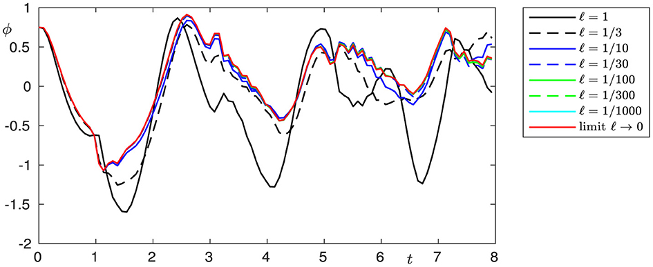
Figure 2. Transversal displacement of the beam, cross-section x = 2.

Figure 3

Figure 3. Transversal displacement of the beam, cross-section x = 6.

Figure 4

Figure 4. Shear angle variation of the beam, cross-section x = 2.

Figure 5

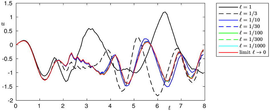
Figure 5. Shear angle variation of the beam, cross-section x = 6.

Figure 6

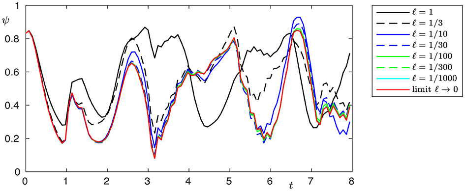
Figure 6. Longitudinal displacement of the beam, cross-section x = 2.

Figure 7

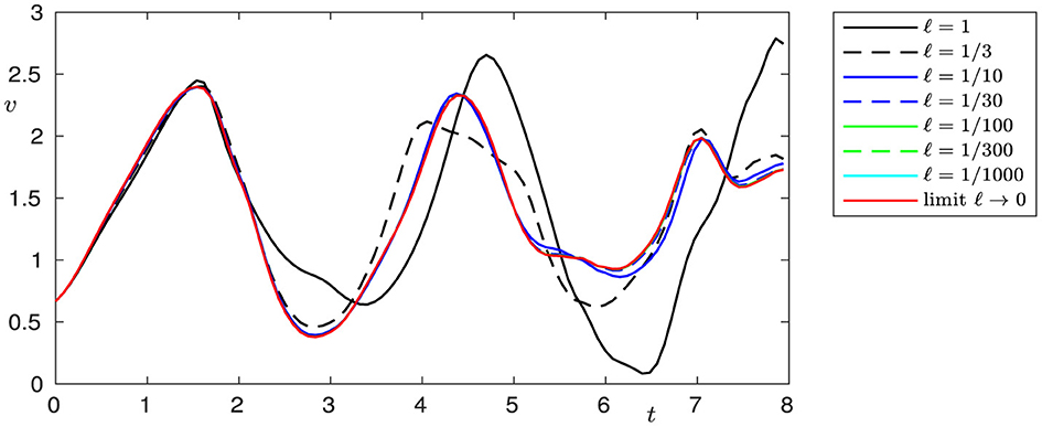
Figure 7. Longitudinal displacement of the beam, cross-section x = 6.

5.2 Singular limit k_i → ∞, l → 0

The singular limit for the straight Timoshenko beam (l = 0) as k_i → +∞ is the Euler–Bernoulli beam equation in Ref. [15, Ch. 4]. We have a similar result for the Bresse composite beam when k_i → ∞, and l → 0.

Theorem 5.3. Let the conditions of Theorem 3.4, (N6), and (D3) hold.

We also let the following assumptions be satisfied

$\begin{array}{c}({\phi }_0,u_0)\in \{{\phi }_0\in H^2(0,L_0),u_0\in H^2(L_0,L),{\phi }_0(0)=u_0(L)=0,\\ {\partial }_x{\varphi }_0(0)={\partial }_x{u}_0(L)=0,{\partial }_x{\phi }_0(L_0,t)={\partial }_x{u}_0(L_0,t)\};& (\mathrm{I1})\end{array}$

$\begin{array}{cc}{\psi }_0=-{\partial }_x{\phi }_0,v_0=-{\partial }_x{u}_0;& (\mathrm{I2})\end{array}$

$\begin{array}{l}({\phi }_1,u_1)\in \{{\phi }_1\in H^1(0,L_0),u_1\in H^1(L_0,L),{\phi }_1(0)=u_1(L)=0,\\ {\phi }_1(L_0,t)=u_1(L_0,t)\};& (\mathrm{I3})\end{array}$

$\begin{array}{cc}{\omega }_0=w_0=0;& (\mathrm{I4})\end{array}$

$\begin{array}{cc}{h}_1,h_2\in C^1({ℝ}^2);& (\mathrm{N6})\end{array}$

$\begin{array}{c}{r}_1\in L^{\infty }(0,T;H^1(0,L_0)),r_2\in L^{\infty }(0,T;H^1(L_0,L)),\\ r_1(L_0,t)=r_2(L_0,t)\text{ for allmost all }t>0.& (\mathrm{R3})\end{array}$

Let $k_j^{(n)}\to \infty$, l⁽ⁿ⁾ → 0 as n → ∞, and Φ⁽ⁿ⁾ be the solutions to (17)–(23) with the fixed $k_j^{(n)},l^{(n)}$ and the same initial data

$\begin{array}{c}\Phi (x,0)=({\phi }_0,{\psi }_0,{\omega }_0,u_0,v_0,w_0)(x),\\ {\Phi }_t(x,0)=({\phi }_1,{\psi }_1,{\omega }_1,u_1,v_1,w_1).\end{array}$

Then for every T > 0

$\begin{array}{l}{\Phi }^{(n)}\stackrel{*}{\rightharpoonup }(\phi ,\psi ,\omega ,u,v,w)\text{ in }{L}^{\infty }(0,T;H_d)\text{ as }n\to \infty ,\\ {\Phi }_t^{(n)}\stackrel{*}{\rightharpoonup }({\phi }_t,{\psi }_t,{\omega }_t,u_t,v_t,w_t)\text{ in }{L}^{\infty }(0,T;H_v)\text{ as }n\to \infty ,\end{array}$

where

• (φ, u) is the solution to

$\begin{array}{ll}\begin{array}{l}{\rho }_1{\phi }_{tt}-{\beta }_1{\phi }_{ttxx}+{\lambda }_1{\phi }_{xxxx}-{\gamma }^{\prime }(-{\phi }_{tx}){\phi }_{txx}+{\partial }_x{h}_1(\phi ,-{\phi }_x)\\ +f_1(\phi ,-{\phi }_x)=p_1(x,t)+{\partial }_x{r}_1(x,t),(x,t)\in (0,L_0)\times (0,T),\end{array}& (115)\end{array}$

$\begin{array}{ll}\begin{array}{l}{\rho }_2{u}_{tt}-{\beta }_2{u}_{ttxx}+{\lambda }_2{u}_{xxxx}+{\partial }_x{h}_2(u,-u_x)+f_2(u,-u_x)\\ =p_2(x,t)+{\partial }_x{r}_2(x,t),(x,t)\in (L_0,L)\times (0,T),\end{array}& (116)\end{array}$

$\begin{array}{cc}\phi (0,t)={\phi }_x(0,t)=0,u(L,t)=u_x(L,t)=0,& (117)\end{array}$

$\begin{array}{cc}\phi (L_0,t)=u(L_0,t),{\phi }_x(L_0,t)=u_x(L_0,t),& (118)\end{array}$

$\begin{array}{cc}{\lambda }_1{\phi }_{xx}(L_0,t)={\lambda }_2{u}_{xx}(L_0,t),& (119)\end{array}$

$\begin{array}{l}{\lambda }_1{\phi }_{xxx}(L_0,t)-{\beta }_1{\phi }_{ttx}(L_0,t)+h_1(\phi (L_0,t),\\ -{\phi }_x(L_0,t))+\gamma (-{\phi }_{tx}(L_0,t))=\\ {\lambda }_2{u}_{xxx}(L_0,t)-{\beta }_2{u}_{ttx}(L_0,t)+h_2(u(L_0,t),-u_x(L_0,t)),& (120)\end{array}$

with the initial conditions

$\begin{array}{c}(\phi ,u)(x,0)=({\phi }_0,u_0)(x),({\phi }_t,u_t)(x,0)=({\phi }_1,u_1)(x).\end{array}$

• ψ = −φ_x, v = −u_x;

• (ω, w) is the solution to

$\begin{array}{cc}{\rho }_1{\omega }_{tt}-{\sigma }_1{\omega }_{xx}+g_1(\omega )=q_1(x,t),(x,t)\in (0,L_0)\times (0,T),& (121)\end{array}$

$\begin{array}{cc}{\rho }_2{w}_{tt}-{\sigma }_2{w}_{xx}+g_2(w)=q_2(x,t),(x,t)\in (L_0,L)\times (0,T),& (122)\end{array}$

$\begin{array}{cc}\omega (0,t)=0,w(L,t)=0,& (123)\end{array}$

$\begin{array}{cc}{\sigma }_1{\omega }_x(L_0,t)={\sigma }_2{w}_x(L_0,t),\omega (L_0,t)=w(L_0,t)& (124)\end{array}$

with the initial conditions

$\begin{array}{c}(\omega ,w)(x,0)=(0,0),({\omega }_t,w_t)(x,0)=({\omega }_1,w_1)(x).\end{array}$

Proof. The proof uses the idea from Ref. [15, Ch. 4.3] and differs from it mainly in transmission conditions. We skip the details of the proof, which coincides with Ref. [15].

Energy inequality (25) implies (125)

$\begin{array}{ccc}{\partial }_t({\phi }^{(n)},{\psi }^{(n)},{\omega }^{(n)},u^{(n)},v^{(n)},w^{(n)})& \text{ bounded in }{L}^{\infty }(0,T;H_v),& (125)\end{array}$

$\begin{array}{ccc}{\psi }^{(n)}& \text{ bounded in }{L}^{\infty }(0,T;H^1(0,L_0)),& (126)\end{array}$

$\begin{array}{ccc}{v}^{(n)}& \text{ bounded in }{L}^{\infty }(0,T;H^1(L_0,L))& (127)\end{array}$

$\begin{array}{ccc}{\omega }_x^{(n)}-l^{(n)}{\phi }^{(n)}& \text{ bounded in }{L}^{\infty }(0,T;L_2(0,L_0)),& (128)\end{array}$

$\begin{array}{ccc}{w}_x^{(n)}-l^{(n)}{u}^{(n)}& \text{ bounded in }{L}^{\infty }(0,T;L_2(L_0,L)),& (129)\end{array}$

$\begin{array}{ccc}{k}_1^{(n)}({\phi }_x^{(n)}+{\psi }^{(n)}+l^{(n)}{\omega }^{(n)})& \text{ bounded in }{L}^{\infty }(0,T;L_2(0,L_0)),& (130)\end{array}$

$\begin{array}{ccc}{k}_2^{(n)}(u_x^{(n)}+v^{(n)}+l^{(n)}{w}^{(n)})& \text{ bounded in }{L}^{\infty }(0,T;L_2(L_0,L)),& (131)\end{array}$

Thus, we can extract subsequences that converge in corresponding spaces *-weak. Similarly to Ref. [15] we have

$\begin{array}{c}{\phi }_x^{(n)}+{\psi }^{(n)}+l^{(n)}{\omega }^{(n)}\stackrel{*}{\rightharpoonup }0\text{ in }{L}^{\infty }(0,T;L_2(0,L_0)),\end{array}$

therefore

$\begin{array}{c}{\phi }_x=-\psi .\end{array}$

Analogously,

$\begin{array}{c}{u}_x=-v.\end{array}$

Equations (126)–(131) imply

$\begin{array}{c}{\omega }^{(n)}\stackrel{*}{\rightharpoonup }\omega \text{ in }{L}^{\infty }(0,T;H^1(0,L_0)),\\ w^{(n)}\stackrel{*}{\rightharpoonup }w\text{ in }{L}^{\infty }(0,T;H^1(L_0,L)),& (132)\end{array}$

$\begin{array}{c}{\phi }^{(n)}\stackrel{*}{\rightharpoonup }\phi \text{ in }{L}^{\infty }(0,T;H^1(0,L_0)),\\ u^{(n)}\stackrel{*}{\rightharpoonup }u\text{ in }{L}^{\infty }(0,T;H^1(L_0,L)).& (133)\end{array}$

Thus, the Aubin's lemma gives that

$\begin{array}{cc}{\Phi }^{(n)}\to \Phi \text{ strongly in }C(0,T;{[H^{1-\epsilon }(0,L_0)]}^3\times {[H^{1-\epsilon }(L_0,L)]}^3)& (134)\end{array}$

for every ε > 0 and then

$\begin{array}{c}{\partial }_x{\phi }_0+{\psi }_0+l^{(n)}{\omega }_0\to 0\text{strongly in }{H}^{-\epsilon }(0,L_0),\end{array}$

This implies that

$\begin{array}{c}{\partial }_x{\phi }_0=-{\psi }_0,{\omega }_0=0.\end{array}$

Analogously,

$\begin{array}{c}{\partial }_x{u}_0=-v_0,w_0=0.\end{array}$

Let us take a test function of the form $B=({\beta }^1,-{\beta }_x^1,0,{\beta }^2,-{\beta }_x^2,0)\in F_T$ such that ${\beta }_x^1(L_0,t)={\beta }_x^2(L_0,t)$ for almost all t. Due to (132)–(134) and Lemma 5.2 we can pass to the limit in variational equality (24) as n → ∞. In the same way as in Ref. [15, Ch. 4.3] we obtain, that limiting functions φ, u are of higher regularity and satisfy the following variational equality

$\begin{array}{c}{\displaystyle \underset{0}{\overset{T}{\int }}}{\displaystyle \underset{0}{\overset{L_0}{\int }}}({\rho }_1{\phi }_t{\beta }_t^1-{\beta }_1{\phi }_{tx}{\beta }_{tx}^1)dxdt\\ +{\displaystyle \underset{0}{\overset{T}{\int }}}{\displaystyle \underset{L_0}{\overset{L}{\int }}}({\rho }_2{u}_t{\beta }_t^2-{\beta }_1{u}_{tx}{\beta }_{tx}^2)dxdt\\ -{\displaystyle \underset{0}{\overset{L_0}{\int }}}({\rho }_1({\phi }_t{\beta }_t^1)(x,0)-{\beta }_1({\phi }_{tx}{\beta }_{tx}^1)(x,0))dx\\ +{\displaystyle \underset{L_0}{\overset{L}{\int }}}({\rho }_2(u_t{\beta }_t^2)(x,0)-{\beta }_1(u_{tx}{\beta }_{tx}^2)(x,0))dx\\ +{\displaystyle \underset{0}{\overset{T}{\int }}}{\displaystyle \underset{0}{\overset{L_0}{\int }}}{\lambda }_1{\phi }_{xx}{\beta }_{xx}^{1}dxdt\\ +{\displaystyle \underset{0}{\overset{T}{\int }}}{\displaystyle \underset{L_0}{\overset{L}{\int }}}{\lambda }_2{u}_{xx}{\beta }_{xx}^{2}dxdt\\ -{\displaystyle \underset{0}{\overset{T}{\int }}}{\displaystyle \underset{0}{\overset{L_0}{\int }}}{\gamma }^{\prime }(-{\phi }_{xt}){\phi }_{txx}{\beta }^{1}dxdt\\ +{\displaystyle \underset{0}{\overset{T}{\int }}}{\displaystyle \underset{0}{\overset{L_0}{\int }}}(f_1(\phi ,-{\phi }_x){\beta }^1-h_1(\phi ,-{\phi }_x){\beta }_x^1)dxdt\\ +{\displaystyle \underset{0}{\overset{T}{\int }}}{\displaystyle \underset{L_0}{\overset{L}{\int }}}(f_2(u,-u_x){\beta }^2-h_2(u,-u_x){\beta }_x^2)dxdt\\ ={\displaystyle \underset{0}{\overset{T}{\int }}}{\displaystyle \underset{0}{\overset{L_0}{\int }}}(p_1{\beta }^1-r_1{\beta }_x^1)dxdt\\ +{\displaystyle \underset{0}{\overset{T}{\int }}}{\displaystyle \underset{L_0}{\overset{L}{\int }}}(p_2{\beta }^2-r_2{\beta }_x^2)dxdt.& (135)\end{array}$

Provided φ and u are smooth enough, we can integrate (135) by parts concerning x and t and obtain

$\begin{array}{c}{\displaystyle \underset{0}{\overset{T}{\int }}}{\displaystyle \underset{0}{\overset{L_0}{\int }}}({\rho }_1-{\beta }_1{\partial }_{xx}){\phi }_{tt}{\beta }^{1}dxdt+{\displaystyle \underset{0}{\overset{T}{\int }}}{\displaystyle \underset{L_0}{\overset{L}{\int }}}({\rho }_2-{\beta }_2{\partial }_{xx})u_{tt}{\beta }^{2}dxdt\\ +{\displaystyle \underset{0}{\overset{T}{\int }}}\left[{\beta }_1{\phi }_{ttx}(t,L_0)-{\beta }_2{u}_{ttx}(t,L_0)\right]{\beta }^1(t,L_0)dt\\ +{\displaystyle \underset{0}{\overset{T}{\int }}}{\displaystyle \underset{0}{\overset{L_0}{\int }}}{\lambda }_1{\phi }_{xxxx}{\beta }^{1}dxdt+{\displaystyle \underset{0}{\overset{T}{\int }}}{\displaystyle \underset{L_0}{\overset{L}{\int }}}{\lambda }_2{u}_{xxxx}{\beta }^{2}dxdt\\ +{\displaystyle \underset{0}{\overset{T}{\int }}}\left[{\lambda }_1{\phi }_{xx}-{\lambda }_2{u}_{xx}\right](t,L_0){\beta }_x^1(t,L_0)dt\\ -{\displaystyle \underset{0}{\overset{T}{\int }}}\left[{\lambda }_1{\phi }_{xxx}-{\lambda }_2{u}_{xxx}\right](t,L_0){\beta }^1(t,L_0)dt\\ -{\displaystyle \underset{0}{\overset{T}{\int }}}{\displaystyle \underset{0}{\overset{L_0}{\int }}}{\gamma }^{\prime }(-{\phi }_{xt}){\phi }_{xxt}{\beta }^{1}dxdt\\ -{\displaystyle \underset{0}{\overset{T}{\int }}}\gamma (-{\phi }_{xt}(L_0,t)){\beta }^1(L_0,t)\\ +{\displaystyle \underset{0}{\overset{T}{\int }}}{\displaystyle \underset{0}{\overset{L_0}{\int }}}(f_1(\phi ,-{\phi }_x)+{\partial }_x{h}_1(\phi ,-{\phi }_x)){\beta }^{1}dxdt\\ +{\displaystyle \underset{0}{\overset{T}{\int }}}{\displaystyle \underset{L_0}{\overset{L}{\int }}}(f_2(u,-u_x)+{\partial }_x{h}_2(u,-u_x)){\beta }^{2}dxdt\\ +{\displaystyle \underset{0}{\overset{T}{\int }}}(h_2(u(L_0,t),-u_x(L_0,T))-h_1(\phi (L_0,t),-{\phi }_x(L_0,T))){\beta }^1(L_0,t)dt\\ ={\displaystyle \underset{0}{\overset{T}{\int }}}{\displaystyle \underset{0}{\overset{L_0}{\int }}}(p_1+{\partial }_x{r}_1){\beta }^{1}dxdt+{\displaystyle \underset{0}{\overset{T}{\int }}}{\displaystyle \underset{L_0}{\overset{L}{\int }}}(p_2+{\partial }_x{r}_2){\beta }^{2}dxdt\\ +{\displaystyle \underset{0}{\overset{T}{\int }}}\left[r_2(t,L_0)-r_1(t,L_0)\right]{\beta }^1(t,L_0)dt.& (136)\end{array}$

Requiring all the terms containing ${\beta }^1(L_0,t)$, ${\beta }_x^1(L_0,t)$ to be zero, we get transmission conditions (119)–(116). Equations (115 and 116) are recovered from the variational equality (136). Problem (121)–(124) can be obtained in the same way.

We perform numerical modeling for the original problem with the initial parameters

$\begin{array}{c}{l}^{(1)}=1,k_1^{(1)}=4,k_2^{(1)}=1.\end{array}$

We model the simultaneous convergence l → 0 and k₁, and k₂ → ∞ in the following way: we divide l by the factor χ and multiply k₁, k₂ by the factor χ. Calculations were performed for the original problem with

$\begin{array}{c}\chi =1,\chi =3,\chi =10,\chi =30,\chi =100,\chi =300,\end{array}$

and the limiting problem (115)–(120). The other constants in the original problem are the same as in the previous subsection, and we change functions in the right-hand side (113, 114) as follows:

$r_1(x)=x+4,r_2(x)=2x.$

The nonlinear feedbacks are

$\begin{array}{ll}{f}_1(\phi ,\psi ,\omega )=4{\phi }^3-2\phi ,& f_2(u,v,w)=4u^3-8u,\\ h_1(\phi ,\psi ,\omega )=0,& h_2(u,v,w)=0,\\ g_1(\phi ,\psi ,\omega )=3\left|\omega \right|\omega ,& g_2(u,v,w)=6\left|w\right|w.\end{array}$

We use linear dissipation γ(s) = s, and we chose the following initial displacement and shear angle variation:

${\phi }_0(x)=-\frac{13}{640}{x}^4+\frac{6}{40}{x}^2-\frac{23}{40}{x}^2,$

$u_0(x)=\frac{41}{2160}{x}^4-\frac{68}{135}{x}^3+\frac{823}{180}{x}^2-\frac{439}{27}x+\frac{520}{27}.$

${\psi }_0(x)=-(-\frac{13}{160}{x}^3+\frac{27}{40}{x}^2-\frac{23}{20}x),$

$v_0(x)=-\left(\frac{41}{540}{x}^3-\frac{68}{45}{x}^2+\frac{823}{90}x-\frac{439}{27}\right).$

and set

$\begin{array}{c}{\omega }_0(x)=w_0(x)=0.\end{array}$

We choose the following initial velocities

${\phi }_1(x)=-\frac{1}{32}{x}^3+\frac{3}{16}{x}^2,u_1(x)=\frac{1}{108}{x}^3-\frac{7}{36}{x}^2+\frac{10}{9}x-\frac{25}{27},$

${\omega }_1(x)={\psi }_1(x)=\frac{3}{5}x,$

$w_1(x)=v_1(x)=-\frac{2}{5}x+4.$

The double limit case appeared to be more challenging from the point of view of numerics than the case l → 0. The numerical simulations of the coupled system in equations (1)–(7), including the interface conditions in (8)–(11), were done by a semi-discrete of the functions ϕ, ψ, ω, u, v, w with respect to the position x and by using an explicit scheme for the time integration. That allows the choice of discretized values at grid points near the interface in a separate step so that they obey the transmission conditions. It was necessary to solve a nonlinear system of equations for the six functions at three grid points (at the interface, and left and right of the interface) in each time step. Any attempt to use a fully implicit numerical scheme led to extremely time-expensive computations due to the large nonlinear system's overall discretized values which were to be solved in each time step. On the other hand, increasing k₁ and k₂ increases the stiffness of the system of ordinary differential equations, which results from the semidiscretization, and the CFL conditions require small time steps; otherwise, numerical oscillations occur. Figures 8–13 present smoothed numerical solutions, which were particularly necessary for large factors χ, e.g., χ = 300. When the parameters k₁ and k₂ are large, the material of the beam gets stiff, and so does the discretized system of differential equations. Nevertheless, the oscillations are still noticeable in the graph. By the way, the observation that the factor χ cannot be arbitrarily enlarged underlines the importance of having the limit problem for χ → ∞ in (1)-(15).

Figure 8

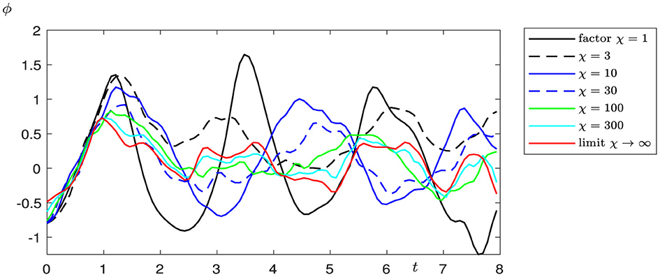
Figure 8. Transversal displacement of the beam, cross-section x = 2.

Figure 9

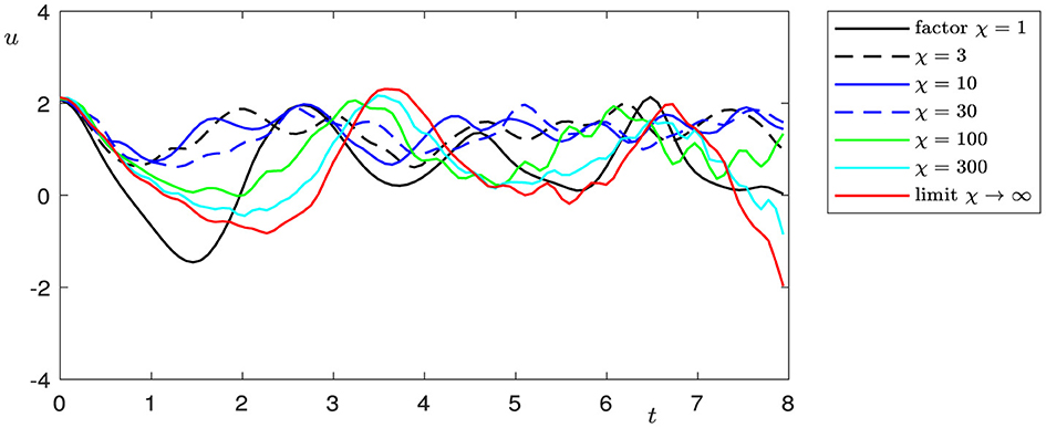
Figure 9. Transversal displacement of the beam, cross-section x = 6.

Figure 10

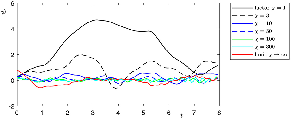
Figure 10. Shear angle variation of the beam, cross-section x = 2.

Figure 11

Figure 11. Shear angle variation of the beam, cross-section x = 6.

Figure 12

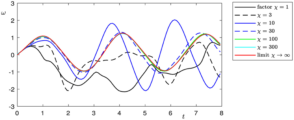
Figure 12. Longitudinal displacement of the beam, cross-section x = 2.

Figure 13

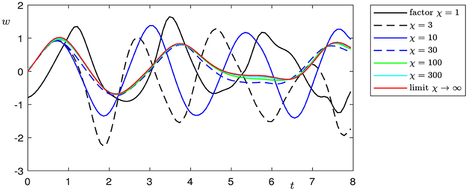
Figure 13. Longitudinal displacement of the beam, cross-section x = 6.

6 Discussion

The classical Kirchhoff model of elasticity is based on the hypothesis that the shear angle ψ can be represented as ψ = −∂_xφ, where ϕ is the transverse displacement of the beam. In this case, the beam is initially straight and nonshearable. The Bresse model describes the dynamics of an initially curved beam and takes into consideration shear effects (for details, see, e.g., Ref. [2]). In real-world applications, it is important to investigate networks of elastic objects with different elastic properties and contact conditions, such as spacecraft structures, trusses, robot arms, antennae, etc. In the present study, we evaluate the dynamics of two Bresse beams with rigid contact and, moreover, show that if the curvature l tends to zero, solutions to the Bresse transmission problem lean to be the solutions of two problems. The longitudinal displacements in this case incline to be the solutions to a transmission problem for a wave equation, and the transversal displacements and shear angles be the to solutions to the Timoshenko problem, describing the dynamics of a straight shearable beam. In the case of a double limit, if curvature l tends to zero and shear moduli k₁, and k₂ tend to infinity, the longitudinal displacements, in this case, tend to be the solutions of a transmission problem for a wave equation, and the transversal displacements to solutions of a transmission Kirchhoff problem with rotational inertia. We illustrate these effects by means of numerical modeling. These results show that in cases of small initial curvature and large shear moduli, shear effects can be neglected and the dynamics can be described by the well-known Kirchhoff model. Figures show that the speed of convergence to the limit model in the case of a single limit l → 0 is higher than in the case of a double limit l → 0, k_i → ∞, when not only the geometric configuration but also the elastic properties of the beam change.

There are many studies devoted to long-time behavior of linear homogeneous Bresse beams (with various boundary conditions and dissipation natures). If damping is present in all three equations, it appears to be sufficient for the exponential stability of the system without additional assumptions on the parameters of the problems (see, e.g., Ref. [16–18]).

The situation is different if we have a dissipation of any kind in two or one equation only. First of all, it matters in which equations the dissipation acts. There are results on the Timoshenko beams (see Ref. [19]) and the Bresse beams (see Ref. [20]) showing that damping in only one of the equations does not guarantee the exponential stability of the whole system. It seems that for the Bresse system, the presence of dissipation in the shear angle equation is necessary for stability of any kind. To get exponential stability, one needs additional assumptions on the coefficients of the problem, usually the equality of the propagation speeds:

$\begin{array}{c}{k}_1={\sigma }_1,\frac{{\rho }_1}{k_1}=\frac{{\beta }_1}{{\lambda }_1}\end{array}$

Otherwise, only polynomial (non-uniform) stability holds (see e.g., Ref. [21] for mechanical dissipation and Ref. [20] for thermal dissipation). In Ref. [22] analogous results are established in the case of nonlinear damping.

If dissipation is present in all three equations of the Bresse system, corresponding problems with nonlinear source forces of a local nature possess global attractors under the standard assumptions for nonlinear terms (see e.g., [4]). Otherwise, nonlinear source forces create technical difficulties and may cause instability in the system. To the best of our knowledge, there is no literature on such cases.

The damping force is a function of the system's velocity. In the linear case, it is standard linear viscous damping; however, in some mechanical systems, for instance, nonlinear suspension and isolation systems (see e.g., Ref. [23] Section 2d), the damping force can be nonlinear. Therefore, we consider a general nonlinear damping term and find assumptions under which the problem is well-posed and possesses a compact global attractor. In this case, linear damping is a particular case of the damping considered.

The presence of nonlinear feedback complicates the structure the of attractors. The homogeneous problem without nonlinear feedbacks is exponentially stable, and its trajectories stabilize to zero for infinite time. Nonlinear problems usually have more complex limiting regimes. In this case, the attractor consists of full trajectories stabilizing the set of stationary points, which can consist of multiple points.

In this study, we investigate a transmission problem for the Bresse system.

Transmission problems for various equation types have already had some history of investigation. One can find many research concerning their well-posedness, long-time behavior, and other aspects (see e.g., Ref. [24] for a nonlinear thermoelastic/isothermal plate, Ref. [25] for the Kirchhoff/Timoshenko beam, and Ref. [26] for the full von Karman beam). Problems with localized damping are close to transmission problems. In recent years a number of such problems for the Bresse beams have been studied, e.g., Ref. [4, 22]. To prove the existence of attractors in this case, a unique continuation property is an important tool, as well as the frequency method.

The only interpretation we know on a transmission problem for the Bresse system is Ref. [27]. The beam in this work consists of thermoelastic (damped) and elastic (undamped) parts, both purely linear. Despite the presence of dissipation in all three equations for the damped part, the corresponding semigroup is not exponentially stable for any set of parameters but only polynomially (non-uniformly) stable. In contrast to Ref. [27], we consider mechanical damping only in the equation for the shear angle for the damped part. However, we can establish exponential stability for the linear problem and the existence of an attractor for the nonlinear one under restrictions on the coefficients in the damped part only. The assumption on the nonlinearities can be simplified in the 1D case (cf. e.g., Ref. [28]).

Data availability statement

The original contributions presented in the study are included in the article/supplementary material, further inquiries can be directed to the corresponding author.

Author contributions

TF: Methodology, Investigation, Formal analysis, Data curation, Conceptualization, Writing – review & editing, Writing – original draft. DL: Writing – review & editing, Writing – original draft, Visualization, Software, Methodology, Investigation, Data curation, Conceptualization. IR: Formal analysis, Methodology, Investigation, Data curation, Conceptualization, Writing – review & editing, Writing – original draft.

Funding

The author(s) declare financial support was received for the research, authorship, and/or publication of this article. The research was supported by the Volkswagen Foundation project “From Modeling and Analysis to Approximation”. TF and IR were also successively supported by the Volkswagen Foundation project “Dynamic Phenomena in Elasticity Problems” at Humboldt-Universität zu Berlin, Funding for Refugee Scholars and Scientists from Ukraine.

Conflict of interest

The authors declare that the research was conducted in the absence of any commercial or financial relationships that could be construed as a potential conflict of interest.

Publisher's note

All claims expressed in this article are solely those of the authors and do not necessarily represent those of their affiliated organizations, or those of the publisher, the editors and the reviewers. Any product that may be evaluated in this article, or claim that may be made by its manufacturer, is not guaranteed or endorsed by the publisher.

References

1. Bresse JAC. Cours de Mechanique Appliquee. Paris: Mallet Bachelier. (1859).

Google Scholar

2. Lagnese JE, Leugering G, Schmidt EJPG. Modeling, Analysis and Control of Dynamic Elastic Multi-Link Structures. Boston: Birkhäuser. (1994).

Google Scholar

3. Triggiani R, Yao PF. Carleman estimates with no lower-order terms for general Riemann wave equations. Global uniqueness and observability in one shot. Appl Math Optim. (2002) 46:331–75. doi: 10.1007/s00245-002-0751-5

Crossref Full Text | Google Scholar

4. Ma TF, Monteiro RN. Singular limit and long-time dynamics of Bresse systems. SIAM J Mathematical Analysis. (2017) 49:2468–95. doi: 10.1137/15M1039894

Crossref Full Text | Google Scholar

5. Liu W, Williams GH. Exact Controllability for problems of transmission of the plate equation with lower-order terms. Quart Appl Math. (2000) 58:37–68. doi: 10.1090/qam/1738557

Crossref Full Text | Google Scholar

6. Chueshov I, Eller M, Lasiecka I. On the attractor for a semilinear wave equation with critical exponent and nonlinear boundary. dissipation. Commun Partial Differ Equations. (2002) 27:1901–51. doi: 10.1081/PDE-120016132

Crossref Full Text | Google Scholar

7. Barbu V. Nonlinear Semigroups and Differential Equations in Banach Spaces. Nordhoff Pl: Nordhof. (1976).

PubMed Abstract | Google Scholar

8. Chueshov I, Lasiecka I. Long-time dynamics of von Karman semi-flows with non-linear boundary/interior damping. J Differ Equations. (2007) 233:42–86. doi: 10.1016/j.jde.2006.09.019

Crossref Full Text | Google Scholar

9. Chueshov I. Introduction to the Theory of Infinite-Dimensional Dissipative Systems. Kharkiv: Acta. (2002).

Google Scholar

10. Chueshov I, Fastovska T, Ryzhkova I. Quasistability method in study of asymptotical behaviour of dynamical systems. J Math Phys Anal Geom. (2019) 15:448–501. doi: 10.15407/mag15.04.448

Crossref Full Text | Google Scholar

11. Chueshov I, Lasiecka I. Long-Time Behavior of Second Order Evolution Equations with Nonlinear Damping. Providence, RI: Memoirs of AMS 912, AMS. (2008).

Google Scholar

12. Kanwal RP. Generalized Functions. Theory and Applications. Basel: Birkhäuser. (2004). doi: 10.1007/978-0-8176-8174-6

Crossref Full Text | Google Scholar

13. Lasiecka I, Triggiani R. Regularity of hyperbolic equations under L²(0, T; L²(Γ))-Dirichlet boundary terms. Appl Math Optim. (1983) 10:275–86. doi: 10.1007/BF01448390

Crossref Full Text | Google Scholar

14. Khanmamedov A. Global attractors for von Karman equations with nonlinear dissipation. J Math Anal Appl. (2016) 318:92–101. doi: 10.1016/j.jmaa.2005.05.031

Crossref Full Text | Google Scholar

15. Lagnese JE. Boundary Stabilization of Thin Plates. Philadelphia, PA: SIAM. (1989). doi: 10.1137/1.9781611970821

Crossref Full Text | Google Scholar

16. da S Almeida Junior D, Santos ML. Numerical exponential decay to dissipative Bresse system. J Appl Math. (2010) 848620:17. doi: 10.1155/2010/848620

Crossref Full Text | Google Scholar

17. Mukiawa SE, Enuy CD, Apalara TA. A new stability result for a thermoelastic Bresse system with viscoelastic damping. J Inequal Appl. (2021) 137:1–26. doi: 10.1186/s13660-021-02673-0

Crossref Full Text | Google Scholar

18. Mukiawa E. A new optimal and general stability result for a thermoelastic Bresse system with Maxwell-Cattaneo heat conduction. Results Appl Math. (2021) 10:1–20. doi: 10.1016/j.rinam.2021.100152

Crossref Full Text | Google Scholar

19. Rivera JEM, Racke R. Mildly dissipative nonlinear Timoshenko systems—global existence and exponential stability. J Math Anal Appl. (2002) 276:248–78. doi: 10.1016/S0022-247X(02)00436-5

Crossref Full Text | Google Scholar

20. Dell'Oro F. Asymptotic stability of thermoelastic systems of Bresse type. J Differ Equations. (2015) 258:3902–27. doi: 10.1016/j.jde.2015.01.025

Crossref Full Text | Google Scholar

21. Alabau-Boussouira F, Munoz-Rivera JE, da Almeida Junior D. Stability to weak dissipative Bresse system. J Math Anal Appl. (2011) 374:481–98. doi: 10.1016/j.jmaa.2010.07.046

Crossref Full Text | Google Scholar

22. Charles W, Soriano JA, Nascimento FAF, Rodrigues JH. Decay rates for Bresse system with arbitrary nonlinear localized damping. J Differ Equations. (2013) 255:2267–90. doi: 10.1016/j.jde.2013.06.014

Crossref Full Text | Google Scholar

23. Elliott SJ, Tehrani MG, Langley RS. Nonlinear damping and quasi-linear modelling. Phil Trans R Soc A. (2015) 215:20140402. doi: 10.1098/rsta.2014.0402

PubMed Abstract | Crossref Full Text | Google Scholar

24. Potomkin M. A nonlinear transmission problem for a compound plate with thermoelastic part. Math Meth Appl Sci. (2012) 35:530–46. doi: 10.1002/mma.1589

Crossref Full Text | Google Scholar

25. Fastovska T. Decay rates for Kirchhoff-Timoshenko transmission problems. Commun Pure Appl Anal. (2013) 12:2645–67. doi: 10.3934/cpaa.2013.12.2645

Crossref Full Text | Google Scholar

26. Fastovska T. Global attractors for a full von Karman beam transmission problem. Commun Pure Appl Anal. (2023) 22:1120–58. doi: 10.3934/cpaa.2023022

Crossref Full Text | Google Scholar

27. Youssef W. Asymptotic behavior of the transmission problem of the Bresse beam in thermoelasticity. Z Angew Math Phys. (2022) 73:7. doi: 10.1007/s00033-022-01797-7

Crossref Full Text | Google Scholar

28. Fastovska T. Attractor for a composite system of nonlinear wave and thermoelastic plate equations. Visnyk Kharkiv. Nat Univer. (2014) 70:4–35.

Google Scholar