 Cristian Carvajal-Muquillaza
 Ronald Manríquez
- Laboratorio de Investigación Lab[e]saM, Departamento de Matemática, Física y Computación, Universidad de Playa Ancha, Valparaíso, Chile
Introduction: This article introduces a new family of weighted mixture distributions, referred to as θ-WM. The θ-WM family is generated by combining two distributions weighted by a parameter θ, offering notable flexibility to model a wide range of complex phenomena. A special case study of the θ-weighted mixture distribution of Weibull-Lomax (θ-WMWLx) is included, resulting from the combination of Weibull and Lomax distributions.
Methods: The research thoroughly examines the reliability and statistical properties of the θ-WMWLx distribution. Key aspects such as stochastic dominance, survival and hazard functions, mean residual life, and moments are addressed. The maximum likelihood method is used to estimate unknown parameters.
Results: The research findings show that the θ-WMWLx distribution provides a superior fit compared to competing distributions. The analyses are validated using three real datasets, demonstrating the effectiveness of the proposed distribution.
Discussion: The θ-WMWLx distribution stands out for its ability to model complex phenomena with high precision. Validation with real data confirms that the proposed distribution offers a better fit than existing distributions, highlighting its utility and applicability in various statistical analysis contexts.
1 Introduction
In scientific research, distribution models constitute conceptual frameworks to comprehend complex phenomena. These models span from the intricacies of climate change and pandemic spread to understanding the dynamics of economic indicators or the lifespan of cellular organisms. Granting these models, significant flexibility is essential to align them with the inherent complexities of the studied phenomena. The establishment of new parameters into distribution models gives them greater adaptability to diverse circumstances.
The study of generalized probability distributions begins with the famous study on Pearson's systems of continuous distributions, in which each probability density function satisfies a differential equation with four parameters on which the shape of the function depends (see Pearson [1]). In Amoroso [2], the generalization of the beta distribution to better fit certain income rates is discussed. Following Pearson's ideas, Burr [3] presents a system of continuous distributions that also satisfy a differential equation. Later, Johnson [4] proposed a system to generate distributions using the normalization transformation with four parameters: two of shape, one of scale, and one of location.
A pivotal contribution in this field emerged from the study of Marshall and Olkin [5], and their method defines a new survival function as follows:
where , and represents the survival function of a random variable X.
From Equation (1), extensive research has led to new distribution families such as the Marshall-Olkin generalized exponential linear distribution proposed by Okasha and Kayid [6], the extended uniform distribution of Marshall-Olkin by Jose and Krishna [7], the Marshall-Olkin Topp-Leone half-logistic-G distribution by Sengweni et al. [8], the generalized Marshall-Olkin transmuted-G family in Handiquea et al. [9] that to extend the transmuted family proposed in Shaw and Buckley [10], and the Marshall-Olkin-Weibull-H family applied to COVID-19 data (see Afify et al. [11]). Based on incorporating parameters into a reference distribution, this approach has proven effective in fostering flexibility into new distribution families [12].
Another strategy for creating new distribution families involves functional transformations. For instance, Souza et al. [13] introduced the Sin-G family generated by the sine function. In addition, Shama et al. [14] proposed the Modified Generalized-G family, a flexible distribution built on power-exponential transformations. Their theoretical approach is as follows: let Ḡ be a survival function of an absolutely continuous distribution with support (0, 1), and H be a decreasing continuous function such that H(x)∈[0, 1] and . Then, the following function is a valid continuous distribution function:
Shama et al. chose G as the survival function of the T2ExG family defined with a certain generic baseline distribution and H as a decreasing exponential function compound with a possible other baseline distribution.
There is extensive literature associated with the generalization and/or obtaining of families of distributions that contemplate different techniques and strategies (see, for instance, Nadarajah and Kotz [15], Eugene et al. [16], Cordeiro and de Castro [17], Mahdavi and Kundu [18], and Iriarte et al. [19]).
This study aims to construct a new distribution family called θ-Weighted Mixture distribution (θ-WM) based on the approach of Equation (2) by incorporating a parameter θ∈[0, 1] and considering H as a survival function and, thus, to expand de proposal of Shama et al. [14]. This general family is established as a flexible and adaptable framework for modeling diverse phenomena; it allows a gradual and flexible transition between G and H distributions through the weighting parameter θ, addressing a wider range of problems that require more accurate modeling. Specifically, we deal with a particular case within the θ-WM family, denoted by θ-WMWLx, composed of the Weibull and Lomax distributions. We study the fundamental reliability components associated with the θ-WMWLx distribution, along with its basic statistical properties such as survival and hazard functions, mean residual life, mean inactivity time, useful expansions, quantile function, Renyi entropy, moments, order statistics, and estimation methods. Furthermore, we present two real datasets to compare the behavior of the proposed distribution with four other models.
The θ-WM family has desirable properties, justified as follows: (i) The specific submodels of the θ-WM family, such as θ-WMEW and θ-WMWLx, can represent crucial hazard rate (hr) shapes, including increasing, decreasing, J-shape, and reversed J-shape; (ii) in addition, the densities of its submodels encompass reversed J-shaped, right-skewed, symmetric, left-skewed, and decreasing–increasing–decreasing patterns; (iii) the specific θ-WMWLx model provides a better fit compared to other generalized models using the same baseline distribution, as demonstrated in the case of the Lomax-exponential distribution (LED) and the exponentiated Kumaraswamy Inverse Weibull (EKIW) distribution.
The document is structured as follows: Section 2 introduces the θ-Weighted Mixture distribution family (θ-WM) based on Equation (2). In Section 3, we study the θ-WMWLx distribution as part of the θ-WM family. Section 4 encompasses a comprehensive reliability analysis, including a detailed exploration of the fundamental statistical properties of the θ-WMWLx distribution.
In Section 5, a simulation study is incorporated to evaluate the performance of maximum likelihood estimators (MLE), least squares estimators (LSE), and weighted least squares estimators (WLSE) across various sample sizes and parameter configurations. Finally, two real-world applications are presented to demonstrate the behavior of the proposed distribution compared to four other models, and the conclusion drawn from the study is summarized in Section 6.
2 The θ-Weighted Mixture distribution family (θ-WM)
In this section, we introduce the definition of the θ-Weighted Mixture distribution family (θ-WM), based on Equation (2). In addition, we show two distribution models from this proposed family as illustrative examples.
Definition 1. Let G(x|η) and Ψ(x|ξ) be two absolutely continuous baseline distribution functions, where Ḡ(x|η) and represent their respective survival functions (SF). Then, for θ∈[0, 1], the corresponding cumulative distribution function (CDF) and probability density function (PDF) for the θ-WM distribution family are obtained as follows:
and
where g and ψ are the PDFs of the distributions G and Ψ, respectively.
Remark 1. From the definition 1, we have:
1. The parameter θ determines the weighting between the survival functions Ḡ and in the formation of the combined distribution.
2. If θ = 0, then F0(x|η, ξ) = G(x|η).
3. If θ = 1, then F1(x|η, ξ) = Ψ(x|ξ).
4. If G(x|Φ) = Ψ(x|Φ), then Fθ(x|Φ) = G(x|Φ).
2.1 Some models based on the θ-WM distribution family
In this subsection, two models are shown using Equations (3, 4) to determine both the cumulative distribution function and probability density function of the θ-WM distribution family for each of these models.
Figures 1–3 show the HRFs of the submodels in the θ-WM family. The flexibility of these graphs can be observed, displaying increasing shapes, J-shapes, unimodal, and asymmetric forms. Similarly, the densities of these submodels provide great flexibility in their shapes, which can exhibit left-skewed, bimodal, right-skewed, unimodal, symmetrical, and J-shaped forms, as illustrated in Figures 1–3.
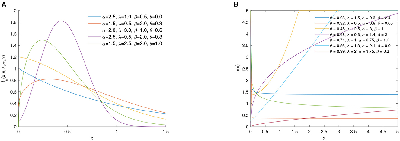
Figure 1. (A) PDF of θ-WMEW. (B) HRF of θ-WMEW.
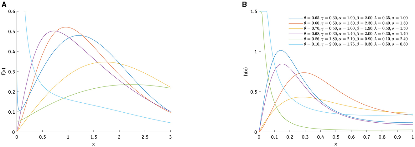
Figure 2. (A) PDF of θ-WMPLxR. (B) HRF of θ-WMPLxR.

Figure 3. (A) PDF of θ-WMWLx distribution. (B) HRF of θ-WMWLx distribution.
2.1.1 The θ-WMEW distribution
We define the θ-WMEW distribution by taking the exponential and Weibull distributions as baseline distributions in the θ-WM distribution family.
Suppose X1 is a random variable that follows an exponential distribution with parameter λ. Then, the CDF and PDF of X1 are defined by G(x|λ) = 1−e−λx and g(x|λ) = λe−λx, respectively, and the random variable X2 follows a Weibull distribution with shape parameter α and scale parameter β. The CDF and PDF of X2 are expressed as Ψ(x|α, β) = 1−e−(βx)α and ψ(x|α, β) = αβ(βx)α−1e−(βx)α, respectively. Consequently, the CDF and PDF of the θ-WMEW distribution are given by
and
where θ represents a parameter that weights the characteristics of the exponential and Weibull distributions. Figure 1 shows the graph of PDF and hazard rate function HRF for different parameters.
2.1.2 The θ-WMPLxR distribution
The θ-WMPLxR distribution corresponds to the composition of the Marshall-Olkin power Lomax and Rayleigh distributions. Then, the CDF and PDF of the θ-WMPLxR distribution are expressed as follows:
and
Figure 2 shows the graph of the PDF and HRF of the θ-WMPLxR distribution for different parameter values.
3 θ-Weighted Mixture Weibull-Lomax distribution (θ-WMWLx)
Within the framework of the family of θ-weighted mixture distributions (θ-WM) emerges the θ-weighted mixture Weibull-Lomax distribution (θ-WMWLx). Based on the strategic fusion of the Weibull and Lomax distributions, this theoretical expansion provides a powerful and adaptable tool for modeling phenomena with diverse and complementary properties.
The specific choice of the Weibull and Lomax distributions is not arbitrary; rather, it is grounded in their inherent characteristics that make them exceptionally suitable for modeling different contexts and phenomena. The Weibull distribution is recognized for its versatility in modeling product lifetimes, reliability phenomena, and time to failure, while the Lomax distribution, known as the two-parameter Pareto distribution, stands out for its ability to describe phenomena with heavy tails and long-tailed distributions. For more details, refer to the studies Tahir et al. [20], Afify et al. [21], Hassan and Abd-Allah [22], Ijaz et al. [23], and Alzaghal et al. [24].
The main distinction of the θ-WMWLx lies in its ability to encapsulate both the shape of the Weibull distribution, with its flexibility in modeling different behaviors, and the heavy-tailed characteristics of the Lomax distribution. This fusion provides a powerful and adaptable statistical framework to describe a wide range of phenomena, from data exhibiting reliability trends and lifetimes to those showing extreme behaviors and long tails.
Let Ḡ(x|λ, k) and be the survival functions of the Weibull and Lomax distributions, respectively, that is Ḡ(x|λ, k) = e−(λx)k and . Then, according to Definition 1, and for 0 ≤ θ ≤ 1, the CDF and PDF for θ-WMWLx are defined by
and
respectively.
Figure 3 shows the graph of the PDF and HRF of the θ-WMWLx distribution for a combination of λ, k, β, α, and θ parameters.
It is evident that the densities of the θ-WMWLx distribution (Equation 6) exhibit diverse shapes, ranging from symmetric to asymmetric, with skewness, inverted J-shaped, and unimodal distributions.
These graphs illustrate how the PDF may show various behaviors for θ and k values. For instance, when θ = 0 and 0 < k ≤ 1, the PDF decreases. However, if θ = 0 and k>1, the PDF increases when X < 1/k((k−1)/k)1/k and decreases when X < 1/k((k−1)/k)1/k. Finally, for θ = 1, the PDF always exhibits a decreasing trend.
Proposition 1 shows a stochastic order connection between Ḡ(x|λ, k) and Fθ(x|θ, λ, k, α, β).
Proposition 1. If Fθ(x|θ, λ, k, α, β) is defined as in Equation (5) and , then Fθ(x|θ, λ, k, α, β) exhibits first-order stochastic dominance over , that is,
Proof. To prove first-order stochastic dominance, we need to prove that
Subtracting the CDF functions yields
We know that e−(1−θ)(λx)k>0 for all x, so if (1−(1+βx)−θα)≥0 for all x>0, stochastic dominance holds.
The expression (1−(1+βx)−θα)≥0 is satisfied whenever (1+βx)−θα ≤ 1, which is factual since (1+βx)−θα is a decreasing function in x and for θ, α>0. This proves the result. ⃣
Figure 4 clearly shows the first-order stochastic dominance of Fθ(x) over
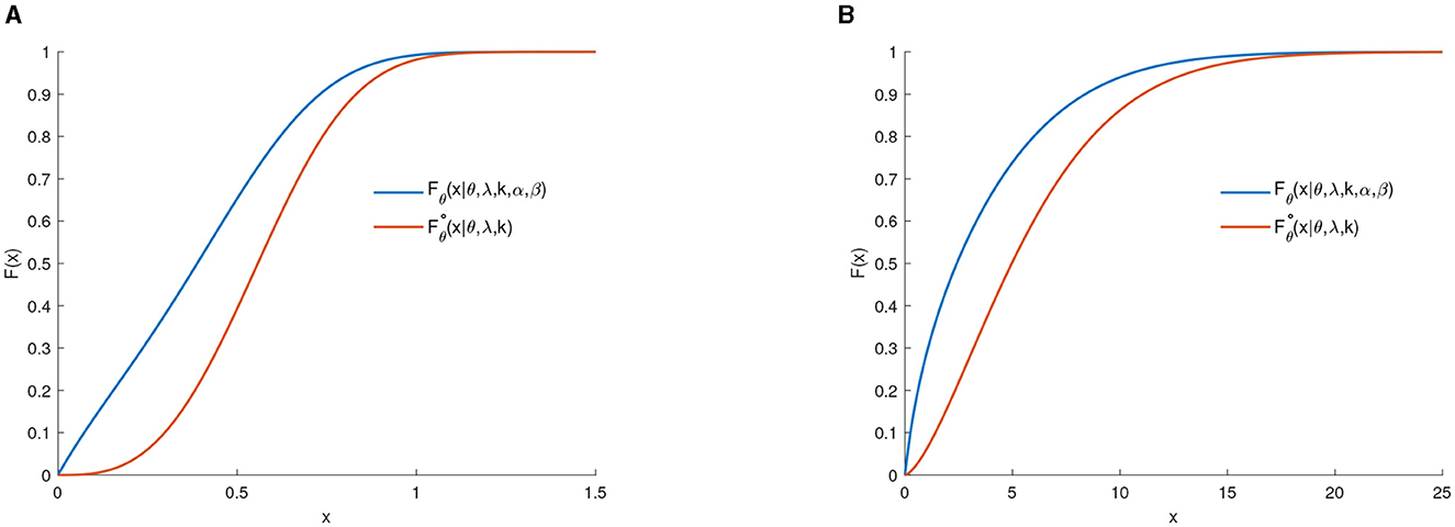
Figure 4. (A) CDF F0.5(x) and . (B) CDF F0.3(x) and .
4 Reliability elements and statistical properties of the θ-WMWLx distribution
In this section, we study the fundamental reliability components associated with the θ-WMWLx distribution, along with its basic statistical properties such as survival and hazard functions, mean residual life, mean inactivity time, useful expansions, quantile function, Renyi entropy, moments, order statistics, and estimation methods.
4.1 Survival and hazard functions
In survival analysis, one of the most important functions is the survival function, defined as the probability that an individual will survive beyond time x, as stated by Kartsonaki [25]. It is expressed as
Therefore, if X follows a θ-WMWLx (θ, λ, k, α, β) distribution, then the SF is represented by the equation:
This equation describes the probability of an individual's continued survival beyond time x. The hazard function, also known as the failure rate or hazard function, represents a component's instantaneous probability of failure, assuming failure has not occurred before time x (see Baredar et al. [26]). On the other hand, the reversed hazard rate is defined as the ratio between the probability density function and its distribution function (see Kayid et al. [27]). Therefore, if X follows a θ-WMWLx (θ, λ, k, α, β) distribution, the hazard function and the reversed hazard rate are expressed as
and
4.2 Mean residual life
The mean residual life (MRL) represents the anticipated added duration once a component has endured up to a time t. The MRL is crucial for reliability and survival analysis and characterizes the aging mechanism. It has been established that the MRL exclusively defines the distribution function, encapsulating all model-relevant details (see Alshangiti et al. [28]). If the random variable X represents the life of a component, then the MRL is given by
where is the survival function.
The MRL function of a lifetime random variable X with θ-WMWLx (θ, λ, k, α, β) distribution is given by
4.3 Mean inactivity time
The mean inactivity time (MIT) function is a reliability measure with applications in many disciplines, such as reliability theory, survival analysis, and actuarial studies. The MIT allows describing the time elapsed since a failure occurred. Let X be a lifetime random variable with distribution function F. The MIT function of X is defined by
The MIT function of a lifetime random variable X with θ-WMWLx (θ, λ, k, α, β) distribution is given by
4.4 Useful expansions
In this subsection, we provide an infinite mixture representation of the probability density function corresponding to the θ-WMWLx distribution, which will be used in some subsequent calculations.
It is well known that the exponential series expansion is given by
By applying Equation (9) to the PDF of θ-WMWLx, we obtain
where
4.5 Quantile function
The quantile function is obtained by solving:
where Q(·) is the CDF of θ-WMWLx (θ, λ, k, α, β) distribution. In this case, the quantile function is the solution of the non-linear equation:
By setting u = 0.5 in Equation (11), we can obtain the median (Me) of the θ-WMWLx distribution. Furthermore, the lower and higher quartiles can be obtained by setting u = 0.25 and u = 0.75, respectively.
Table 1 shows the quantiles Q1, Me, and Q3 for different values of the weighting parameter θ. These values were obtained using the root-finding method, specifically implemented computationally through the uniroot() function in R software version 4.3.3. The uniroot() function is used to find the roots of non-linear equations, and in this context, it was applied to solve an equation that models the relationship between the quantiles and the parameter θ.

Table 1. First quartile, median, and third quartile of θ-WMWLx distribution.
4.6 Rényi entropy
The entropy of a random variable X is a measure of the uncertain variation. The Rényi entropy is defined by
where
Let X~ θ-WMWLx (θ, λ, k, α, β). The corresponding Renyi entropy is obtained as
Table 2 shows the Renyi entropy for θ-WMWLx with δ = 2, α = 0.5, β = 1, λ = 0.3, k = 2, and different choices of parameter θ.
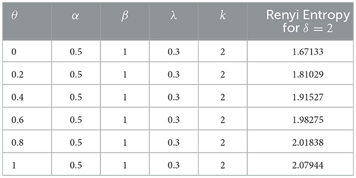
Table 2. Renyi entropy of θ-WMWLx.
For the calculation of Renyi entropy, the numerical integration method based on the integral() function in MATLAB version R2024a was used (see Algorithm 1).
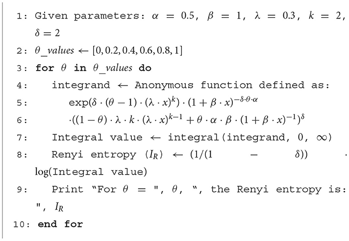
Algorithm 1. Pseudocode to calculate Renyi entropy for given parameters.
4.7 Moments
Moments in statistical analysis are essential measures that describe diverse probability distribution characteristics. They provide insights into the shape, center, spread, and other important features of the distribution. Specifically, moments help to quantify properties such as mean, variance, skewness, and kurtosis.
Theorem 2. If X~ θ-WMWLx (θ, λ, k, α, β), then the rth moment of X (for r < α, when θ = 1) is obtained by
where and is the Beta function.
Proof. We know that
Substituting Equation (10) into Equation (12) yields
If u = βx, then du = βdx, hence
Again, if , then , hence
⃣
From the above, the mean of X is given by . To determine the variance of X, we use the Koenig-Huygens formula, that is to say, Var(X) = E(X2)−[E(X)]2.
The r-th central moment is given by
By using Equation (13), we can obtain the skewness and kurtosis of X as follows:
Table 3 shows different moments of X for specific parameter combinations. MATLAB version R2024a was employed for their computation.
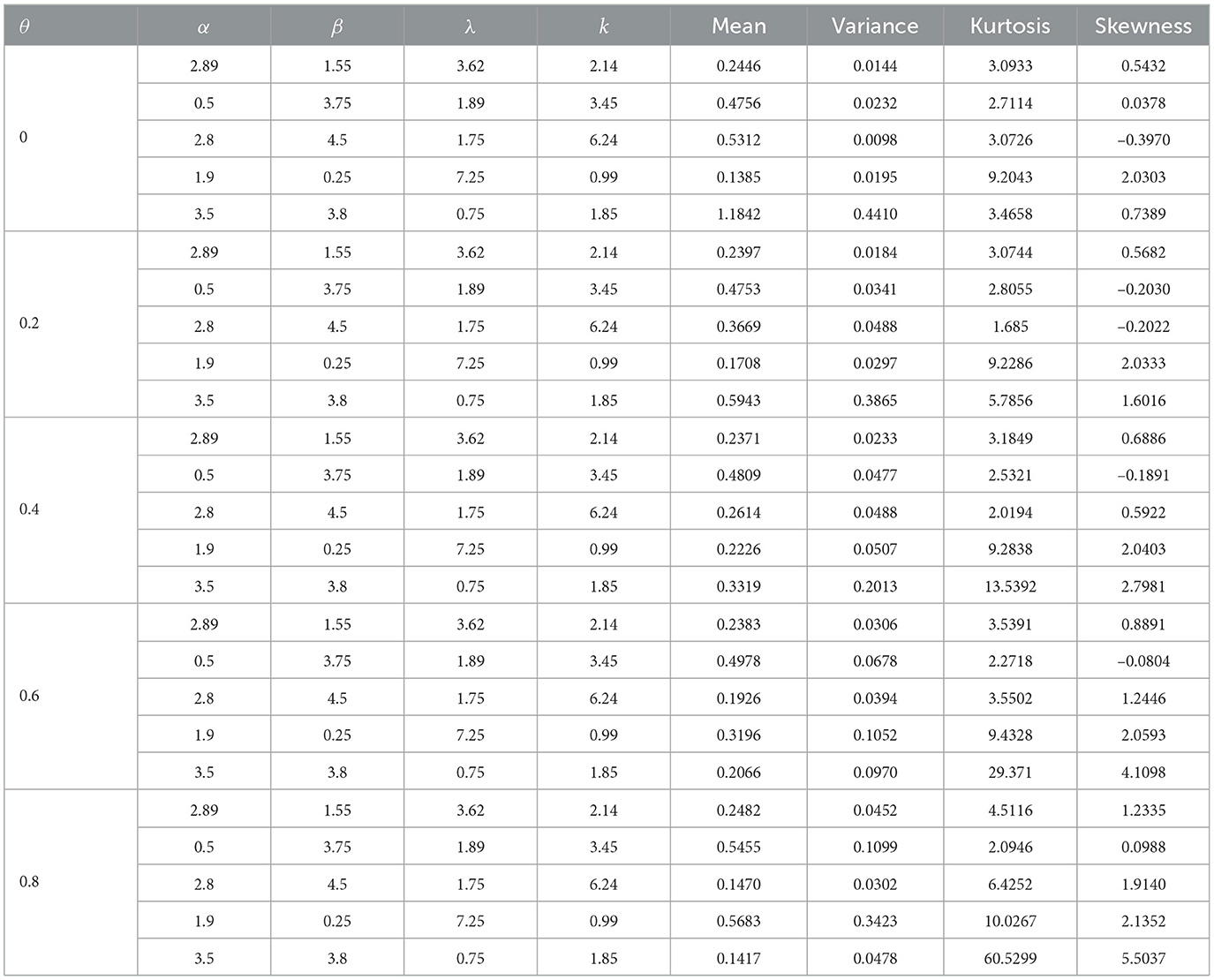
Table 3. Mean, variance, kurtosis, and skewness of θ-WMWLx distribution.
4.8 Order statistics
Suppose X(1), X(2), ⋯ , X(n) are the order statistics from the θ-WMWLx distribution. The probability density function of the i-th order statistic (with parameters suppressed) is given by
Applying the binomial expansion, we have
where [F(x)]p+i−1 can be written as
Thus, by substituting Equation (15) into Equation (14), we obtain
Subsequently, by substituting Equation (10) into Equation (16), we get
where tl, j, p and δθα(l+1), k−1(x) are, respectively, given by
and
If we set i = 1 and i = n in Equation (17), we obtain the PDF of the minimum and the PDF of the maximum of the θ-WMWLx distribution, respectively.
4.9 Estimation methods
This section presents three different methods for estimating the parameters of the proposed model: maximum likelihood estimators (MLE), least squares estimators (LSE), and weighted least squares estimators (WLSE).
4.9.1 Maximum likelihood estimators
Suppose that X1, X2, …, Xn is a random sample from θ-WMWLx distribution, the likelihood function is given by
Then, the logarithm of the likelihood function is
where ui = (1+βxi).
We obtain maximum likelihood estimates by differentiating l with respect to each parameter λ, k, α, and β and setting the result equal to zero. The partial derivatives of l with respect to each parameter or the score function are given by
These equations cannot be solved analytically. Therefore, statistical software can be used to solve them numerically.The components of the score vector Un are
The normal approximation of the maximum likelihood estimator (MLE) of Θ can be used to construct approximate confidence intervals and test hypotheses about the parameters. Under regularity conditions (see Schafer [29]), we have that
where ≈ means “approximately distributed” and is the unit information matrix. The asymptotic behavior remains valid if , where Jn(Θ) is the observed information matrix, which is replaced by the average sample information matrix evaluated at , that is, .
The elements of the main diagonal in the observed information matrix are given as follows:
Then, the asymptotic variance–covariance matrix for the maximum likelihood estimators (MLEs) is obtained by inverting the observed information matrix , or equivalently:
The approximate confidence intervals (ACI) of (1−δ)100% for the parameters are
where are the variances of , , , and , given by the diagonal elements of , and zδ/2 is the upper (δ/2) percentile of the standard normal distribution.
4.9.2 Least squares estimators
Suppose X(1), X(2), …, X(n) are ordered observations from the θ-WMWLx distribution with CDF Fθ(θ, λ, k, α, β). Then, the least squares estimators (LSE), as described by Swain et al. [30], are obtained by minimizing
with respect to the parameters λ, k, α, and β.
4.9.3 Weighted least squares estimators
Suppose X(1), X(2), …, X(n) are ordered observations from the θ-WMWLx distribution with CDF Fθ(θ, λ, k, α, β). Then, the weighted least squares estimators (WLSE), as described by Swain et al. [30], are obtained by minimizing
with respect to the parameters λ, k, α, and β.
4.10 A parsimonious special case: 1/2-WMWLx1
In this subsection, we consider a special case of the θ-WMWLx model by setting θ = 1/2 and β = 1. This particular case results in a simplified form of the PDF, defined as
The choice of θ = 1/2 and β = 1 is particularly interesting for several reasons:
Equivalent weight in the mixture: Setting θ = 1/2 grants equal weight to the reference distributions in the resulting mixture. This means that the influence of both distributions is balanced, which can simplify the analysis and provide a clearer representation of how each component contributes to the final model.
Model parsimony: Choosing β = 1 simplifies the model structure by reducing the number of parameters affecting the scale of the distribution. With β = 1, the parameter λ takes on a more central role as the sole parameter affecting the scale, favoring the parsimony of the resulting model. This parsimony can be beneficial in applications where simpler and more efficient models are preferred without the need for multiple parameters for scale or distribution shape.
Previous studies have shown inconsistencies in the maximum likelihood estimator (ML) and high estimation errors in practical applications. These issues may indicate challenges associated with model identifiability and complexity arising from multiple parameters of scale and shape. Presenting the parsimonious model 1/2-WMLx1 offers a robust and straightforward solution. This model maintains the necessary flexibility for practical applications while reducing complexity and potentially improving the stability and accuracy of estimates. Figures 5, 6 show the plots of the PDF, hazard, mean residual life, and mean inactivity time functions for the 1/2-WMWLx1 distribution with various parameter combinations. Table 4 displays the fundamental statistics of the 1/2-WMWLx1 distribution with α = 2, λ = 1, and k = 2.
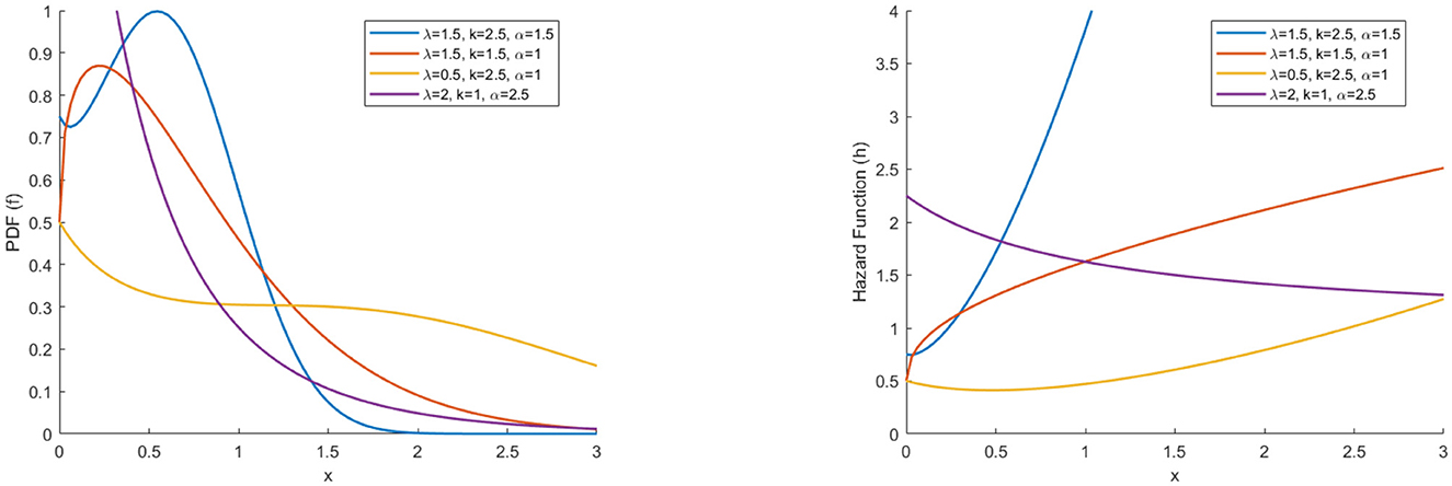
Figure 5. PDF and HRF of 1/2-WMWLx1 distribution.
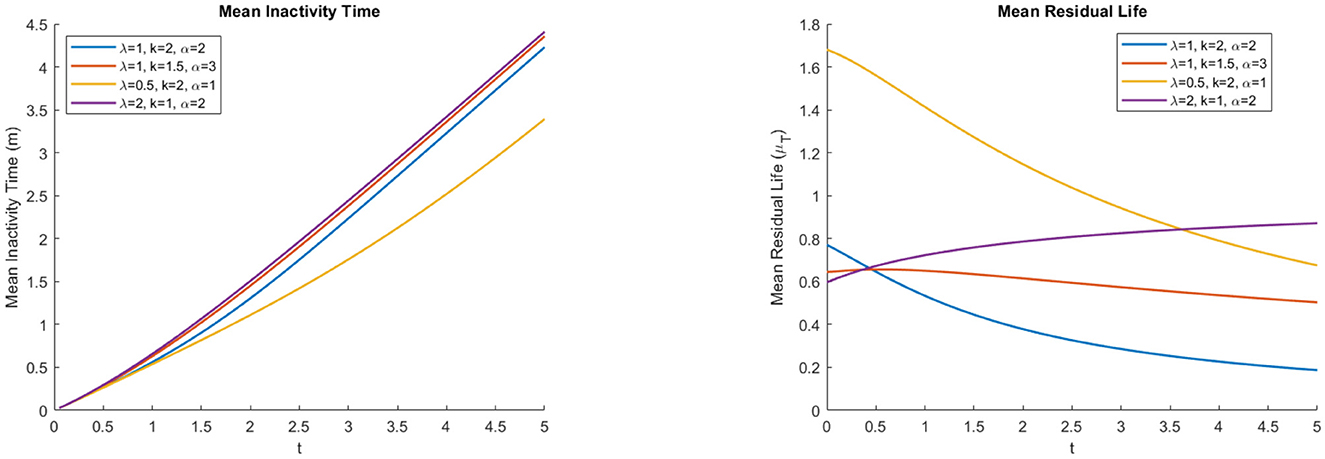
Figure 6. Mean inactivity time and residual life of the 1/2-WMWLx1 distribution.

Table 4. Basic statistics of the 1/2-WMWLx1 distribution.
5 Simulation and application
In this section, we analyze the performance of the proposed model through simulation and its application on two sets of real-world data.
5.1 Simulation
Simulations allow us to visualize the behavior of the proposed model. In this case, we conducted a simulation to analyze the performance of the maximum likelihood estimator (MLE), least squares estimators (LSE), and weighted least squares estimators (WLSE) in terms of standard errors (SE),and mean squared error (MSE) for different sample sizes and various parameter values. We generated 1,000 replications using different parameter sets with sample sizes of n = 20, n = 50, n = 100, and n = 500 from the θ-WMWLx distribution. The pseudo-random numbers are generated using the exponential distribution inverse transform method, where each number xi is sampled from an exponential distribution with rate parameter λtrue. MLE, LSE, and WLS were computed using the fminsearch function provided by MATLAB version R2024a to minimize the expressions defined in Equations (18–20) with respect to the parameters λ, k, α, and β.
The simulation results (see Tables 5, 6) indicate that the MLE method showed superior performance in terms of standard error (SE) and mean squared error (MSE) for all parameter combinations. The LSE and WLSE methods exhibited higher MSE, and their estimates were less accurate. These results highlight the robustness of MLE under various conditions.
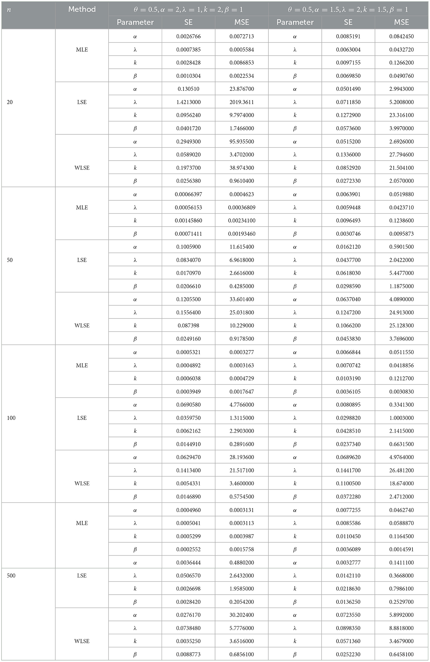
Table 5. Simulation results.
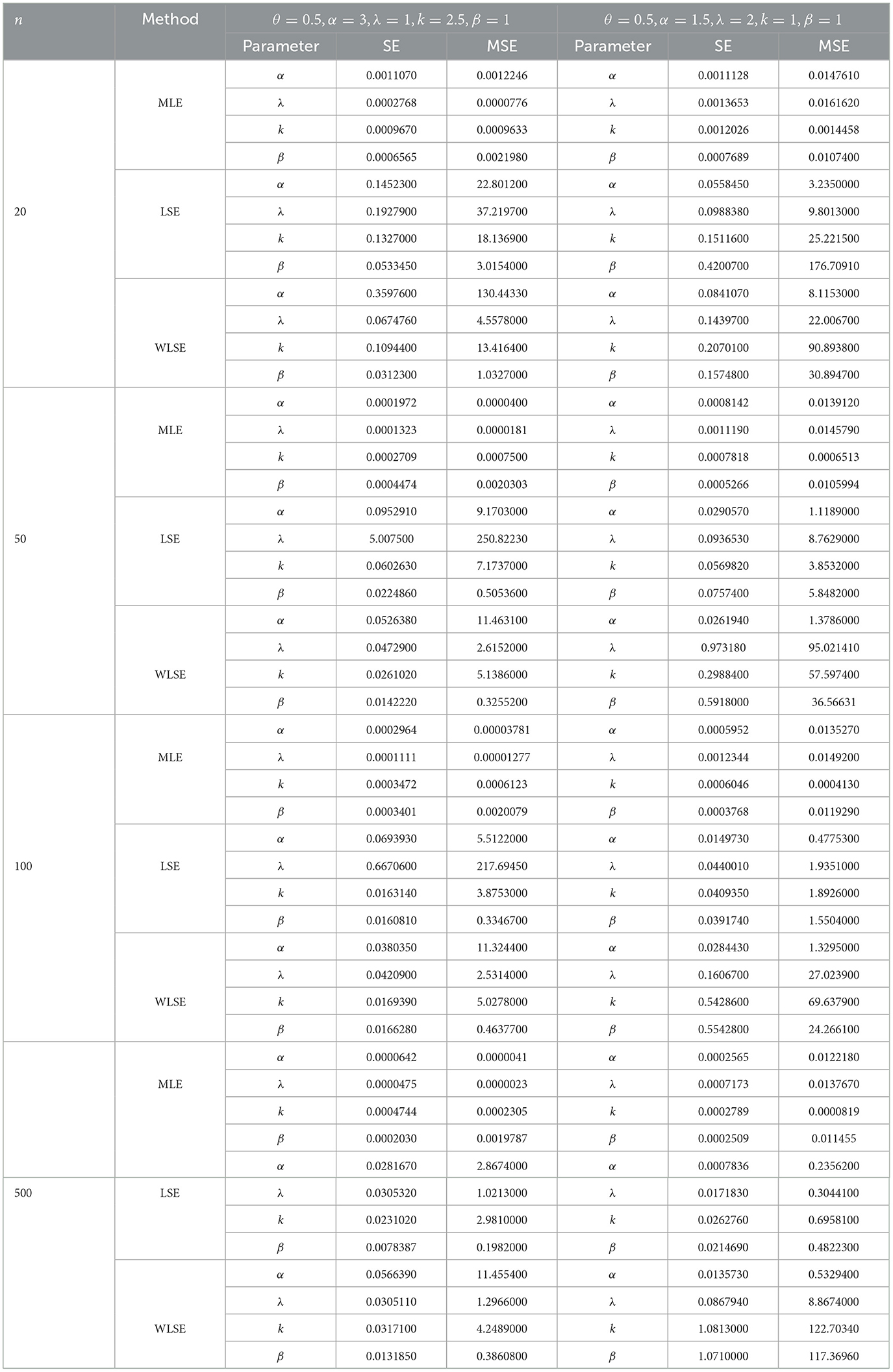
Table 6. Simulation results.
5.2 Applications on real data
In this section, we study the behavior of the θ-WMWLx distribution applied to three real datasets. We compute the maximum likelihood estimates (MLEs) for the parameters using MATLAB version R2024a's fmincon function and compare the fit with the Weibull (W), exponentiated Kumaraswamy inverse Weibull (EKIW) [31], odd Kumaraswamy inverse Weibull (OKIW) [32], Marshall-Olkin power Lomax (MOPLx) [33], Lomax-exponential distribution (LED) [34], Lomax-Rayleigh (LR) [35], Fréchet Topp-Leone Lomax (FTLLx) [36], alpha-power power-Lomax (APPLx) [37], Kumaraswamy generalized power Lomax (KPL) [38], Lomax-inverse exponential power (LIEP) [39], special case (1/2-WMWLx1), and Lomax (Lx) distributions. Below, we present the probability density functions of the mentioned distributions:
1. w:
2. EKIW: f(x|β, λ, θ, k, α) = βλθkαβx−(β+1)e(−λu)[1−e(−λu)]k−1[1−(1−e−λu)k]θ−1,where u = (α/x)β.
3. OKIW: f(x|Θ) = βkλθαβx−(β+1)[1−e1−(1−e−λu)−k]θ−1 e1−(1−e−λu)−k−λu(1−e−λu)−k−1,where Θ = (β, k, λ, θ, α), and u = (α/x)β.
4. MOPLx:
5. LED:
6. LR:
7. FTLLx: f(x|α, β, θ, k, λ) = 2αβαλθk(1+kx)−2θ−1
8. APPLx:
9. KPL:
10. LIEP:
11. Lx:
The model selection is based on the Akaike information criterion (AIC), the Bayesian information criterion (BIC), the consistent Akaike information criterion (CAIC), and the Hannan-Quinn information criterion (HQIC). In addition, as a measure of the goodness of fit, we consider the Anderson–Darling (A⋆), Cramer–von Mises (W⋆), and Kolmogorov–Smirnov (D) statistics.
5.2.1 First application: lifetime of a device
The data for this initial application consisted of 50 observations representing the lifetime of a device (see Aarset [40] for more details on the data). Here, we will compare the fits of the θ-WMWLx distribution with those of other competitive models, namely, Lx, W, LED, OKIW, EKIW, FTLLx, APPLx, KPL, and 1/2-WMWLx1. Table 7 shows the MLEs for the parameters, along with their corresponding standard errors (in parentheses), while Table 8 presents the values of the information criteria AIC, BIC, CAIC, and HQIC, as well as the goodness-of-fit statistics for the models. Figures 7, 8 illustrate the fitted densities, the boxplot, and the P–P and Q–Q plots.
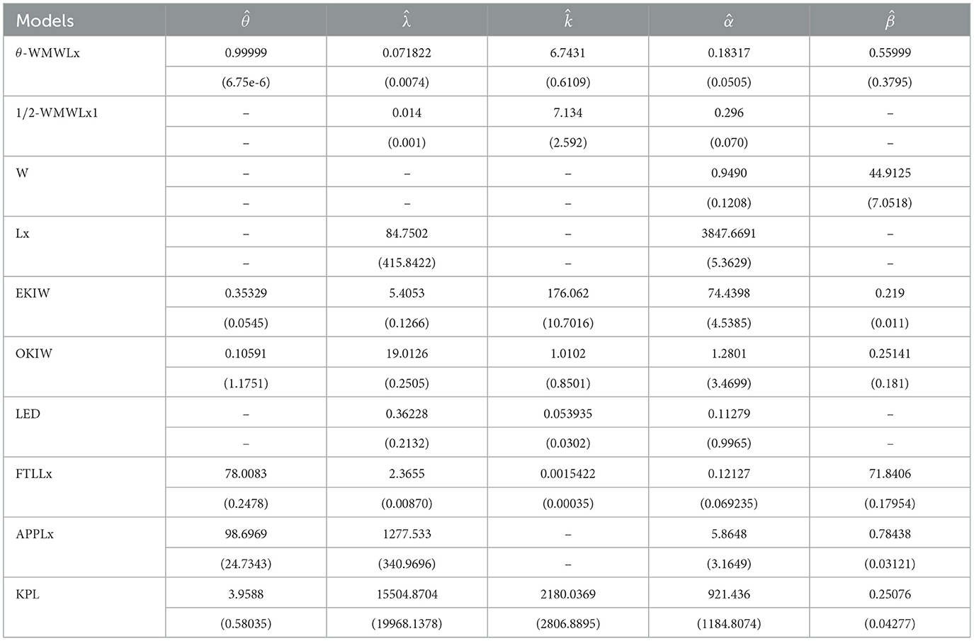
Table 7. MLEs for the first application.
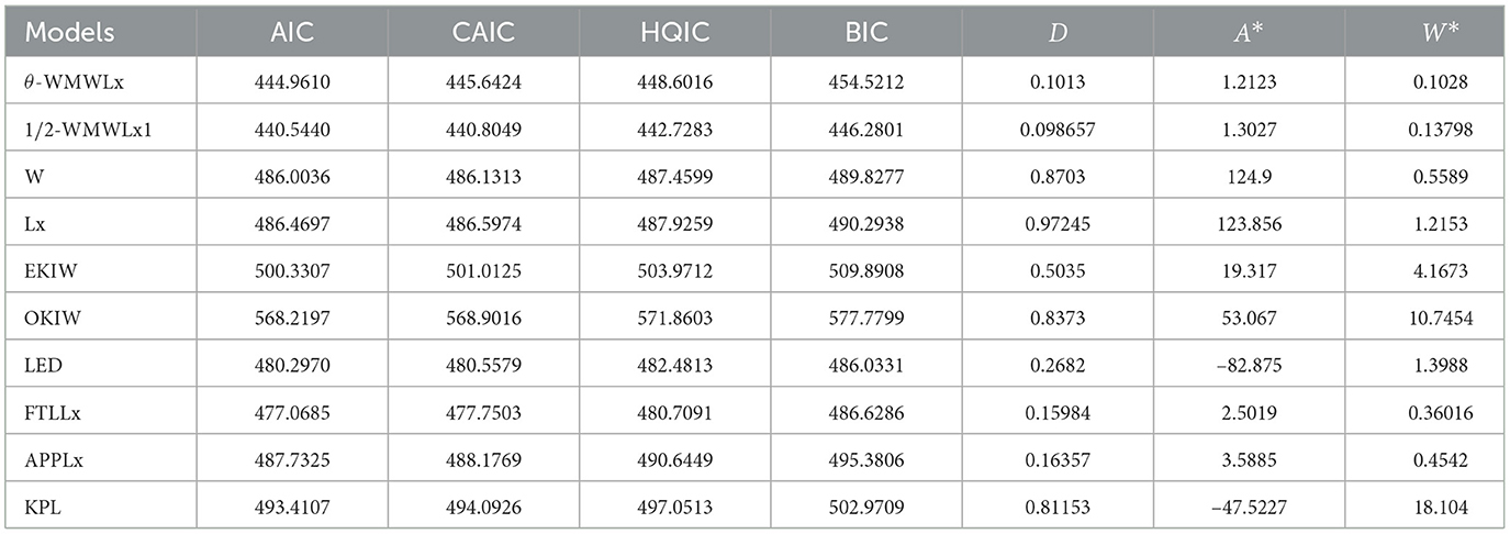
Table 8. Goodness-of-fit statistics and information criteria for the first application.
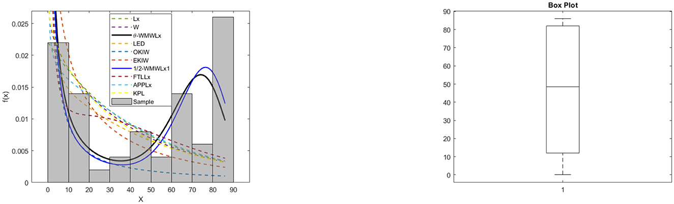
Figure 7. Fitted densities and box plot of the θ-WMWLx model for lifetime of a device.
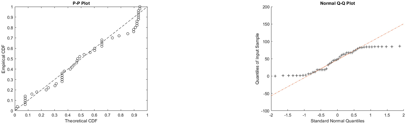
Figure 8. The P-P and Q-Q plots of the θ-WMWLx model for lifetime of a device.
5.2.2 Second application: aircraft windshield failure data
In this second application, we will use data on aircraft windshield failure times. This dataset contains 84 observations and is available in the study of Murthy et al. [41]. Tables 9, 10 show the MLEs for the parameters, along with their corresponding standard errors (in parentheses), and the goodness-of-fit statistics for the models: θ-WMWLx, W, OKIW, EKIW, MOPLx, Lx, FTLLx, KPL, LIEP, and 1/2-WMWLx1. In addition, Figures 9, 10 illustrate the fitted densities, the boxplot, and the P–P and Q–Q plots.
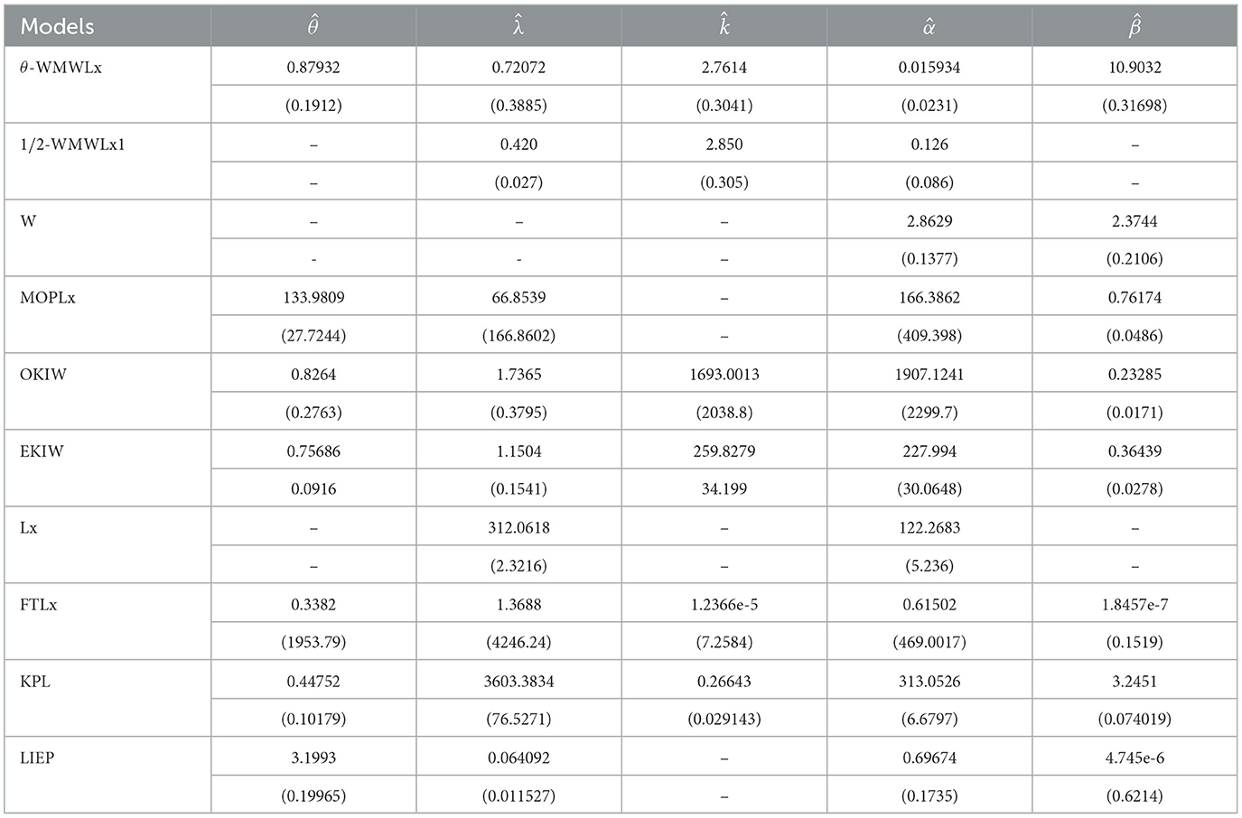
Table 9. MLEs for the second application.
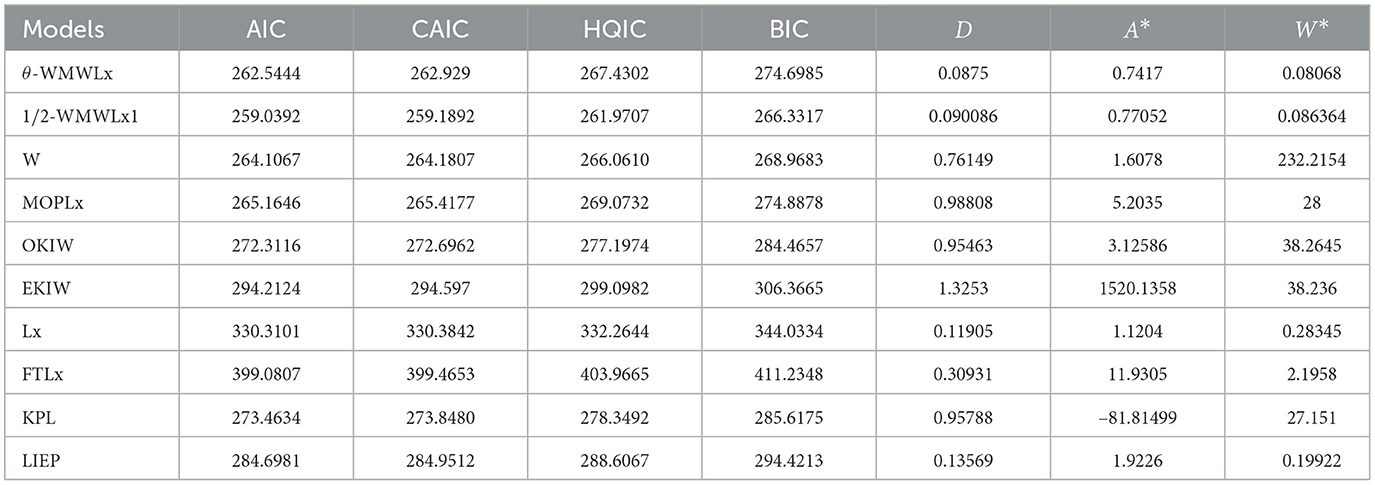
Table 10. Goodness-of-fit statistics and information criteria for the second application.
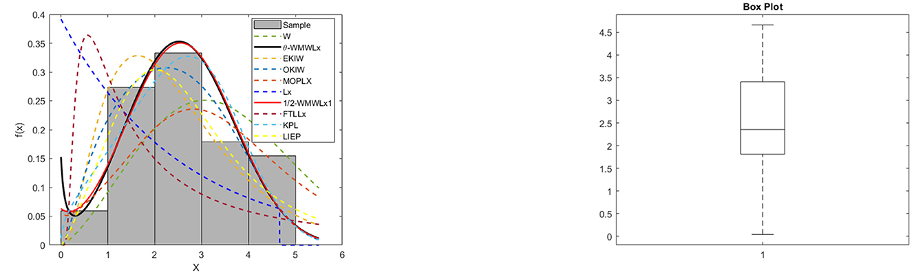
Figure 9. Fitted densities and box plot of the θ-WMWLx model for aircraft windshield failure time.
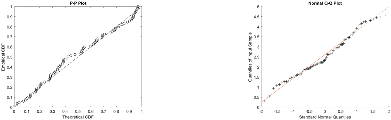
Figure 10. P-P and Q-Q plots of the θ-WMWLx model for aircraft windshield failure time.
5.2.3 Third application: milk production
In this application, we utilized a dataset concerning the total milk production in the first birth of 107 cows from SINDI race. Please refer to Yousof et al. [42]. Tables 11, 12 show the MLEs for the parameters, accompanied by their respective standard errors (in parentheses), and the goodness-of-fit statistics for the following models: θ-WMWLx, W, OKIW, EKIW, MOPLx, LR, Lx, FTLLx, APPLx, KPL, LIEP, and 1/2-WMWLx1. In addition, Figure 11 and Table 12 illustrate the fitted densities, the box plot, as well as the P-P and Q-Q plots.
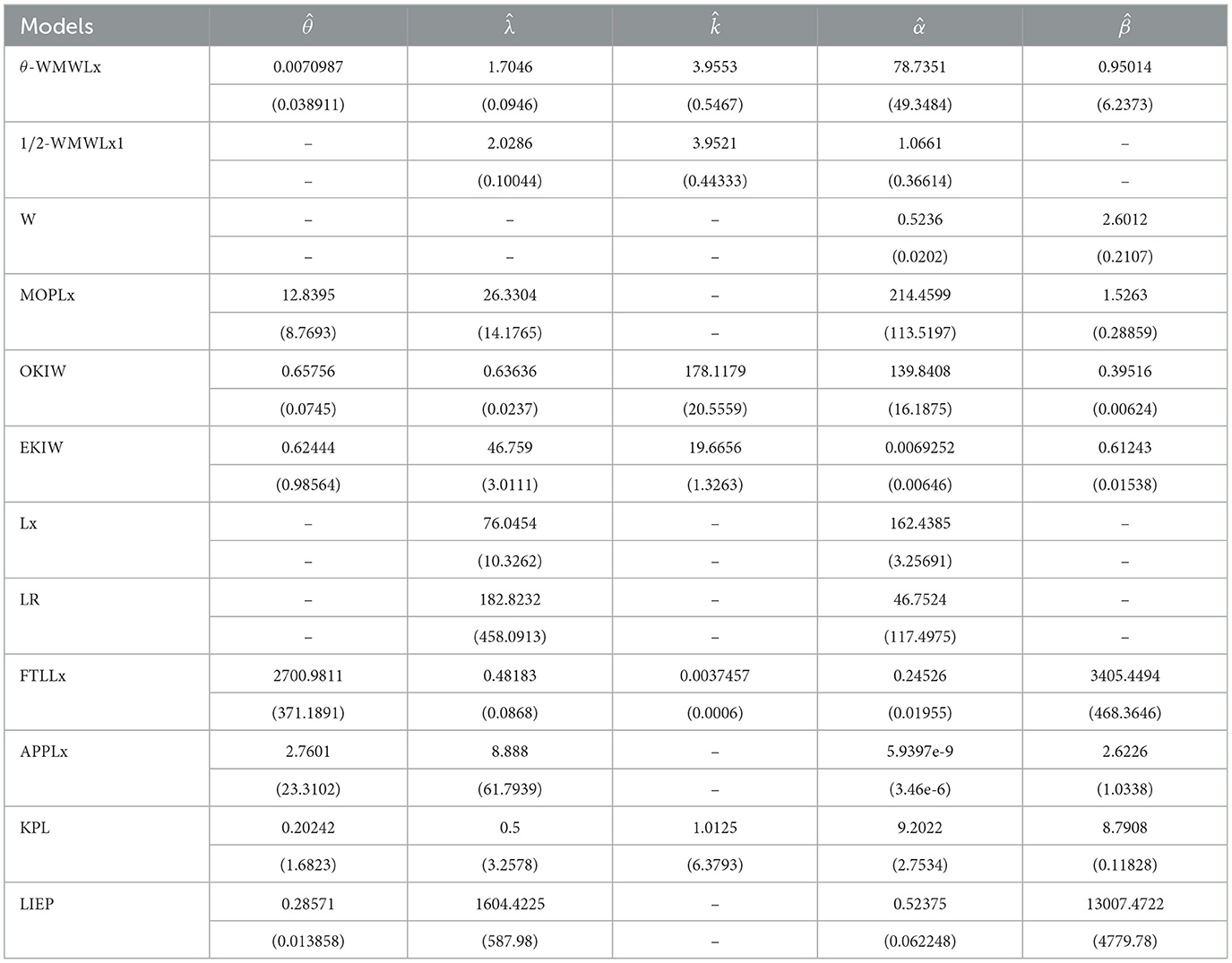
Table 11. MLEs for the third application.

Table 12. Goodness-of-fit statistics and information criteria for the third application.
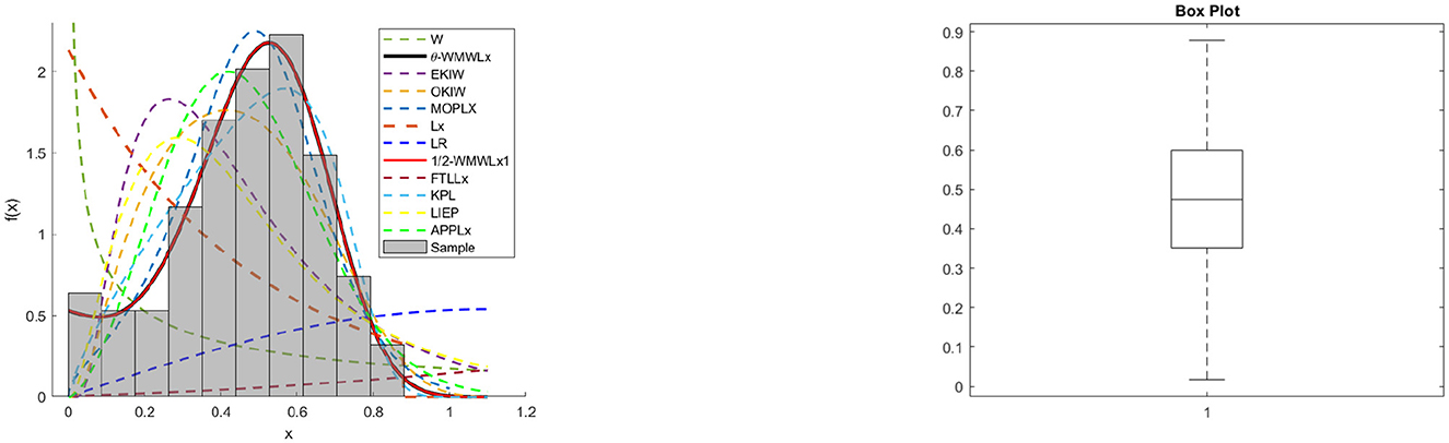
Figure 11. Fitted densities and box plot of the θ-WMWLx model for milk production.
The results presented in Tables 8, 10, 12 indicate that the θ-WMWLx distribution consistently shows the lowest values in information criteria (AIC, BIC, CAIC, and HQIC) compared to its competitor counterparts. This pattern is equally reflected in the goodness-of-fit statistics, where the θ-WMWLx distribution excels. Therefore, we can conclude that the θ-WMWLx distribution offers the most optimal fit for these three datasets.
On the other hand, the graphs in Figures 7–12 reveal that the θ-WMWLx distribution fits more accurately to the three datasets studied compared to other competing models. This observation further reinforces the superiority of the θ-WMWLx distribution in terms of fitting capability and predictive accuracy.
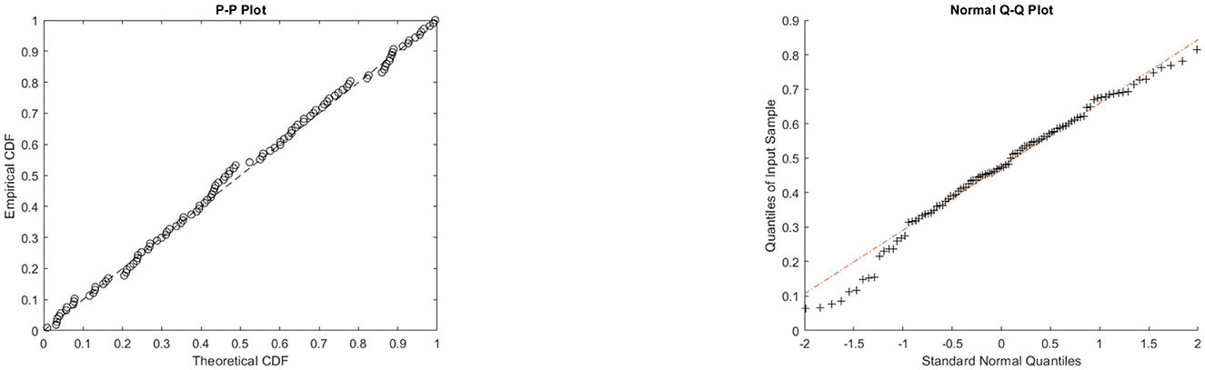
Figure 12. P-P and Q-Q plots of the θ-WMWLx model for milk production.
6 Conclusion and comments
The research introduces the family of θ-weighted mixture distributions, offering a flexible approach to modeling the joint distribution of random variables. This family combines survival functions from baseline distributions, resulting in diverse shapes and characteristics determined by the parameters' behavior. A specific case, θ-WMWLx, was investigated, combining the survival functions of the Weibull and Lomax distributions, revealing a spectrum of shapes, from symmetric to asymmetric, with various biases.
Statistical properties and reliability aspects of θ-WMWLx were examined, demonstrating that an increase in sample size enhances the precision of the maximum likelihood estimator (MLE). The significance of the parameter θ in shaping and fitting the resulting distribution is underscored, posing a future challenge to explore methods for determining its optimal value, which could enhance the utility of this methodology.
A notable special case is the 1/2-WMWLx1, which simplifies the model structure by balancing the weight of the baseline distributions and reducing the number of parameters affecting the scale. This parsimony can be beneficial in practical applications by improving the stability and accuracy of the estimates, facilitating a clearer and more efficient analysis. This was reflected in the application section of the study, where this special case, along with the general case, proved to be the best in terms of performance.
In addition to the aforementioned aspects, several additional research challenges could be addressed in future studies. One such challenge could involve generalizing the proposed model to accommodate a broader range of baseline distributions, allowing for greater flexibility in modeling various data types. Furthermore, a more in-depth analysis of the survival and hazard functions using the θ-WMWLx could be conducted, exploring how these functions vary across different parameter settings and how they can contribute to a better understanding of data behavior in diverse scenarios. These endeavors could advance our comprehension of the joint distribution of random variables and foster the development of more effective tools for their modeling and analysis across various applied contexts.
Data availability statement
The original contributions presented in the study are included in the article/supplementary material, further inquiries can be directed to the corresponding author.
Author contributions
CC-M: Writing – original draft, Writing – review & editing. RM: Writing – original draft, Writing – review & editing. EC: Writing – original draft, Writing – review & editing.
Funding
The author(s) declare financial support was received for the research, authorship, and/or publication of this article. This work was supported by Universidad de Playa Ancha, Plan de Fortalecimiento Universidades Estatales - Ministerio de Educación, convenio UPA 1999.
Acknowledgments
The authors would like to thank the Support Network of the General Directorate of Research for their cooperation in reviewing this article.
Conflict of interest
The authors declare that the research was conducted in the absence of any commercial or financial relationships that could be construed as a potential conflict of interest.
Publisher's note
All claims expressed in this article are solely those of the authors and do not necessarily represent those of their affiliated organizations, or those of the publisher, the editors and the reviewers. Any product that may be evaluated in this article, or claim that may be made by its manufacturer, is not guaranteed or endorsed by the publisher.
References
1. Pearson K. Contributions to the mathematical theory of evolution. Philos Trans R Soc Lond A. (1894) 185:71–110. doi: 10.1098/rsta.1894.0003
2. Amoroso L. Ricerche intorno alla curva dei redditi. Ann Mat Pura Appl. (1925) 2:123–59. doi: 10.1007/BF02409935
3. Burr IW. Cumulative frequency functions. Ann Math Stat. (1942) 13:215–32. doi: 10.1214/aoms/1177731607
4. Johnson NL. Systems of frequency curves generated by methods of translation. Biometrika. (1949) 36:149–76. doi: 10.1093/biomet/36.1-2.149
5. Marshall AW, Olkin I. A new method for adding a parameter to a family of distributions with application to the exponential and Weibull families. Biometrika. (1997) 84:641–52. doi: 10.1093/biomet/84.3.641
6. Okasha HM, Kayid M. A new family of Marshall-Olkin extended generalized linear exponential distribution. J Comput Appl Math. (2016) 296:576–92. doi: 10.1016/j.cam.2015.10.017
7. Jose KK, Krishna E. Marshall-Olkin extended uniform distribution. In: ProbStat Forum, Vol. 4. (2011), p. 78–88.
8. Sengweni W, Oluyede B, Makubate B. The Marshall-Olkin Topp-Leone Half-Logistic-G family of distributions with applications. Stat Optim Inf Comput. (2023) 11:1001–26. doi: 10.19139/soic-2310-5070-1082
9. Handiquea L, Chakraborty S, El-Morshedy M, Afifyd AZ, Eliwa MS. Modelling veterinary medical data utilizing a new generalized Marshall-Olkin transmuted generator of distributions with statistical properties. Thail Stat. (2024) 22:219–36.
10. Shaw WT, Buckley IR. The alchemy of probability distributions: beyond Gram-Charlier expansions, and a skew-kurtotic-normal distribution from a rank transmutation map. arXiv. (2009). [Preprint]. arXiv:09010434. doi: 10.48550/arXiv:09010434
11. Afify AZ, Al-Mofleh H, Aljohani HM, Cordeiro GM. The Marshall-Olkin-Weibull-H family: estimation, simulations, and applications to COVID-19 data. J King Saud Univ-Sci. (2022) 34:102115. doi: 10.1016/j.jksus.2022.102115
12. Barreto-Souza W, Lemonte AJ, Cordeiro GM. General results for the Marshall and Olkin's family of distributions. An Acad Bras Ciênc. (2013) 85:3–21. doi: 10.1590/S0001-37652013000100002
13. Souza L, Junior W, De Brito C, Chesneau C, Ferreira T, Soares L. On the Sin-G class of distributions: theory, model and application. J Math Model. (2019) 7:357–79. doi: 10.22124/jmm.2019.13502.1278
14. Shama MS, El Ktaibi F, Al Abbasi JN, Chesneau C, Afify AZ. Complete study of an original power-exponential transformation approach for generalizing probability distributions. Axioms. (2023) 12:67. doi: 10.3390/axioms12010067
15. Nadarajah S, Kotz S. The exponentiated type distributions. Acta Applicandae Mathematica. (2006) 92:97–111. doi: 10.1007/s10440-006-9055-0
16. Eugene N, Lee C, Famoye F. Beta-normal distribution and its applications. Commun Stat-Theory Methods. (2002) 31:497–512. doi: 10.1081/STA-120003130
17. Cordeiro GM, de Castro M. A new family of generalized distributions. J Stat Comput Simul. (2011) 81:883–98. doi: 10.1080/00949650903530745
18. Mahdavi A, Kundu D. A new method for generating distributions with an application to exponential distribution. Commun Stat-Theory Methods. (2017) 46:6543–57. doi: 10.1080/03610926.2015.1130839
19. Iriarte YA, de Castro M, Gómez HW. The Lambert-F distributions class: An alternative family for positive data analysis. Mathematics. (2020) 8:1398. doi: 10.3390/math8091398
20. Tahir MH, Cordeiro GM, Mansoor M, Zubair M. The Weibull-Lomax distribution: properties and applications. Hacet J Math Stat. (2015) 44:455–74. doi: 10.15672/HJMS.2014147465
21. Afify AZ, Nofal ZM, Yousof HM, El Gebaly YM, Butt NS. The transmuted Weibull Lomax distribution: properties and application. Pak J Stat Oper Res. (2015) XI:135–52. doi: 10.18187/pjsor.v11i1.956
22. Hassan AS, Abd-Allah M. Exponentiated Weibull-Lomax distribution: properties and estimation. J Data Sci. (2018) 16:277–98. doi: 10.6339/JDS.201804_16(2).0004
23. Ijaz M, Asim SM, Alamgir. Lomax exponential distribution with an application to real-life data. PLoS ONE. (2019) 14:e0225827. doi: 10.1371/journal.pone.0225827
24. Alzaghal A, Ghosh I, Alzaatreh A. On shifted Weibull-Pareto distribution. Int J Stat Probab. (2016) 5:139–49. doi: 10.5539/ijsp.v5n4p139
25. Kartsonaki C. Survival analysis. Diagn Histopathol. (2016) 22:263–70. doi: 10.1016/j.mpdhp.2016.06.005
26. Baredar P, Khare V, Nema S. Design and Optimization of Biogas Energy Systems. Cambridge, MA: Academic Press (2020). doi: 10.1016/B978-0-12-822718-3.00001-0
27. Kayid M, Al-Nahawati H, Ahmad IA. Testing behavior of the reversed hazard rate. Appl Math Model. (2011) 35:2508–15. doi: 10.1016/j.apm.2010.11.054
28. Alshangiti AM, Kayid M, Alarfaj B. A new family of Marshall-Olkin extended distributions. J Comput Appl Math. (2014) 271:369–79. doi: 10.1016/j.cam.2014.04.020
29. Schafer RE. Statistical Models and Methods for Lifetime Data. New York, NY: Taylor & Francis (1983). doi: 10.2307/1267739
30. Swain JJ, Venkatraman S, Wilson JR. Least-squares estimation of distribution functions in Johnson's translation system. J Stat Comput Simul. (1988) 29:271–97. doi: 10.1080/00949658808811068
31. Rodrigues J, Silva APCM, Hamedani G. The exponentiated Kumaraswamy inverse Weibull distribution with application in survival analysis. J Stat Theory Appl. (2016) 15:8–24. doi: 10.2991/jsta.2016.15.1.2
32. Atem BAM. On the odd Kumaraswamy inverse Weibull distribution with application to survival data. JKUAT. (2018). doi: 10.17654/AS051050309
33. Ul Haq MA, Hamedani G, Elgarhy M, Ramos PL. Marshall-Olkin Power Lomax distribution: Properties and estimation based on complete and censored samples. Int J Stat Probab. (2020). doi: 10.5539/ijsp.v9n1p48
34. Hami Golzar N, Ganji M, Bevrani H. The Lomax-exponential distribution, some properties and applications. J Stat Res Iran JSRI. (2017) 13:131–53. doi: 10.18869/acadpub.jsri.13.2.131
35. Venegas O, Iriarte YA, Astorga JM, Gómez HW. Lomax-Rayleigh distribution with an application. Appl Math Inf Sci. (2019) 13:741–8. doi: 10.18576/amis/130506
36. Reyad H, Korkmaz MÇ, Afify AZ, Hamedani G, Othman S. The Fréchet Topp Leone-G family of distributions: Properties, characterizations and applications. Ann Data Sci. (2021) 8:345–66. doi: 10.1007/s40745-019-00212-9
37. Qura ME, Alqawba M, Al Sobhi MM, Afify AZ. A novel extended power-Lomax distribution for modeling real-life data: properties and inference. J Math. (2023) 2023:6661792. doi: 10.1155/2023/6661792
38. Nagarjuna VB, Vardhan RV, Chesneau C. Kumaraswamy generalized power Lomax distributionand its applications. Stats. (2021) 4:28–45. doi: 10.3390/stats4010003
39. Sapkota LP, Kumar V, Gemeay AM, Bakr M, Balogun OS, Muse AH. New Lomax-G family of distributions: statistical properties and applications. AIP Adv. (2023) 13:095128. doi: 10.1063/5.0171949
40. Aarset MV. How to identify a bathtub hazard rate. IEEE Trans Reliab. (1987) 36:106–8. doi: 10.1109/TR.1987.5222310
Keywords: mixture distribution, Weibull distribution, Lomax distribution, survival function, distribution family
Citation: Carvajal-Muquillaza C, Manríquez R and Cabrera E (2024) θ-Weighted mixture distribution: the Weibull-Lomax case. Front. Appl. Math. Stat. 10:1418589. doi: 10.3389/fams.2024.1418589
Received: 16 April 2024; Accepted: 16 July 2024;
Published: 07 August 2024.
Edited by:
Artur Lemonte, Federal University of Rio Grande do Norte, BrazilReviewed by:
Ahmed Z. Afify, Benha University, EgyptYuri A. Iriarte, Universidad de Antofagasta, Chile
Copyright © 2024 Carvajal-Muquillaza, Manríquez and Cabrera. This is an open-access article distributed under the terms of the Creative Commons Attribution License (CC BY). The use, distribution or reproduction in other forums is permitted, provided the original author(s) and the copyright owner(s) are credited and that the original publication in this journal is cited, in accordance with accepted academic practice. No use, distribution or reproduction is permitted which does not comply with these terms.
*Correspondence: Cristian Carvajal-Muquillaza, Y3Jpc3RpYW4uY2FydmFqYWxAdXBsYS5jbA==