The generalized STAR modeling with minimum spanning tree approach of spatial weight matrix

The weight matrix is one of the most important things in Generalized Space–Time Autoregressive (GSTAR) modeling. Commonly, the weight matrix is built based on the assumption or subjectivity of the researchers. This study proposes a new approach to composing the weight matrix using the minimum spanning tree (MST) approach. This approach reduces the level of subjectivity in constructing the weight matrix since it is based on the observations. The spatial dependency among locations is evaluated through the centrality measures of MST. It is obtained that this approach could give a similar weight matrix to the commonly used, even better in some ways, especially in modeling the data with higher variability. For the study case in traffic problems, the number of vehicles entering the Purbaleunyi toll was modeled by GSTAR with several weight matrix perspectives. According to Space–Time ACF-PACF plots, GSTAR(1;1), GSTAR(1,2), and GSTAR(2;1,1) models are the candidates for appropriate models. Based on the root mean square errors and mean absolute percentage errors, it is concluded that the GSTAR(2,1,1) with MST approach is the best model to forecast the number of vehicles entering the Purbaleunyi toll. This best model is followed by GSTAR(1,1) with an MST approach of spatial weight matrix.

1 Introduction

The Generalized Space–Time Autoregressive (GSTAR) is one of the methods to analyze the space–time series. This model adapted the vector autoregressive model, which, instead of involving many variables, considered time series in many locations simultaneously. The development of the GSTAR model in Indonesia is very fast, both in theory and application. The theory includes process stationarity properties using inverse autocovariance matrix in (1) and the kernel approach in (2); the GSTAR with heteroscedastic effect in (3, 4); and the weight matrix construction of the GSTAR model using the kernel approach in (5) and graph in (6). The development of the GSTAR model with correlated errors is in (7, 8). The GSTAR model with exogenous variables and outliers is in (9), the Poisson GSTAR in (10), the optimal spatial aggregation of GSTARMA model in (11), the higher order model in (12), and the GSTAR for discrete data in (13). The application of the GSTAR model has been carried out on economic data in (14), tea plantation production in (15), oil palm production in (16), commodity prices of red chilies in (17), rainfall data of West Java in (18), number of dengue fever cases in (19), “Begal” criminal cases in Medan, North Sumatera, in (20), variation of Northern Ethiopia’s temperature in (21), and the number of COVID-19 cases in Java island in (6, 22).

This model’s basic assumption is the existence of spatial dependence among observed locations. In addition to the spatial autoregressive parameters, the dependence among locations is described by the spatial weight matrix. Most of the time, this matrix is simply composed based on the researcher’s subjectivity. This matrix can be classified as uniform, binary, and non-uniform weight matrix (23). The development of a weight matrix using the kernel approach is to less subjectivity (5). The weight matrix is composed based on the observations. Thus, the obtained weight matrix can be considered more objective than the conventional weight matrix. This study proposes another way to construct the weight matrix using the observations. This method constructs the minimum spanning tree (MST) graph to obtain the spatial dependence among locations through its adjacency matrix.

To obtain the description of this new approach application, the number of vehicles entering the Purbaleunyi toll gates of Bandung—West Java data is used. As the capital city of West Java, Indonesia, Bandung is one of the busiest cities on Java Island. Bandung is well-known as the center of art and music, education, business, culinary, and tourism. However, its citizens experience traffic jams every day, and the peak congestion occurs on the weekends because many people come from outside Bandung. Due to its geographic location, land transportation is more favorable to access this city. Thus, the Purbaleunyi toll gates are crowded by numerous vehicles passing every day. The space–time analysis is applied to capture this phenomenon since the occurrences are related to time and locations. There are eight toll gates involved, and the locations of those eight gates can be seen in Figure 1. It can be seen that all toll gates are connected to each other with various distances and eccentricities. Thus, the traffic route modeling of those toll gates satisfies the basic graph properties necessary to make use of MST. Some research studies regarding traffic flow forecasting with different methods are the neural network bagging ensemble hybrid modeling (24), threshold autoregression (TAR) (25), stacked autoencoder (SAE) of deep learning model (26), GSTAR model with time-correlated errors (27), segment-based data imputation (28), queueing networks (29), long short-term memory network (LSTM) (30), and multi-view travel time prediction (MVPPT) (31).

Figure 1

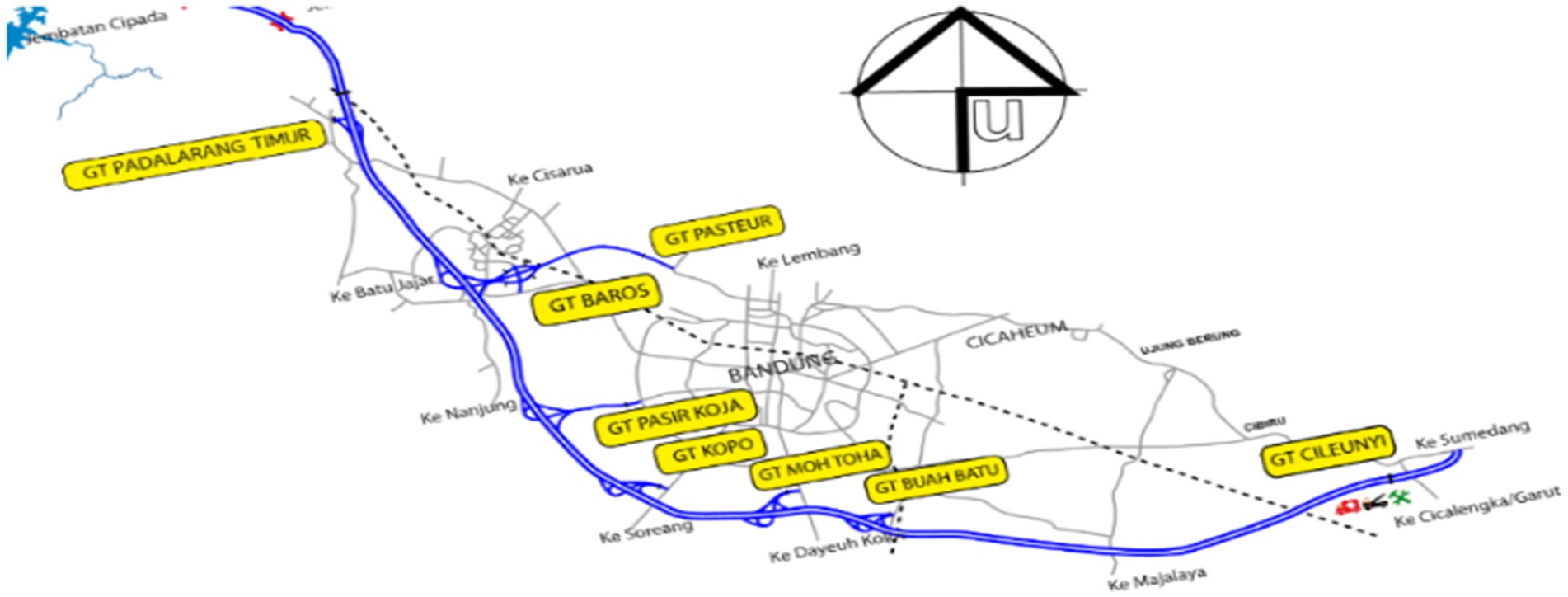
Figure 1. Map of eight gates in Purbaleunyi Toll (source: www.jasamarga.com/public/id/infolayanan/TOLl/ruas.aspx, Accessed 29 April 2018).

This study aims to determine the best space–time model that can be used to predict the number of vehicles entering the Purbaleunyi toll. There are eight toll gates involved: Padalarang (PDL), Pasteur (PST), Baros (BAR), Pasir Koja (PKJ), Kopo (KPO), M. Toha (MTH), Buah Batu (BBT), and Cileunyi (CLY). First, the new procedure is applied to obtain the spatial weight matrix using the adjacency matrix and MST graph approach. The novelty of this research is that both theory and application are new in statistical space–time modeling. This procedure is explained in Section 2. Then, in Section 3, the model selection improvement is investigated by checking the stationarity of all possible models using the inverse of autocovariance matrix (IAcM). Finally, the case study is discussed in Section 4.

2 Materials and methods

2.1 The spatial weight matrix

2.1.1 The spatial lag and conventional weight matrix

The spatial lag is constructed for all observation locations and can be obtained in many ways. A well-known method is applying the radius system, as illustrated in Figure 2. The locations closer to the reference location (s₀ ${\mathrm{s}}_0$ ) will have a smaller spatial lag, distinguished by a fixed distance, d₀ ${\mathrm{d}}_0$ . The distinct configuration of each spatial lag order may give different weight matrices.

Figure 2

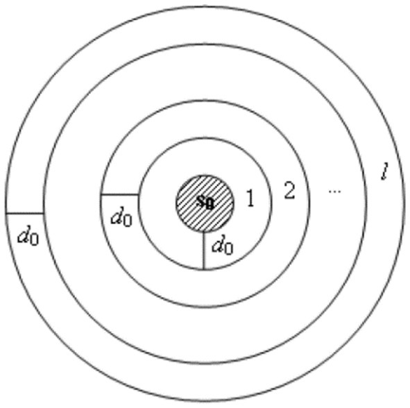
Figure 2. The radius system in determining the spatial lag. The neighbors of a reference location are classified in the same spatial lag if they lie in the same radius (23).

The weight matrix is a square matrix of size $N$ , with the following properties: (i) the diagonal entries of weight matrix $W$ are zeros, (ii) the sum of weight values in one row must equal to zero or ${\displaystyle \sum }_{j=1}^N{w}_{ij}$ = 1. For all locations $S_i$ , $i=1,2,\dots N$ , and (iii) every weight value is non-negative, or $w_{ij}\ge 0$ .

In general, there are three weight matrix types: binary, uniform, and non-uniform. The binary weight matrix consists of 0 and 1 values in off-diagonal entries, of which 1 represents the most influential neighbor. The element in the uniform weight matrix is defined as follows:

${w_{ij\text{ (1)}}}^{\left(\mathcal{𝓁}\right)}=\{\begin{array}{c}\hfill \frac{1}{{n_i}^{\left(\mathcal{𝓁}\right)}},j\mathrm{is}\mathrm{neighbor}\mathrm{of}i\mathrm{in}\mathcal{𝓁}\mathrm{t}\mathrm{h}\mathrm{order}\hfill \\ \hfill 0,\mathrm{otherwise}\hfill \end{array}$

where $n_i^{\left(\mathcal{𝓁}\right)}$ represents the number of neighbors for location i in $\mathcal{𝓁}$th spatial lag.

There are some ways to determine the non-uniform weight matrix. The simplest way is by involving the distance between locations, such as inverse distance weight, that is

${w_{ij\text{ (2)}}}^{\left(\mathcal{𝓁}\right)}=\{\begin{array}{cc}\hfill \frac{\frac{1}{1+d_{ij}^{\left(\mathcal{𝓁}\right)}}}{{{\displaystyle \sum }}_{j=1}^N\frac{1}{1+d_{ij}^{\left(\mathcal{𝓁}\right)}}},\hfill & \hfill j\mathrm{is}\mathrm{the}\mathrm{neighbor}\mathrm{of}i\mathrm{in}\mathcal{𝓁}\mathrm{t}\mathrm{h}\mathrm{order}\hfill \\ \hfill 0,\hfill & \hfill \mathrm{otherwise}\hfill \end{array}$

for location i and j in $\mathcal{𝓁}$th spatial lag which Euclidean distance is $d_{ij}^{\left(\mathcal{𝓁}\right)}$ . Since the distance is fixed, then the obtained weight matrix is also fixed. This construction could not accommodate some changes that happened in the observations. The new approach is constructed to accommodate the pattern of the observations by using an MST graph. Some previous research studies regarding the MST approach for spatial weight matrix have been investigated by (6, 32).

2.1.2 Minimum spanning tree

A graph (G) is not an empty set that makes a node at the endpoint vertices. The G is a simple graph if there are no circles and two lines that merge into a pair of vertices. If an edge can combine every vertice in a simple graph, it is called a completed graph. A tree (T) is a connecting graph without any repetition/cycle. Thus, every two vertices will be connected by one unique path. The minimum spanning tree (MST) is a connected and undirected graph. MST is a collection of lines and dots with a line consisting of an undirected weight that connects all vertices and does not contain a cycle that produces the smallest value (33). Some methods to construct the MST include the Prim and Kruskal algorithms. The common idea of both algorithms is selecting the graph with the smallest weight and connected vertices that do not form a circle. Kruskal’s algorithm is formed by adding the smallest weight of lines into the tree one by one, while the Prim algorithm is built by minimizing the weight of the connected lines. Both algorithms are simple and popular methods for constructing MST. However, they produce only an MST from all possible MSTs; thus, the uniqueness of MST could not be obtained. Therefore, an algorithm was proposed to construct a forest graph consisting of all possible MSTs using fuzzy relations (34). This algorithm is called sub-dominant ultrametric (SDU).

One of the important steps in MST construction is defining the weight of lines. Here, the weight is determined by using a distance matrix. This distance matrix can be extracted from the correlation matrix. For example, supposedly two random variables are X and Y, then, the correlation between both variables is defined as follows:

${\rho }_{X,Y}=\mathit{corr}\left(X,Y\right)=\frac{E\left[XY\right]-E\left[X\right]E\left[Y\right]}{\sqrt{E\left[X^2\right]-{\left(E\left[X\right]\right)}^2}\sqrt{E\left[Y^2\right]-{\left(E\left[Y\right]\right)}^2}}$

The correlation represents the linear dependence between variables, with values in $0\le \left|{\rho }_{X,Y}\right|\le 1$ . If both variables have strong linear dependence, the correlation values tend to be one and otherwise zero. In space–time data, the random variables are represented by the time series of each location. Consider N locations with time series realizations $\left\{z_i\left(t\right)\right\},i=1,2,\dots ,N\}$ , then the correlation between series in locations i and j is defined as follows:

$c\left(i,j\right)=\frac{z_i{z}_j-z_i{z}_j}{\sqrt{z_i^2-{z_i}^2}\sqrt{z_j^2-{z_j}^2}}$

with $z_i$ is the average of $z_i\left(t\right)$ . The $c\left(i,j\right)$ can be a sample correlation between series in locations i and j. The distance matrix $\mathrm{D}=\left\{d\left(i,j\right)\right\}$ is symmetric whose entries are defined as follows:

$d\left(i,j\right)=\sqrt{2\left(1-c\left(i,j\right)\right)}$

for all $i,j=1,2,\dots ,N$ . This distance matrix is symmetric and anti-reflexive fuzzy.

2.1.3 Spatial lag classification using MST

The spatial lag membership for a reference location using MST is based on the number of lines connected from the reference location to its neighbors. If a location is directly connected to a reference location, that location is in the first spatial lag. Thus, if ℓ lines connect the neighbor to the reference location, then this neighbor is classified as the member of spatial lag $\mathcal{𝓁}$th of the reference location.

Figure 3 shows the procedure of this spatial lag classification using MST. If the Pasir Koja toll gate is considered as the reference location, then the Pasteur toll gate is a member of its first spatial lag, and Padalarang, Kopo, M. Toha, and Baros are the members of the second spatial lag. Finally, the Cileunyi toll gate will be in the third spatial lag, and Buah Batu is the only member of the fourth spatial lag. After determining the number of memberships in the spatial lag $\mathcal{𝓁}$th for location i ( ${n_i}^{\left(\mathcal{𝓁}\right)}$ ), the spatial weight can be composed using Equations 1, 2, consecutively to obtain MST uniform and MST inverse distance weight matrix.

Figure 3

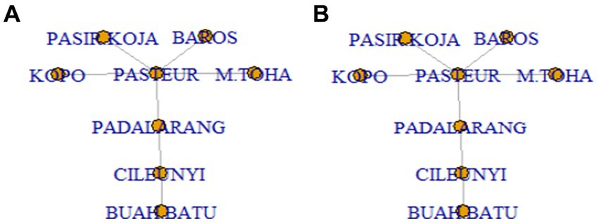
Figure 3. MST in determining: (A) First and (B) Second spatial lag for Pasir Koja. Since Pasteur has a direct line connected to Pasir Koja, it becomes a neighbor in the first lag spatial of Pasir Koja.

2.2 The generalized STAR modeling

The GSTAR model is obtained through Box-Jenkins’ three-stage-iterative model identification, parameter estimation, and diagnostic checking (23). First, all appropriate models can be identified through Space–Time ACF and PACF or named STACF and STPACF. This identification stage has been derived briefly in Pfeifer and Deutsch (35). Then, all possible models may be identified by observing the STACF and STPACF plot pattern, as stated in Table 1.

Table 1

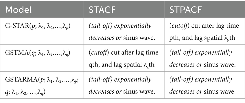
Table 1. STACF and STPACF theoretical patterns in identifying space–time model.

The observation at location $i$ and time $t$ , $Z_i\left(t\right)$ follows the GSTAR model if there is a linear combination of past observations for both time and spatial indices. Suppose, a random vector process { $Z\left(t\right)$ }, $Z\left(t\right)={\left(Z_1\left(t\right),Z_2\left(t\right),\dots ,Z_N\left(t\right)\right)}^{\prime }$ with time $t=\left\{1,2,\dots ,T\right\}$ follows GSTAR $\left(p;{\lambda }_1,{\lambda }_2,\dots ,{\lambda }_p\right)$ model, then $Z\left(t\right)$ can be expressed as follows:

$\begin{array}{ll}Z\left(t\right)={\displaystyle \sum }_{k=1}^p\left[{\Phi }_{k0}Z\left(t-k\right)+{\displaystyle \sum }_{\mathcal{𝓁}=1}^{{\lambda }_k}{\Phi }_{k\mathcal{𝓁}}{\mathbf{W}}^{\left(\mathcal{𝓁}\right)}Z\left(t-k\right)\right]+\epsilon \left(t\right)& (3)\end{array}$

The ${\mathbf{W}}^{\left(\mathcal{𝓁}\right)}$ is $\mathcal{𝓁}$th order weight matrix whose main diagonal is zero and the sum of each row is one, ${\Phi }_{k\mathcal{𝓁}}=\mathit{diag}\left({\varphi }_{k\mathcal{𝓁}}^{\left(1\right)},{\varphi }_{k\mathcal{𝓁}}^{\left(2\right)},\dots ,{\varphi }_{k\mathcal{𝓁}}^{\left(N\right)}\right)$ is (N $\times$ N) diagonal matrix which presents autoregressive parameter of kth time order and $\mathcal{𝓁}$th spatial order for each location $i=1,2,\dots ,N$ , and $\epsilon \left(t\right)=\left({\epsilon }_1\left(t\right),{\epsilon }_2\left(t\right),\dots ,{\epsilon }_N\left(t\right)\right)$ is ( $N\times 1$ )-dimensional vector of errors that is assumed which has i.i.d. normal distribution with null mean and constant variance. Thus, for each location $i=1,2,\dots ,N$ , the model can be written as follows:

$\begin{array}{ll}{Z}_i\left(t\right)={\displaystyle \sum }_{k=1}^p\left[{\varphi }_{k0}^{\left(i\right)}{Z}_i\left(t-k\right)+{\displaystyle \sum }_{\mathcal{𝓁}=1}^{{\lambda }_p}{\varphi }_{k\mathcal{𝓁}}^{\left(i\right)}\left({\displaystyle \sum }_{j=1}^N{w}_{ij}^{\left(\mathcal{𝓁}\right)}{Z}_j\left(t-k\right)\right)\right]+{\epsilon }_i\left(t\right)& (4)\end{array}$

Another important representation of the GSTAR model is the linear model. This form is indispensable when using the least-square (LS) method for parameter estimation. For each location i Equation 4 can be represented by a linear model $Y_i={\mathbf{X}}_i{\varphi }_i+{\epsilon }_i\text{,}$ with $Y_i={\left(Z_i\left(p\right),Z_i\left(p+1\right),\dots ,Z_i\left(T\right)\right)}^{\prime }$, ${\mathbf{X}}_i=\left({\mathbf{U}}_{i1}{\mathbf{U}}_{i2}\cdots {\mathbf{U}}_{im}\right)\text{,}$ ${\varphi }_i={\left({\varphi }_{10}^{\left(i\right)},\dots ,{\varphi }_{1{\lambda }_1}^{\left(i\right)},{\varphi }_{20}^{\left(i\right)},\dots ,{\varphi }_{2{\lambda }_2}^{\left(i\right)},\dots ,{\varphi }_{p0}^{\left(i\right)},\dots ,{\varphi }_{p{\lambda }_p}^{\left(i\right)}\right)}^{\prime }\text{,}$ and ${\epsilon }_i=\left({\epsilon }_i\left(p\right),{\epsilon }_i\left(p+1\right),\dots ,{\epsilon }_i\left(T\right)\right)$. The matrix ${\mathbf{X}}_i$ has size $\left(T-\left(p+1\right)\right)\times \left(p+{\displaystyle \sum }_{m=1}^p{\lambda }_m\right)$, and for $m=1,2,\dots ,p$, defines

${\mathbf{U}}_{im}=\left(\begin{array}{cccc}{Z}_i\left(p-m\right)& {\displaystyle \sum }_{j=1}^N{w}_{ij}^{\left(1\right)}{Z}_j\left(p-m\right)& \cdots & {\displaystyle \sum }_{j=1}^N{w}_{ij}^{\left({\lambda }_m\right)}{Z}_j\left(p-m\right)\\ Z_i\left(p-m+1\right)& {\displaystyle \sum }_{j=1}^N{w}_{ij}^{\left(1\right)}{Z}_j\left(p-m+1\right)& \cdots & {\displaystyle \sum }_{j=1}^N{w}_{ij}^{\left({\lambda }_m\right)}{Z}_j\left(p-m+1\right)\\ ⋮& ⋮& \ddots & ⋮\\ Z_i\left(T-m\right)& {\displaystyle \sum }_{j=1}^N{w}_{ij}^{\left(1\right)}{Z}_j\left(T-m\right)& \cdots & {\displaystyle \sum }_{j=1}^N{w}_{ij}^{\left({\lambda }_m\right)}{Z}_j\left(T-m\right)\end{array}\right)$

The linear model for all locations is defined as $Y=\mathbf{X}\varphi +\epsilon$ , with $Y=\left(Y_1^{\prime },Y_2^{\prime },\dots ,Y_N^{\prime }\right)$ , $\mathbf{X}=\mathit{diag}\left({\mathbf{X}}_1,{\mathbf{X}}_2,\dots ,{\mathbf{X}}_{\mathrm{N}}\right)$ , $\varphi ={\left({\varphi }_1^{\prime },{\varphi }_2^{\prime },\dots ,{\varphi }_N^{\prime }\right)}^{\prime }$ , and $\epsilon ={\left({\epsilon }_1^{\prime },{\epsilon }_2^{\prime },\dots ,{\epsilon }_N^{\prime }\right)}^{\prime }$ . Thus, least-square estimators are obtained by $\hat{\varphi }={\left({\mathbf{X}}^{\mathbf{\prime }}\mathbf{X}\right)}^{-1}{\mathbf{X}}^{\mathbf{\prime }}Y$ .

In the diagnostic checking stage, the error assumption is examined through the normality and uncorrelated test of residuals. The best appropriate model is also obtained by evaluating the model whose residual is minimum. The minimum Akaike information criterion (AIC) and Bayesian information criterion (BIC) may be assessed to choose the best model. Here, the stationarity of the process is reevaluated using parameter estimations to obtain the most appropriate model. Mukhaiyar and Pasaribu (1) introduced the inverse of the autocovariance matrix (IAcM) for evaluating the GSTAR model stationarity through the following propositions.

Proposition 1: Suppose that ( $N\times N$ )-dimensional matrix 𝚨 = 𝚽_𝟏𝟎 + 𝚽_𝟏𝟏𝐖 and IAcM, 𝐌_𝟏 = 𝐈_𝑁 − 𝐀′𝐀, has elements which consist of the parameters of GSTAR(1;1) process, the GSTAR(1;1) model is stationary if the determinants of all the leading principal submatrices of IAcM are positive.

Proposition 2: For GSTAR(1;λ₁) models with λ₁ ≥ 0, define $\mathbf{A}={\displaystyle \sum }_{\mathcal{𝓁}=0}^{{\lambda }_1}{\Phi }_{1\mathcal{𝓁}}{\mathbf{W}}^{\left(\mathcal{𝓁}\right)}$ and IAcM, 𝐌_𝟏 = 𝐈_𝑁 − 𝐀′𝐀, the model is stationary if the determinants of all the leading principal submatrices of M₁ are positive.

Proposition 3: For GSTAR(2; λ₁, λ₂) model, define ${\mathbf{A}}_k={\displaystyle \sum }_{\mathcal{𝓁}=0}^{{\lambda }_k}{\Phi }_{k\mathcal{𝓁}}{\mathbf{W}}^{\left(\mathcal{𝓁}\right)}$ , $k=1,2$ and IAcM, ${\mathbf{M}}_2=\left(\begin{array}{cc}\hfill {\mathbf{I}}_N-{\mathbf{A}}_2^{\prime }{\mathbf{A}}_2\hfill & \hfill -{\mathbf{A}}_1^{\prime }-{\mathbf{A}}_2^{\prime }{\mathbf{A}}_1\hfill \\ \hfill -{\mathbf{A}}_1-{\mathbf{A}}_1^{\prime }{\mathbf{A}}_2\hfill & \hfill {\mathbf{I}}_N-{\mathbf{A}}_2^{\prime }{\mathbf{A}}_2\hfill \end{array}\right)\text{.}$ The models are stationary if the determinants of all the leading principal submatrices of its IAcM are positive.

The proofs of those propositions have been evaluated by Mukhaiyar and Pasaribu (1).

3 Results and discussion

The GSTAR model is obtained through Box-Jenkins’ three-stage-iterative model identification, parameter estimation, and diagnostic checking. First, a weight matrix should be developed; thus, all appropriate models can be investigated through Space–Time ACF and PACF or named STACF and STPACF. Then, since the error assumption is uncorrelated and has constant mean and variance, the ordinary least-square method is applied for parameter estimation.

To get an overview of the GSTAR modeling using the MST weight matrix and its comparison to other approaches, the number of vehicles entering Bandung city through the eight toll gates was investigated. The data retrieved are from January to December 2018, and the plot series and boxplot of each location can be seen in Figure 4. Based on Figure 4, the busiest toll gate is Cileunyi, followed by Pasteur and Padalarang gates. However, some trends are found in some periods (Figure 4A), which means the process is not stationary. Meanwhile, in Figure 4B, some outliers are found in every toll gate, but they will be ignored and still be involved in data analysis. Figure 5 shows the correlation matrix among toll gates observations and its visualization through scatter plots.

Figure 4

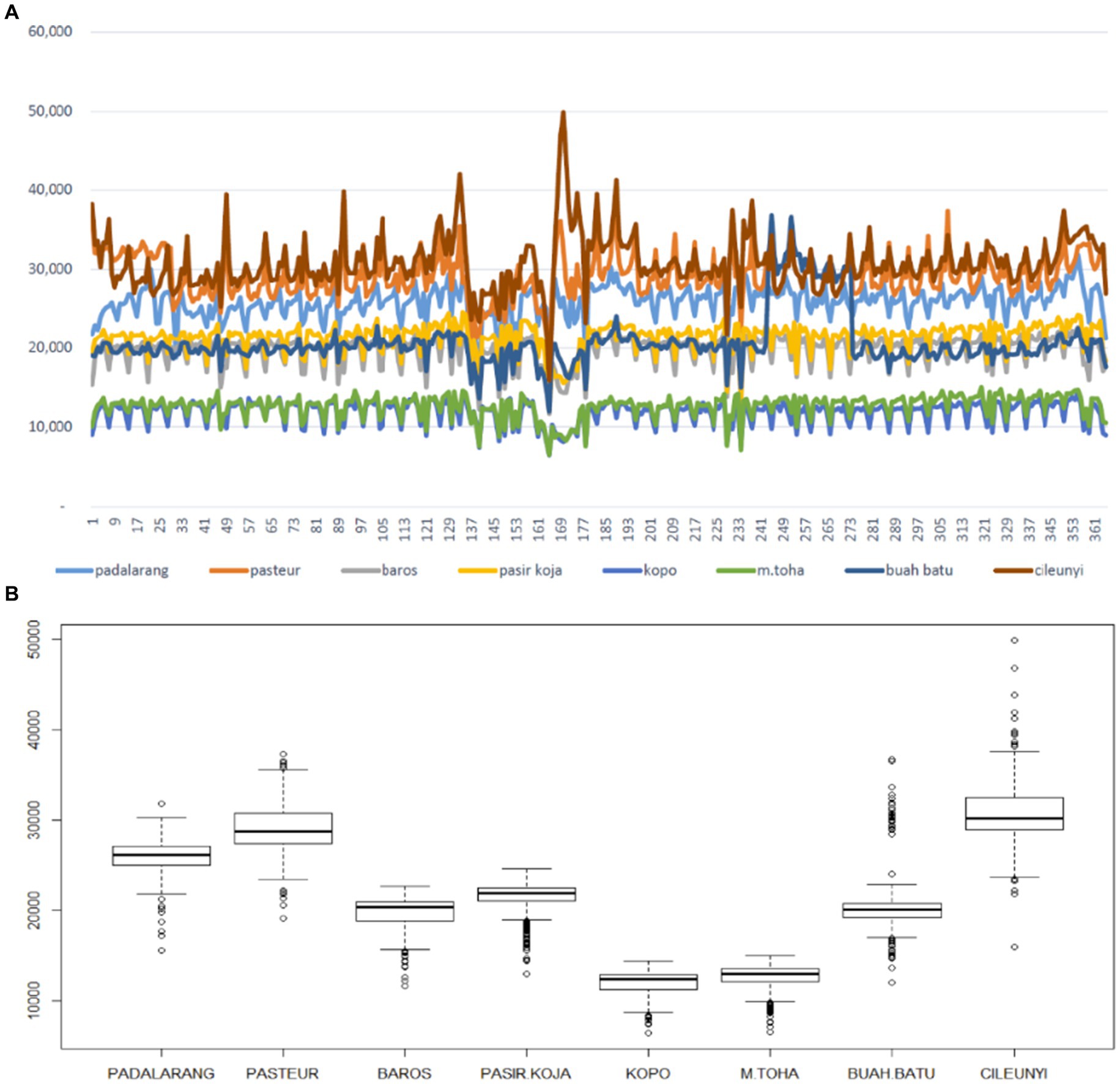
Figure 4. (A) The daily number of vehicles entering Bandung city through eight toll gates. Some trends found in all locations in some periods indicate a non-stationary process. (B) The boxplot for each gate shows the different mean and variability of observations. Some outliers are found in every gate.

Figure 5

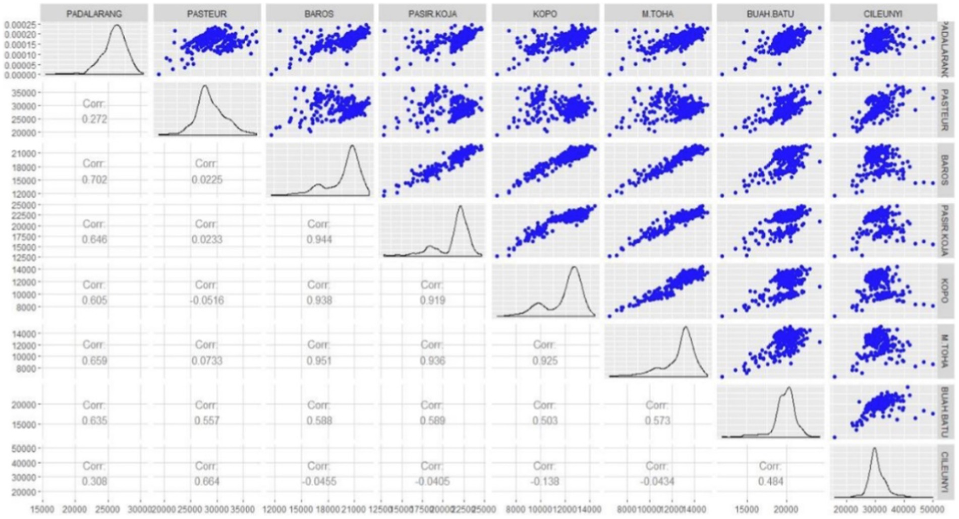
Figure 5. Scatter plot and correlation matrix among toll gate observations.

The highest correlations were obtained among the Baros, Pasir Koja, and Kopo toll gates. These three gates have closer distances in an exact line of the middle toll’s route (see Figure 1). These highest correlations indicate the highest spatial dependencies among other toll gates. It can be seen in the weight matrix (see Table 2). Meanwhile, although Baros’ and Pasteur’s gates are closer, the correlation is the smallest. It is possible since both gates are not in the same line.

Table 2

Table 2. Uniform and inverse distance weight matrix for each approach, radius system, and MST.

The first stage in modeling is identification, in which a plot of STACF and STPACF is performed. To construct both plots, data should be stationary. Then, to make data weak and stationary, differentiation is applied. However, it is not enough, so log transformation is used. Thus, the modeling is carried out to this log-differencing data. After that, a spatial weight matrix should be composed.

There are two types of weight matrices to be applied. Both are uniform and non-uniform (inverse distance), and each type has two approaches, namely, radius system and MST. To build the matrix, the number of neighbors for each location in every spatial lag (there are four spatial lags to be used) must be investigated for each approach as follows:

a. The radius system way needs the distance (mileage) among toll gates and uses a radius (d₀) equal to 10 km (see Figure 2) to obtain the configuration of neighbors.

b. MST way needs a correlation matrix to define the distance matrix based on Equation 3. The distance is the weight in the graph that connects all toll gates. Based on the graph, the MST is obtained every month, and the overall period of observations is consecutively illustrated in Figures 3, 6.

Figure 6

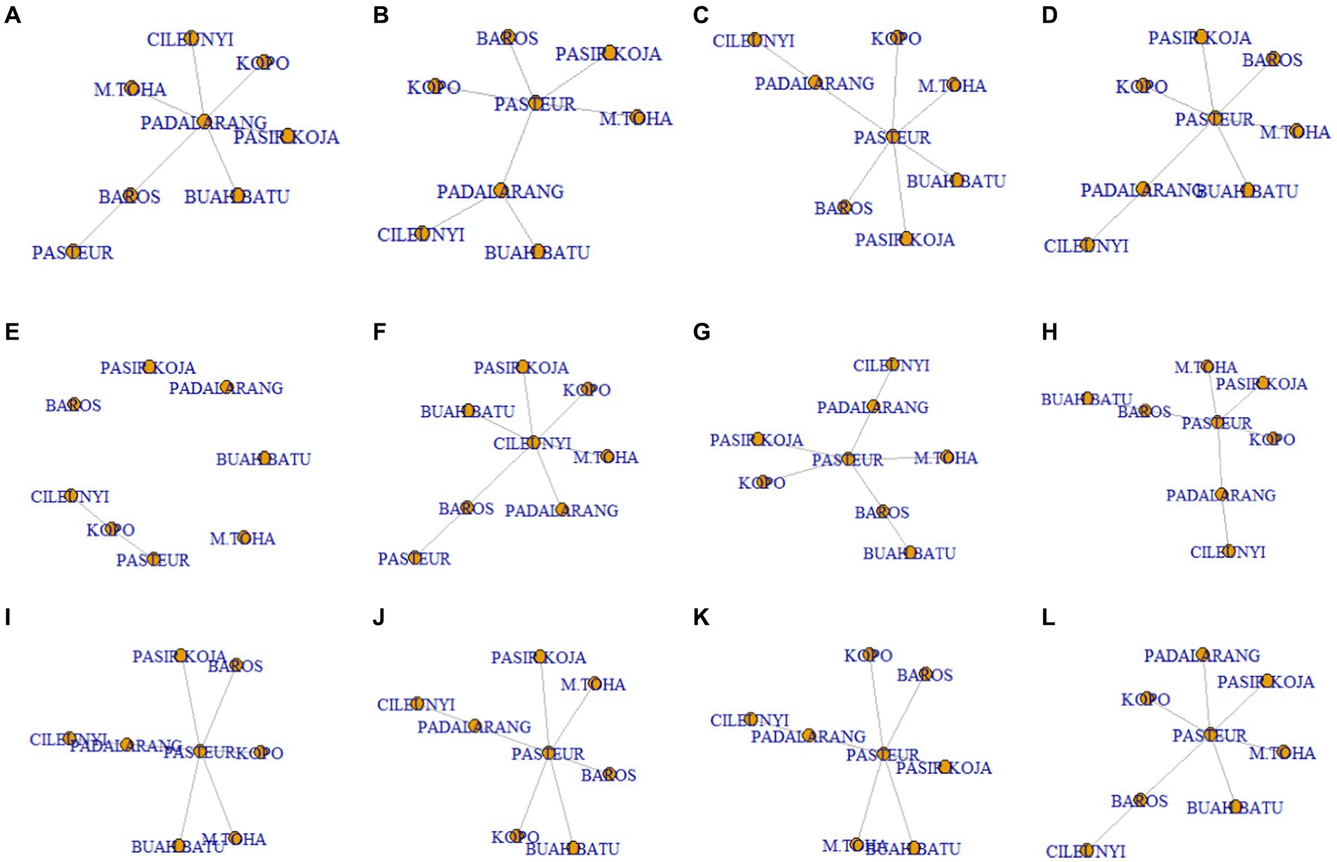
Figure 6. MST was obtained for every month of observations. The Pasteur toll gate is the center of MST most of the time. (A) January. (B) February. (C) March. (D) April. (E) May. (F) June. (G) July. (H) August. (I) September. (J) October. (K) November. (L) December.

The majority of the months have a similar configuration to MST. In contrast, Pasteur toll gate is most frequently the center from February until April and July until December. In addition to the Pasteur toll gate, Padalarang and Cileunyi are also the centers, consecutively in January and June. As a result, those three toll gates are the top three busiest among the observed locations.

The most interesting configuration happened in May, since there are almost no connected graphs among locations, except for Cileunyi, Kopo, and Pasteur, which are connected with a line, and Kopo is the center. It is indicated that the observations’ dependence on toll gates is not significant. There was a long holiday (Eid Al-Fitr celebration) this month, and people simultaneously went in and out of Bandung for homecoming. These observations can also be seen in Figure 4A, during 161–177 days. From both approaches, the configuration of neighbors for every location and spatial lag is obtained as shown in Table 3.

Table 3

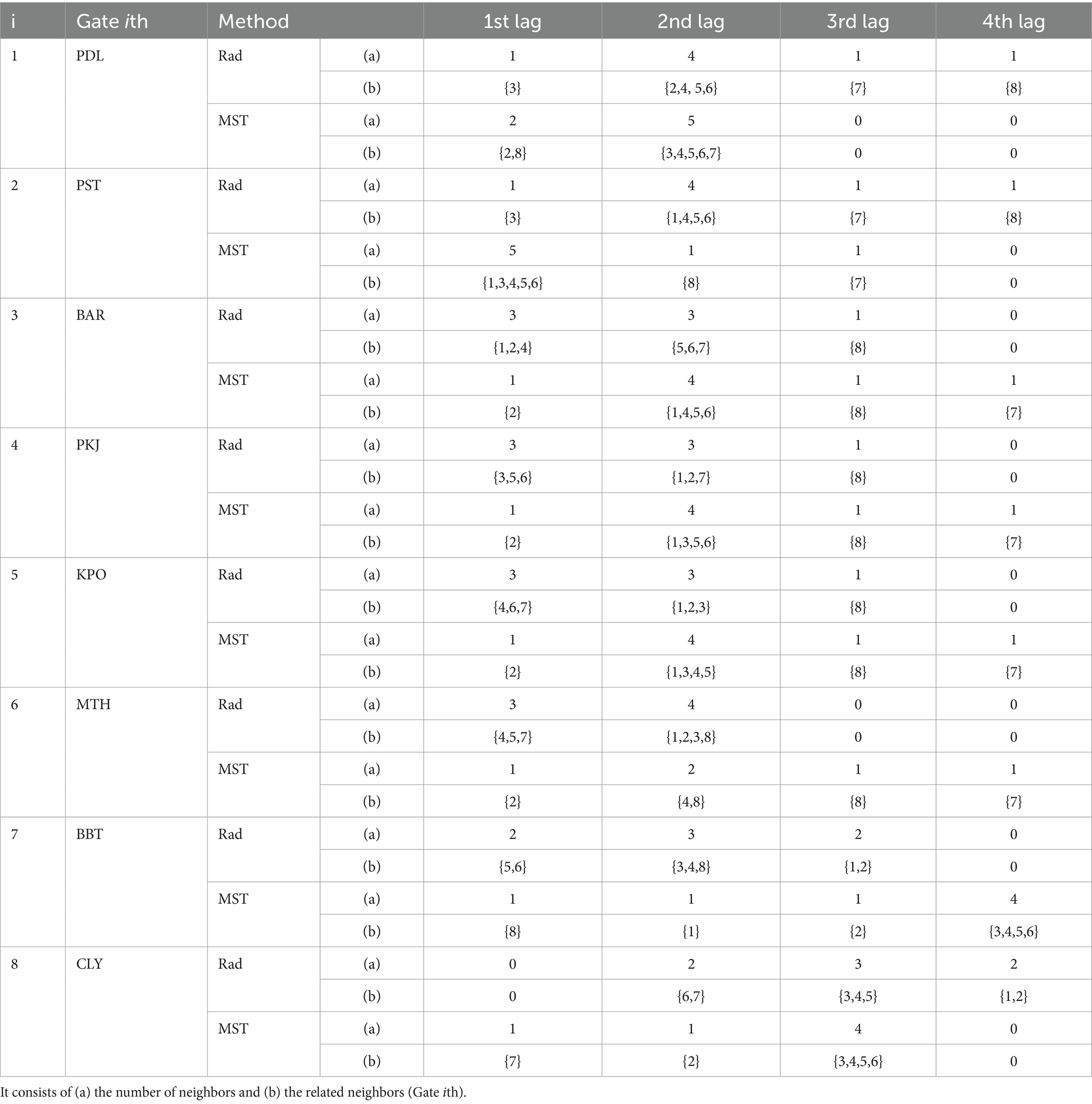
Table 3. Neighbor configuration in every spatial lag using radius system and MST for every location with four different spatial lags.

However, the radius system and the MST approach have different neighbor configurations. For example, as shown in Table 3, the Padalarang gate, using the radius system and MST approach consecutively, has one (3:Baros) and two (2:Pasteur and 8:Cileunyi) neighbors in the first spatial lag and four and five neighbors in the second spatial lag. Meanwhile, in the third and fourth spatial lags, for each, there is only one neighbor obtained using the radius system but no neighbor for the MST approach. Overall, there is a significant difference in the number of neighbors for every spatial lag between the radius system and the MST approach. Therefore, it will have an impact on weight matrix construction.

Based on neighbors’ configurations, the uniform and inverse distance weights are composed using Equations 1, 2. The obtained weight matrices for each spatial lag are concluded in Table 2. It shows a significant difference between the weight matrix’s radius system and the MST approach in line with the configuration.

From the weight matrix, the STACF and STPACF can be calculated. The significance of the autocorrelation is illustrated in Table 4 with symbols “X” for significance and “0” for no significance. Here, the significance value used is 5%. It can be seen from Table 4 that the STACF gives a tail-off pattern because the values are significant for many first lags. Meanwhile, the STACF is cut off in some lags. Therefore, it is indicated that the autoregressive GSTAR model should be considered. Since the pattern of cutoff is quite random, then it is suggested to use the GSTAR model with various simple orders. It is recommended to consider GSTAR(1;1), GSTAR(1,2), and GSTAR(2;1,1) to be involved in the next steps of modeling. After identifying the model, the next step is estimating the model parameters. These parameters were estimated using the least-square method. The estimators were obtained for all parameters of the GSTAR (1; 1), GSTAR (1; 2), and GSTAR (2;1,1) models.

Table 4

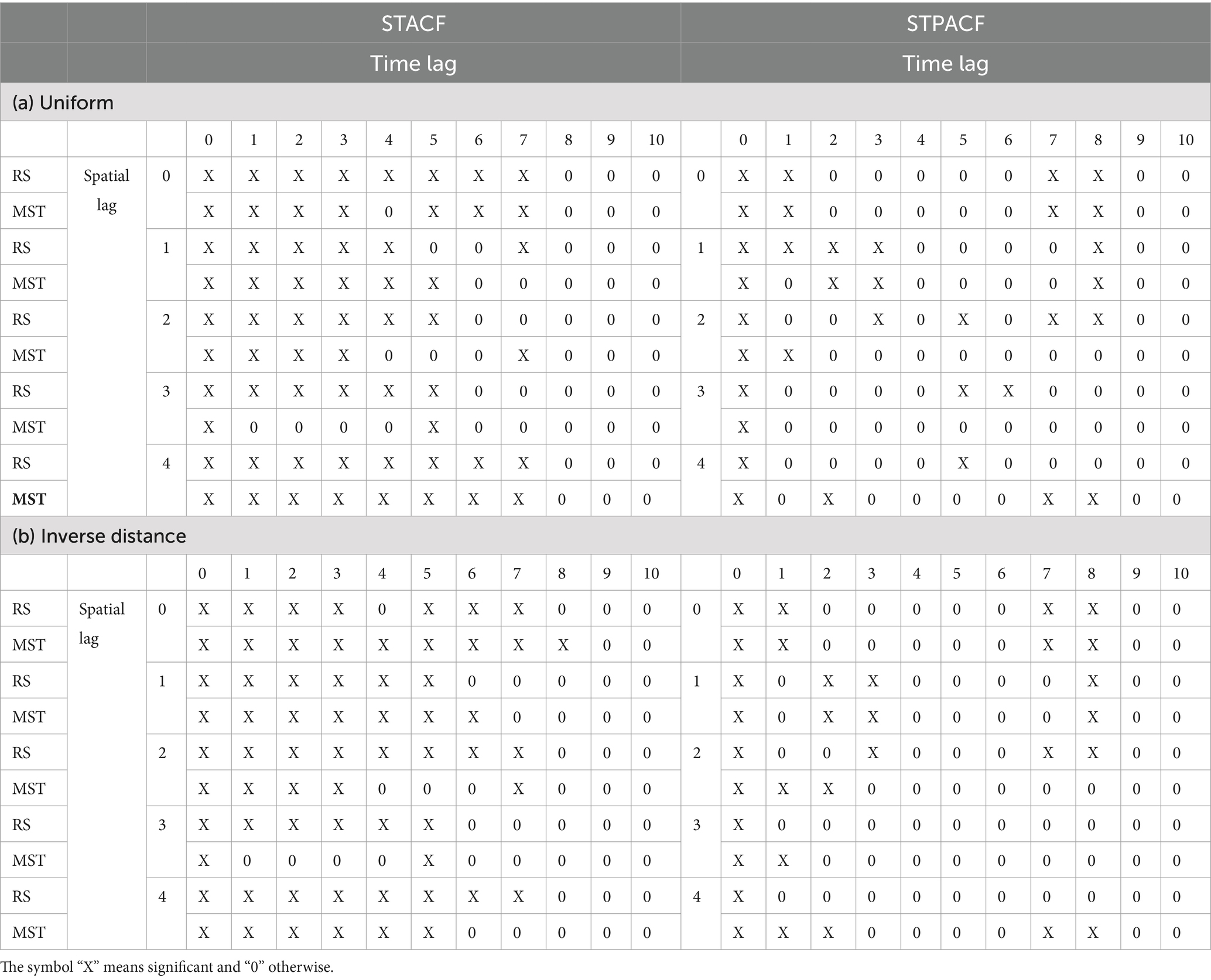
Table 4. STACF and STPACF of weight matrices.

Table 5 shows the parameter estimators using the MST weight matrix. The uniform and inverse distance weight matrix gives similar estimators in some locations, and it depends on the order of the model. It is suspected that larger orders will show less dissimilarity among both types of matrices, especially in a location with low to intermediate variability.

Table 5

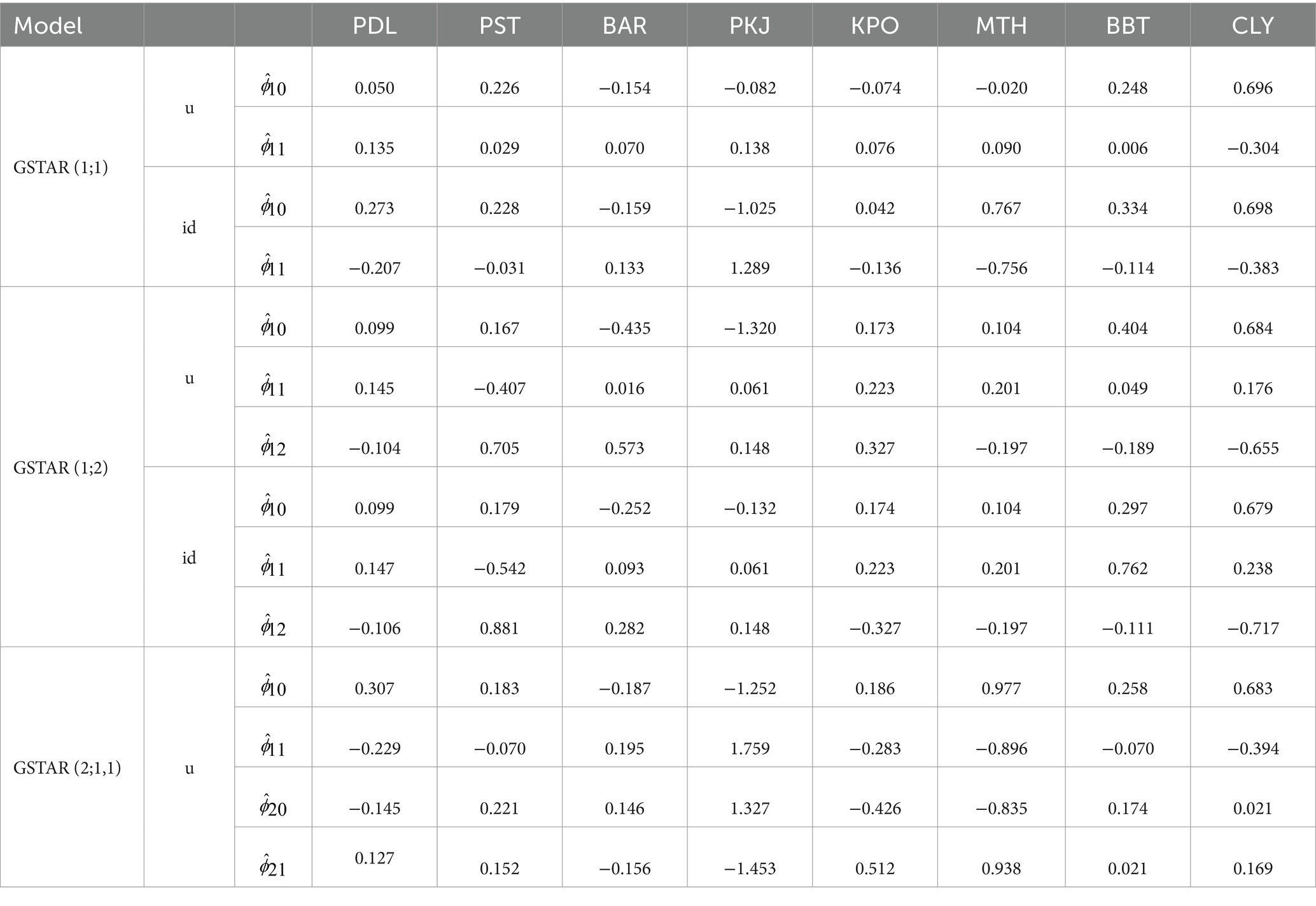
Table 5. Least-square estimators of GSTAR parameters using MST–u (uniform) and MST–id (inverse distance) weight matrix.

After obtaining the estimated parameters, the stationarity of the process can be detected by the inverse of autocovariance matrix (IAcM). This step is part of diagnostic checking. Based on Propositions 1–3, the obtained GSTAR models are stationary since every leading principal submatrix of IAcM has positive determinants. The checklist of this property is summarized in Table 6. The next step is obtaining the least-square estimators.

Table 6

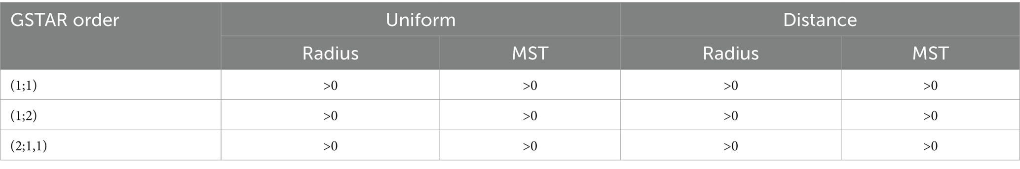
Table 6. Determinant values of leading principal IAcM submatrices show the stationarity of processes.

Consider $z_i$ is the ith real observation of several vehicle numbers and is estimated by ${\hat{z}}_i$ using the obtained models, for $i=1,2,\dots n$ with $n$ as the number of observations, regardless of the time and spatial. Then, the residual is the difference of $z_i$ and ${\hat{z}}_i$ . The residuals are uncorrelated and follow a normal distribution with zero mean and constant variance for a significance value of less than 10%. The best prediction model is obtained by evaluating each model’s root mean square errors (RMSEs) and mean absolute percentage errors (MAPE). First, the RMSE is defined as $\mathit{RMSE}=\sqrt{{\displaystyle \sum }_{i=1}^n{\left(x_i-{\widehat{x}}_i\right)}^2/n}$ . After that, the MAPE is defined as $\mathit{MAPE}=\frac{1}{n}{\displaystyle \sum }_{i=1}^n\left|\frac{Z_i\left(T+1\right)-{\hat{Z}}_i\left(T+1\right)}{Z_i\left(T+1\right)}\right|\times 100\%\text{.}$ The values of RMSE are reported in Table 7.

Table 7

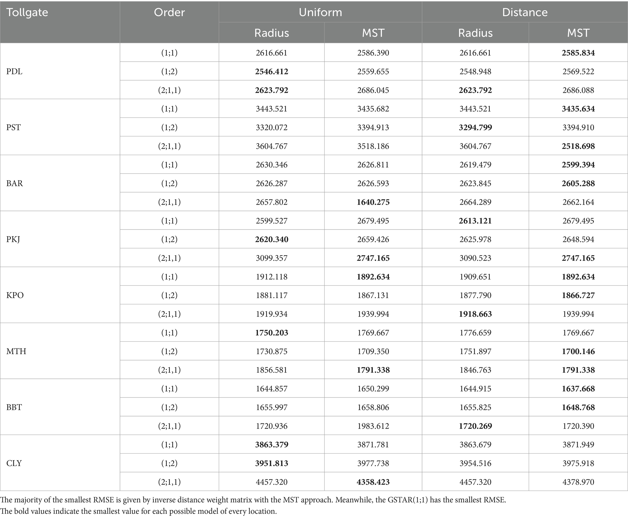
Table 7. RMSE from eight Purbaleunyi toll gates.

It can be seen from Table 7 that the MST inverse distance weight matrix gives the smallest RMSE much more than other types of weight matrices. For example, in the type of model perspective, GSTAR(1;1) has the smallest RMSE values among the obtained models.

The comparison models are also executed for prediction. The observation of $Z_i\left(T+1\right)$ is saved by comparing the one-step prediction result of all models in each location and its MAPE, as shown in Table 8. A slightly different conclusion was obtained from this one-step ahead forecasting. The GSTAR(2;1,1) gives the closest prediction in four (Pasteur, Pasir Koja, Buah Batu, and Cileunyi) of eight toll gates. In Table 8, the MST approach gives the best predictions, especially with the inverse distance approach. Those four toll gates are included in the top five of the busiest toll gates. The GSTAR(1;1) model gives the best prediction in Kopo and M. Toha toll gates using an inverse distance weight matrix.

Table 8

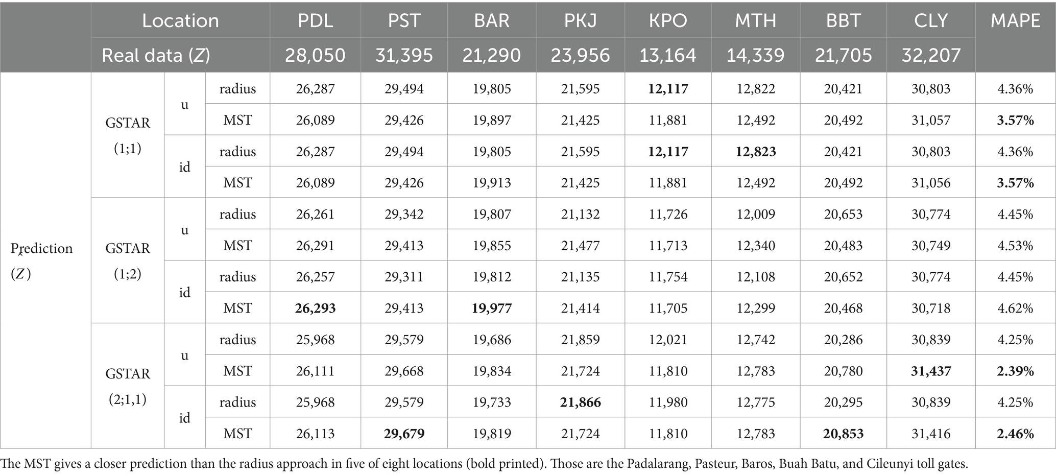
Table 8. Predicted value of the GSTAR model with various weight matrices and its MAPEs.

Overall, the least average of MAPE is presented by GSTAR(2;1,1) with MST, consecutively by uniform (MAPE is 2.39%) and inverse distance approach (MAPE is 2.46%). The next best model is GSTAR(1;1) with MST spatial weight. Both uniform and inverse distance weight matrices give the same MAPE, that is, 3.57. This result aligns with the principle of parsimony in modeling that the model with the least parameters will be better than complex, on condition that the performances are not significantly different for the modeling. Thus, the GSTAR(1;1) with MST inverse distance weight matrix is recommended.

The predicted model using GSTAR(1;1) is formulated as follows:

$\begin{array}{l}{\widehat{Z}}_{\mathrm{P}\mathrm{D}\mathrm{L}}\left(t\right)=0.273Z_{\mathrm{P}\mathrm{D}\mathrm{L}}\left(t-1\right)-0.207\\ \left(0.51Z_{\mathrm{P}\mathrm{S}\mathrm{T}}\left(t-1\right)+\mathbf{0.49}{Z}_{\mathbf{C}\mathbf{L}\mathbf{Y}}\left(t-1\right)\right)\end{array}$

$\begin{array}{l}{\widehat{Z}}_{\mathrm{P}\mathrm{S}\mathrm{T}}\left(t\right)=\mathbf{0.228}{Z}_{\mathbf{P}\mathbf{S}\mathbf{T}}\left(t-1\right)-0.031(0.21Z_{\mathrm{P}\mathrm{D}\mathrm{L}}\left(t-1\right)+0.20\\ Z_{\mathrm{BAR}}\left(t-1\right)+0.20Z_{\mathrm{P}\mathrm{K}\mathrm{J}}\left(t-1\right)+0.19Z_{\mathrm{K}\mathrm{P}\mathrm{O}}\left(t-1\right)\\ +0.20Z_{\mathrm{M}\mathrm{T}\mathrm{H}}\left(t-1\right))\end{array}$

${\widehat{Z}}_{\mathrm{BAR}}\left(t\right)=-\mathbf{0.159}{Z}_{\mathbf{BAR}}\left(t-1\right)+0.133Z_{\mathrm{P}\mathrm{S}\mathrm{T}}\left(t-1\right)$

${\widehat{Z}}_{\mathrm{P}\mathrm{K}\mathrm{J}}\left(t\right)=-1.025Z_{\mathrm{P}\mathrm{K}\mathrm{J}}\left(t-1\right)+\mathbf{1.289}{Z}_{\mathrm{P}\mathrm{S}\mathrm{T}}\left(t-1\right)$

${\widehat{Z}}_{\mathrm{K}\mathrm{P}\mathrm{O}}\left(t\right)=0.042Z_{\mathrm{K}\mathrm{P}\mathrm{O}}\left(t-1\right)-\mathbf{0.136}{Z}_{\mathrm{P}\mathrm{S}\mathrm{T}}\left(t-1\right)$

${\widehat{Z}}_{\mathrm{M}\mathrm{T}\mathrm{H}}\left(t\right)=\mathbf{0.767}{Z}_{\mathrm{M}\mathrm{T}\mathrm{H}}\left(t-1\right)-0.746Z_{\mathrm{P}\mathrm{S}\mathrm{T}}\left(t-1\right)$

${\widehat{Z}}_{\mathrm{B}\mathrm{B}\mathrm{T}}\left(t\right)=\mathbf{0.334}{Z}_{\mathrm{B}\mathrm{B}\mathrm{T}}\left(t-1\right)-0.114Z_{\mathrm{P}\mathrm{S}\mathrm{T}}\left(t-1\right)$

$\begin{array}{l}{\widehat{Z}}_{\mathrm{C}\mathrm{L}\mathrm{Y}}\left(t\right)=\mathbf{0.698}{Z}_{\mathrm{C}\mathrm{L}\mathrm{Y}}\\ \left(t-1\right)-0.383\left(0.43Z_{\mathrm{P}\mathrm{D}\mathrm{L}}\left(t-1\right)+0.57Z_{\mathrm{C}\mathrm{L}\mathrm{Y}}\left(t-1\right)\right)\end{array}$

Based on those equations, every location in a certain time (t) is most influenced by the one previous observation in the same locations, except for Padalarang and Pasir Koja. For both toll gates, consecutively, the previous observation of Cileunyi and Pasteur plays a big role. Different from others, the Baros toll gate has a negative coefficient (−0,159) for its previous observation, which means that the current number of vehicles will decrease linearly to the previous one. With Pasir Koja, Kopo, M. Toha, and Buah Batu, Baros has Pasteur as the only neighbor whose previous observations influenced the respective toll gates. Padalarang, Pasteur, and Cileunyi, the top three busiest toll gates, have their own gates in previous times as the biggest influence on the current observation, except for Padalarang, which has Cileunyi for this case. Pasteur toll gate is influenced by all toll gates, except Buah Batu and Cileunyi toll gates.

The prediction using GSTAR(1;1)–MST inverse distance of weight matrix is plotted in Figure 7. Here, the pattern of re-estimation follows the real observations, although the variability of the estimated observations tends to be smaller than the real observations.

Figure 7

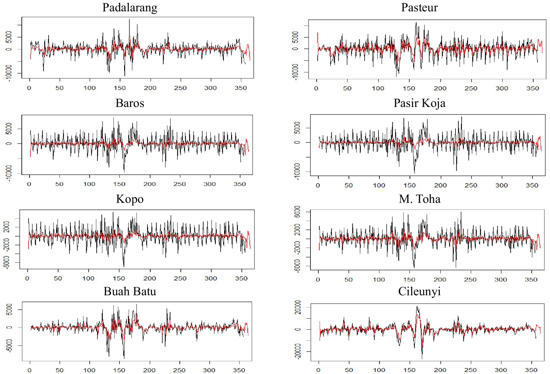
Figure 7. A plot of re-estimation and prediction of observations using the GSTAR(1;1) model with MST inverse distance weight matrix for every toll gate. The real observations (black line) have higher variability than the estimated/predicted observations (red line).

4 Conclusion and remarks

The MST, as a new approach to building the weight matrix of the GSTAR model, can capture the spatial configuration based on space–time observations. This approach is competitive with the conventional approach’s good performance, which is purely based on the inverse distance, in predicting. The MST inverse distance weight matrix is suspected to be appropriate for data with larger variability. The most important thing in building this weight matrix is that the correlation among spatial observations must exist.

Furthermore, since the real observations are the realization of stochastic processes, then the MST approach may give different configurations in different time frames. In this study, the MST approach was built based on all history observations to obtain a fixed weight matrix that can be used to do short-time forecasting. It can be considered as both an advantage and a limitation of this approach. In the future, the weight matrix can be evaluated as a random matrix. It can be the future work of this research.

On the other hand, for the number of vehicles entering Bandung through some toll gates data, the GSTAR(1;1) is the most appropriate to be used. This model is chosen based on the RMSE and AIC-BIC values. Although the prediction result is tight competing with the GSTAR(2;1,1) model, the GSTAR(1;1) is selected due to the parsimony principle in modeling. However, the results of re-estimation and prediction have not been maximal (still not close to the real observations); therefore, the method should be improved. One of the ways to improve is using the SDU approach to obtain a unique MST.

Data availability statement

The raw data supporting the conclusions of this article will be made available by the authors, without undue reservation.

Author contributions

UM: Conceptualization, Data curation, Formal analysis, Funding acquisition, Methodology, Supervision, Validation, Writing – original draft, Writing – review & editing. AM: Supervision, Writing – review & editing. KS: Formal analysis, Supervision, Writing – review & editing. NN: Data curation, Formal analysis, Investigation, Methodology, Resources, Software, Validation, Visualization, Writing – original draft.

Funding

The author(s) declare that financial support was received for the research, authorship, and/or publication of this article. The authors would like to extend their gratitude to the PDUPT research grant of RISTEK-BRIN 2020–2021 (Contract No. 2/E1/KP.PTNBH/2020 and No. 2/E1/KP.PTNBH/2021) for supporting this research and PT. Jasamarga, Purbaleunyi branch for the data. This research is also supported by LPPM ITB through Riset Unggulan ITB 2022 (Contract No. 293/IT1.B07.1/TA.00/2022) and 2024 (Contract No. 959/IT1.B07.1/TA.00/2024).

Conflict of interest

The authors declare that the research was conducted in the absence of any commercial or financial relationships that could be construed as a potential conflict of interest.

Publisher’s note

All claims expressed in this article are solely those of the authors and do not necessarily represent those of their affiliated organizations, or those of the publisher, the editors and the reviewers. Any product that may be evaluated in this article, or claim that may be made by its manufacturer, is not guaranteed or endorsed by the publisher.

References

1. Mukhaiyar, U., and Pasaribu, U. S. The use of IAcM to identify stationarity of the generalized STAR models. (2012) In: 2012 IEEE conference on control, Systems & industrial informatics (pp. 255–260). IEEE.

Google Scholar

2. Yundari, Y., Huda, N. A. M., Pasaribu, U. S., Mukhaiyar, U., and Sari, K. N. Stationary process in GSTAR (1; 1) through kernel function approach. (2020). In: AIP conference proceedings (Vol. 2268, No. 1). AIP Publishing.

Google Scholar

3. Nainggolan, N., and Titaley, J. Development of generalized space time autoregressive (GSTAR) model. (2017). In: AIP conference proceedings (Vol. 1827). AIP Publishing.

Google Scholar

4. Mukhaiyar, U, and Ramadhani, S. The generalized STAR modeling with heteroscedastic effects. CAUCHY J Matematika Murni dan Aplikasi. (2022) 7:158–72. doi: 10.18860/ca.v7i2.13097

Crossref Full Text | Google Scholar

5. Yundari, PUS, Mukhaiyar, U, and Heriawan, MN. Spatial weight determination of GSTAR (1; 1) model by using kernel function. J Phys. (2018) 1028:012223. doi: 10.1088/1742-6596/1028/1/012223

Crossref Full Text | Google Scholar

6. Mukhaiyar, U, Bilad, BI, and Pasaribu, US. The generalized STAR modelling with minimum spanning tree approach of weight matrix for COVID-19 case in Java Island. J Phys. (2021) 2084:012003. doi: 10.1088/1742-6596/2084/1/012003

Crossref Full Text | Google Scholar

7. Masteriana, D., and Mukhaiyar, U. Monte Carlo simulation of error assumptions in generalized STAR (1; 1) model. (2019). In: Proceedings of the Jangjeon Mathematical Society (Vol. 22, pp. 43–50).

Google Scholar

8. Yundari, PUS, and Mukhaiyar, U. Error assumptions on generalized STAR model. J Mathemat Fundamental Sci. (2017) 49:136. doi: 10.5614/j.math.fund.sci.2017.49.2.4

PubMed Abstract | Crossref Full Text | Google Scholar

9. Mukhaiyar, U, Huda, NM, Sari, KN, and Pasaribu, US. Analysis of generalized space time autoregressive with exogenous variable (GSTARX) model with outlier factor. J Phys. (2020) 1496:012004. doi: 10.1088/1742-6596/1496/1/012004

Crossref Full Text | Google Scholar

10. Wardhani, LP, and Kuswanto, H. Poisson GSTAR model: spatial temporal modeling count data follow generalized linear model and count time series models. J Phys. (2020) 1490:012010. doi: 10.1088/1742-6596/1490/1/012010

Crossref Full Text | Google Scholar

11. Gehman, A, and Wei, WW. Optimal spatial aggregation of space–time models and applications. Comput Stat Data Analys. (2020) 145:106913. doi: 10.1016/j.csda.2020.106913

Crossref Full Text | Google Scholar

12. Mukhaiyar, U., Pasaribu, U. S., Budhi, W. S., and Syuhada, K. The stationarity of generalized STAR (2; λ1, λ2) process through the invers of autocovariance matrix. (2014). In: AIP conference proceedings (Vol. 1589, No. 1, pp. 484–487). American Institute of Physics.

Google Scholar

13. Huda, NM, Mukhaiyar, U, and Pasaribu, US. The approximation of GSTAR model for discrete cases through INAR model. J Phys. (2021) 1722:012100. doi: 10.1088/1742-6596/1722/1/012100

Crossref Full Text | Google Scholar

14. Nurhayati, N, Pasaribu, US, and Neswan, O. Application of generalized space-time autoregressive model on GDP data in west European countries. J Probabil Stat. (2012) 2012:1–16. doi: 10.1155/2012/867056

Crossref Full Text | Google Scholar

15. Mukhaiyar, U. The goodness of generalized STAR in spatial dependency observations modeling. (2015). In: AIP conference proceedings (Vol. 1692). AIP Publishing.

Google Scholar

16. Nugraha, R. F., Setiyowati, S., Mukhaiyar, U., and Yuliawati, A. Prediction of oil palm production using the weighted average of fuzzy sets concept approach. (2015). In: AIP conference proceedings (Vol. 1692). AIP Publishing.

Google Scholar

17. Mukhaiyar, U., and Fahmi, F. The generalized STAR (1, 1) modeling with time correlated errors to red-chili weekly prices of some traditional markets in Bandung, West Java. (2015). In: AIP conference proceedings (Vol. 1692). AIP Publishing.

Google Scholar

18. Abdullah, AS, Matoha, S, Lubis, DA, Falah, AN, Jaya, IGNM, Hermawan, E, et al. Implementation of generalized space time autoregressive (GSTAR)-kriging model for predicting rainfall data at unobserved locations in West Java. Appl Maths Informat Sci. (2018) 12:607–15. doi: 10.18576/amis/120316

Crossref Full Text | Google Scholar

19. Mukhaiyar, U, Sari, RKN, and Pasaribu, US. Modeling dengue fever cases by using GSTAR (1; 1) model with outlier factor. J Phys. (2019) 1366:012122. doi: 10.1088/1742-6596/1366/1/012122

Crossref Full Text | Google Scholar

20. Masteriana, D, Riani, MI, and Mukhaiyar, U. Generalized STAR (1; 1) model with outlier-case study of begal in Medan, north Sumatera. J Phys. (2019) 1245:012046. doi: 10.1088/1742-6596/1245/1/012046

Crossref Full Text | Google Scholar

21. Zewdie, MA, Wubit, GG, and Ayele, AW. G-STAR model for forecasting space-time variation of temperature in northern Ethiopia. Turk J Forecast. (2018) 2:9–19. doi: 10.34110/forecasting.437599

Crossref Full Text | Google Scholar

22. Pasaribu, US, Mukhaiyar, U, Huda, NM, Sari, KN, and Indratno, SW. Modelling COVID-19 growth cases of provinces in java island by modified spatial weight matrix GSTAR through railroad passenger's mobility. Heliyon. (2021) 7:e06025. doi: 10.1016/j.heliyon.2021.e06025

PubMed Abstract | Crossref Full Text | Google Scholar

23. Mukhaiyar, U, and Pasaribu, US. A new procedure for generalized STAR modeling using IAcM approach. ITB J Sci. (2012) 44:179–92. doi: 10.5614/itbj.sci.2012.44.2.7

Crossref Full Text | Google Scholar

24. Moretti, F, Pizzuti, S, Panzieri, S, and Annunziato, M. Urban traffic flow forecasting through statistical and neural network bagging ensemble hybrid modeling. Neurocomputing. (2015) 167:3–7. doi: 10.1016/j.neucom.2014.08.100

Crossref Full Text | Google Scholar

25. Giacomazzo, M, and Kamarianakis, Y. Bayesian estimation of subset threshold autoregressions: short-term forecasting of traffic occupancy. J Appl Stat. (2020) 47:2658–89. doi: 10.1080/02664763.2020.1801606

PubMed Abstract | Crossref Full Text | Google Scholar

26. Wang, P, Xu, W, Jin, Y, Wang, J, Li, L, Lu, Q, et al. Forecasting traffic volume at a designated cross-section location on a freeway from large-regional toll collection data. IEEE Access. (2019) 7:9057–70. doi: 10.1109/ACCESS.2018.2890725

Crossref Full Text | Google Scholar

27. Mukhaiyar, U, Nabilah, FT, Pasaribu, US, and Huda, NM. The space-time autoregressive modeling with time correlated errors for the number of vehicles in Purbaleunyi toll gates. J Phys. (2022) 2243:012068. doi: 10.1088/1742-6596/2243/1/012068

Crossref Full Text | Google Scholar

28. Jedwanna, K, Athan, C, and Boonsiripant, S. Estimating toll road travel times using segment-based data imputation. Sustain For. (2023) 15:13042. doi: 10.3390/su151713042

Crossref Full Text | Google Scholar

29. Shi, T, Wang, P, Qi, X, Yang, J, He, R, Yang, J, et al. CPT-DF: congestion prediction on toll-gates using deep learning and fuzzy evaluation for freeway network in China. J Adv Transp. (2023) 2023:1–16. doi: 10.1155/2023/2941035

Crossref Full Text | Google Scholar

30. Niu, J, He, J, Li, Y, and Zhang, S. Highway temporal-spatial traffic flow performance estimation by using gantry toll collection samples: a deep learning method. Math Probl Eng. (2022) 2022:1–10. doi: 10.1155/2022/8711567

Crossref Full Text | Google Scholar

31. Shevchenko, P, Peters, GW, Matsui, T, and Septier, F. Multi-view travel time prediction based on electronic toll collection data. Entropy. (2022) 24:1050. doi: 10.3390/e24081050

Crossref Full Text | Google Scholar

32. Huda, NM, and Imro’ah, N. Determination of the best weight matrix for the generalized space time autoregressive (GSTAR) model in the Covid-19 case on Java Island, Indonesia. Spat Stat. (2023) 54:100734. doi: 10.1016/j.spasta.2023.100734

Crossref Full Text | Google Scholar

33. Bondy, JA, and Murty, USR. Graph theory with applications (Vol. 290). London: Macmillan (1976).

Google Scholar

34. Djauhari, MA, and Gan, SL. Optimality problem of network topology in stocks market analysis. Phys A Stat Mechanics Applic. (2015) 419:108–14. doi: 10.1016/j.physa.2014.09.060

Crossref Full Text | Google Scholar

35. Pfeifer, PE, and Deutsch, SJ. A three-stage iterative approach for space-time modelling. Technometrics. (1980) 22:397–408. doi: 10.1080/00401706.1980.10486172

Crossref Full Text | Google Scholar