Stochastic optimal control problem of consumption and pension insurance with uncertain lifetime and its application to real-life data

We consider a continuous-time model of optimal consumption and pension insurance for a consumer with an uncertain lifetime. In the model, the consumer earns a stochastic wage income during her working life and optimally allocates her income between personal consumption, pension insurance, and securities with a deterministic dynamic return. Due to the weak development of the stock market in developing countries, employees' income comes mainly from wages and interest on savings from banks, that are discussed in this paper. The consumer's utility and bequest functions are constant absolute risk aversion (CARA). By characterizing the optimality condition of the consumer's problem using the Hamilton-Jacobi-Bellman equation, we find the optimal consumption and pension insurance as a function of wealth in closed form. We consider an application of the model while estimating its key elements using real-life data on age-specific population size, labor income, and interest rates. We show that as the absolute risk aversion for consumption increases, consumption and wealth move in the opposite direction. We also present a novel finding that wealth and consumption can be negatively related across consumers with different levels of consumption risk aversion.

1 Introduction

Beginning in the 1960s, numerous researchers have constructed models to analyze the life insurance and the investment behavior of individuals with an uncertain lifetime. Yaari [1] is among the first to explore the life insurance demand in such an environment. Merton [2, 3] developed a continuous time model for optimal consumption and financial investment portfolio. By building on work of Yaari [1] and Merton [2, 3], Richard [4] and Pliska and Ye [5] consider a dynamic programming problem of the life insurance, consumption, and investment of a consumer with an uncertain lifetime. They obtain explicit solutions for the consumer's decision under the constant relative risk aversion (CRRA) utility function. More recent contributions of Chang [6] and Jinchun [7] also consider CRRA utility functions.

The analysis considered in the current paper is closely related to that of Pliska and Ye [8] who analyze a stochastic optimal control problem of consumption, the pension insurance, and investment under an uncertain lifetime. Our work deviates from theirs along three important dimensions. First, unlike the CRRA utility function considered by Pliska and Ye [8], the utility function considered in this paper is CARA (constant absolute risk aversion). Second, in our model, the wage is stochastic throughout the working life of the consumer, which is consistent with data. Third, the hazard function considered in our model is more flexible.

Our specification is highly flexible in the sense that it allows us to capture the shape of the age-specific population size. Specifically, Pliska and Ye [8] model the hazard function as a linear function with two parameters.¹ We specify the hazard function as a piece-wise log quadratic function, with 12 parameters (see Equation 31). The parameters are estimated using the age-specific population size.

Pioneering work of De Moivre [9] modeled the force of mortality as a rational function of age, while Gompertz [10] introduced an exponential model of the force of mortality as a function of age. Makeham [11] extended Gompertz [10] by including age-independent mortality risks. It should be noted that Gompertz [10] and Makeham [11] focus on only adult mortality. Perks [12] modified Gompertz [10] by considering a more flexible logistic mortality. Heligman and Pollard [13] and Thatcher [14] consider a richer setup with eight-parameter logistic mortality that covers the entire age range of the consumer.² In a related setting, Anson [16] specifies the human mortality rate as an age polynomial of degree 5. Over the past 180 years, the earlier models have been applied to data across many countries.

The key advantage of the earlier models is the analytical solution. However, one of the main limitations of these models is their underlying assumption that the population pyramid takes the traditional (expanding) shape. Therefore, these models are not directly applicable to a wide array of countries with declining population growth or a contracting population pyramid.³ To capture more realistic population pyramids, one needs to consider a highly flexible force of mortality. For this reason, we specify the logarithm of the force of mortality as a piecewise smooth continuous function of the third-order B-spline⁴ while using the approach proposed by Oirov [18].

The remainder of the paper is organized as follows. In the Section 2 we present the model, where in the Section 3 we demonstrate the solution of the consumer's problem. Section 4 considers an application of the model to real-life data on the mortality force, the wage process and the interest rate. And finally Section 5 draws the conclusions of the paper.

2 The model

2.1 Setup

Consider a continuous-time economy that consists of three markets: goods, labor and insurance markets. Let t denote the time, where t ∈ R⁺. Consider a consumer who is born at t = 0. Throughout the paper, this consumer will also be referred to as “she” or “the worker,” interchangeably.

The consumer's lifetime, denoted by τ, is a random variable. The maximum age the consumer can reach is T and, therefore, 0 ≤ τ ≤ T. The consumer starts working at time t_w (or, equivalently, at age t_w) and retires at time t_r. The timing of the main life events of the consumer is shown in Figure 1.

Figure 1

Figure 1. Timing of the events.

While employed, the consumer receives the stochastic wage Y(t), t ∈ [t_w, t_r]. The consumer allocates her current income Y(t) among (i) current consumption, (ii) purchasing a pension insurance policy, and (iii) savings. The interest rate on savings is deterministic (i.e. risk-free). The risk-free interest rate is given by the following continuous, smooth function: r(t):R → R⁺.

2.2 The wage process

The wage process $Y(t):\left[t_w,t_r\right]\to R^{+}$ is Borel measurable and satisfies

$\begin{array}{l}{\displaystyle \underset{t_w}{\overset{t_r}{\int }}}E({(Y(t))}^2)dt<\infty .\end{array}$

We suppose that the wage process Y(t) is defined by

$\begin{array}{ll}dY(t)={\mu }_Y(t)dt+{\sigma }_Y(t)dB(t),t_w\le t\le t_r.& (1)\end{array}$

Here, μ_Y(t) is the average wage function, σ_Y(t) is the wage volatility function, and B(t) denotes the Brownian motion.

2.3 Wealth

Let W(t) denote the consumer's wealth at t. At t_w, the consumer is endowed with the initial wealth W_tw. Let c(t) denote the consumption rate, P(t) the amount of insurance purchased, and ϑ(t) the insurance premium rate at time t. Then, the wealth accumulation process can be written as

$\begin{array}{ll}dW(t)=r(t)W(t)dt+dY(t)-c(t)dt-\vartheta (t)P(t)dt,t_w\le t\le t_r.& (2)\end{array}$

2.4 The distribution of the lifetime

Assume that τ is a continuous random variable whose distribution function is F, i.e., F(t) = Pr(τ ≤ t), 0 ≤ t ≤ T. Then, the survival function is S(t) = 1−F(t). Let λ(t) denote the function of the force of mortality, i.e.,

$\begin{array}{l}\lambda (t)=-\frac{S^{\prime }(t)}{S(t)}.\end{array}$

The survival function can be expressed in terms of the force of mortality:

$\begin{array}{l}S(t)=exp\left(-{\displaystyle \underset{0}{\overset{t}{\int }}}\lambda (\xi )d\xi \right).\end{array}$

Then, the cumulative distribution and probability density functions can be written as

$\begin{array}{l}F(t)=1-S(t)=1-exp\left(-{\displaystyle \underset{0}{\overset{t}{\int }}}\lambda (\xi )d\xi \right)\end{array}$

and

$\begin{array}{l}f(t)=\lambda (t)exp\left(-{\displaystyle \underset{0}{\overset{t}{\int }}}\lambda (\xi )d\xi \right).\end{array}$

2.5 Lifetime utility

Let U denote the utility function, where U(c(t)) is the utility drawn from consumption c(t). Also, let Z(τ) be the contingent bequest at the end of the lifetime, while the utility drawn from the bequest is Φ(τ, Z(τ)).

If the consumer's lifetime were deterministic, his or her lifetime utility would be given by

$\begin{array}{l}\psi (\tau )={\displaystyle \underset{0}{\overset{\tau }{\int }}}exp\left\{-{\displaystyle \underset{0}{\overset{t}{\int }}}\rho (\xi )d\xi \right\}U(c(t))dt+\text{Φ}(\tau ,Z(\tau )),\end{array}$

where ρ is the discount rate function, i.e., ρ(t):[0, T] → R⁺. However, since in our model, the lifetime is uncertain, we need to take into account the distribution of the lifetime. Specifically, the expected lifetime utility of the consumer at birth is given by the following weighted integral:

$\begin{array}{l}{E}_f\psi (T)={\displaystyle \underset{0}{\overset{T}{\int }}}\left[{\displaystyle \underset{0}{\overset{t}{\int }}}exp\left(-{\displaystyle \underset{0}{\overset{\omega }{\int }}}\rho (\xi )d\xi \right)U(c(\omega ))d\omega +\text{Φ}(t,Z(t))\right]\text{f(t)}dt.\end{array}$

Using integration by parts, one can obtain the following expected lifetime utility:

$\begin{array}{l}{E}_f\psi (T)={\displaystyle \underset{0}{\overset{T}{\int }}}\left[f(t)\text{Φ}(t,Z(t))+S(t)exp\left(-{\displaystyle \underset{0}{\overset{t}{\int }}}\rho (\xi )d\xi \right)U(c(t))\right]dt.\end{array}$

2.6 The consumer's problem

As stated earlier, t_w is the time at which the consumer starts earning a wage and t_r is the retirement age. That is, the pension insurance payment starts at age t_w and ends at t_r. Therefore, the time period that is relevant for the consumer's problem is t ∈ [t_r, t_w].

Recall that the consumer is endowed with the initial wealth W_tw at age t_w.

$\begin{array}{ll}W(t_w)=W_{t_w}.& (3)\end{array}$

Substituting Equation (2) into Equation (1), the change of wealth is defined by the following equation:

$\begin{array}{ll}dW(t)=(r(t)W(t)+{\mu }_Y(t)-c(t)-\vartheta (t)P(t))dt+{\sigma }_Y(t)dB(t).& (4)\end{array}$

The bequest at t = τ is given by the sum of the wealth and the amount of insurance available at τ:

$\begin{array}{ll}Z(\tau )=W(\tau )+P(\tau ).& (5)\end{array}$

Since consumer's problem covers the period of t ∈ [t_w, t_r], the mortality probability is defined by below conditional probability

$\begin{array}{r}\tilde{f}(t,t_w,t_r)=\frac{f(t)}{F(t_r)-F(t_w)}=\frac{f(t)}{S(t_w)-S(t_r)}\\ \tilde{F}(t,t_w,t_r)=\frac{F(t)-F(t_w)}{F(t_r)-F(t_w)}=\frac{S(t_w)-S(t)}{S(t_w)-S(t_r)}\\ \tilde{S}(t,t_w,t_r)=1-F(t,t_w,t_r)=\frac{S(t)-S(t_r)}{S(t_w)-S(t_r)}\\ \tilde{\lambda }(t,t_w,t_r)=\frac{\tilde{f}(t,t_w,t_r)}{\tilde{S}(t,t_w,t_r)}& (6)\end{array}$

The consumer's problem is given by the following stochastic optimal control problem:

$\begin{array}{ll}{\displaystyle \underset{\left\{c(t),P(t),t_w\to t_r\right\}}{max}}\left\{{\displaystyle \underset{t_w}{\overset{t_r}{\int }}}\left[\tilde{f}(t,t_w,t_r)\text{Φ}(t,Z(t))+\tilde{S}(t,t_w,t)exp\left(-{\displaystyle \underset{t_w}{\overset{t}{\int }}}\rho (\xi )d\xi \right)U(c(t))\right]dt\right\},& (7)\end{array}$

Substituting Equation (6) into Equation (7), the consumer's problem is defined by the following stochastic optimal control problem:

$\begin{array}{l}{\displaystyle \underset{\left\{c(t),P(t),t_w\to t_r\right\}}{max}}\left\{\frac{1}{S(t_w)-S(t_r)}{\displaystyle \underset{t_w}{\overset{t_r}{\int }}}\left[f(t)\text{Φ}(t,Z(t))+(S(t)-S(t_w))exp\left(-{\displaystyle \underset{t_w}{\overset{t}{\int }}}\rho (\xi )d\xi \right)U(c(t))\right]dt\right\},\end{array}$

subject to Equations (3–5).

2.7 Value function

The lifetime utility at age t ∈ [t_w, t_r] is given by the following value function:

$\begin{array}{l}J(t_w,t_r,W(t_w))=\\ {\displaystyle \underset{\left\{c(t),P(t),t_w\to t_r\right\}}{max}}E\{\frac{1}{S(t_w)-S(t_r)}[{\displaystyle \underset{t_w}{\overset{t_r}{\int }}}f(t)\text{Φ}(t,Z(t))\\ +(S(t)-S(t_w))exp\left(-{\displaystyle \underset{t_w}{\overset{t}{\int }}}\rho (\xi )d\xi \right)U(c(t))]dt\},\end{array}$

where t_w ≤ t ≤ t_r. Here, the consumer's wealth increases with the rates of the riskless asset and the wage, but decreases with consumption and the insurance premium. The consumer maximizes the value of the utility function of consumption and bequest,

$\begin{array}{l}J(t_w,t_r,W(t_r))=J_{t_r}=0.\end{array}$

The expected lifetime utility at t > t_w is written as

$\begin{array}{l}J(t,t_r,W(t))=\\ {\displaystyle \underset{\left\{c(t),P(t),t\to t_r\right\}}{max}}E\{\frac{1}{S(t_w)-S(t_r)}{\displaystyle \underset{t}{\overset{t_r}{\int }}}[f(\xi )\text{Φ}(\xi ,Z(\xi ))\\ +(S(\xi )-S(t_w))U(c(\xi ))exp(-{\displaystyle \underset{t_w}{\overset{\xi }{\int }}}\rho (\nu )d\nu )]d\xi \},\end{array}$

where t ≤ ξ ≤ t_r.

3 Solution

We characterize the optimality condition of the consumer's problem specified in the previous section by using the Hamilton-Jacobi-Bellman equation.

3.1 The Hamilton-Jacobi-Bellman equation

Theorem: Suppose that the value function J(t, t_r, W(t)) is of class C². Then J(t, t_r, W(t)) satisfies the Hamilton-Jacobi-Bellman equation

$\begin{array}{c}0={max}_{\left\{c(t),P(t),t\to t_r\right\}}\\ \{[\tilde{\lambda }(t,t_w,t_r)(S(t)-S(t_w))\\ \text{Φ}(t,Z(t))+(S(t)-S(t_w))U(c(t))exp\left({\displaystyle \underset{t_w}{\overset{t}{\int }}}\rho (\xi )d\xi \right)]\\ ·\frac{1}{(S(t_w)-S(t_r))}+[r(t)W(t)+{\mu }_Y(t)-c(t)-\vartheta (t)P(t)]J_W\\ +J_t+\frac{1}{2}{\sigma }_Y^2(t)J_{WW}\}.& (8)\end{array}$

Proof:

$\begin{array}{l}J(t,t_r,W(t))={\displaystyle \underset{\left\{c(t),P(t),t\to t_r\right\}}{max}}E\\ \hspace{1em}\hspace{1em}\hspace{1em}\hspace{1em}\hspace{1em}\hspace{1em}\{\frac{1}{S(t_w)-S(t_r)}{\displaystyle \underset{t}{\overset{t_r}{\int }}}[f(\xi )\text{Φ}(\xi ,Z(\xi ))\\ \hspace{1em}\hspace{1em}\hspace{1em}\hspace{1em}\hspace{1em}\hspace{1em}+(S(\xi )-S(t_w))U(c(\xi ))exp(-{\displaystyle \underset{t_w}{\overset{\xi }{\int }}}\rho (\nu )d\nu )]d\xi \}\\ ={\displaystyle \underset{\{c(t),P(t),t\to t_r\}}{max}}E\{\frac{1}{S(t_w)-S(t_r)}({\displaystyle \underset{t}{\overset{t+\text{Δ}t}{\int }}}[f(\xi )\text{Φ}(\xi ,Z(\xi ))\\ \hspace{1em}\hspace{1em}\hspace{1em}\hspace{1em}\hspace{1em}\hspace{1em}\hspace{1em}+(S(\xi )-S(t_w))U(c(\xi ))exp(-{\displaystyle \underset{t_w}{\overset{\xi }{\int }}}\rho (\nu )d\nu )]d\xi +\\ \hspace{1em}\hspace{1em}\hspace{1em}\hspace{1em}\hspace{1em}\hspace{1em}\hspace{1em}{\displaystyle \underset{t+\text{Δ}t}{\overset{t}{\int }}}[f(\xi )\text{Φ}(\xi ,Z(\xi ))\\ \hspace{1em}\hspace{1em}\hspace{1em}\hspace{1em}\hspace{1em}\hspace{1em}\hspace{1em}+(S(\xi )-S(t_w))U(c(\xi ))exp(-{\displaystyle \underset{t_w}{\overset{\xi }{\int }}}\rho (\nu )d\nu )]d\xi )\}\\ ={\displaystyle \underset{\left\{c(t),P(t),t\to t+\text{Δ}t\right\}}{max}}E\{\frac{1}{S(t_w)-S(t_r)}{\displaystyle \underset{t}{\overset{t+\text{Δ}t}{\int }}}[f(\xi )\text{Φ}(\xi ,Z(\xi ))\\ \hspace{1em}\hspace{1em}\hspace{1em}\hspace{1em}\hspace{1em}\hspace{1em}+(S(\xi )-S(t_w))U(c(\xi ))exp(-{\displaystyle \underset{t_w}{\overset{\xi }{\int }}}\rho (\nu )d\nu )]d\xi \\ \hspace{1em}\hspace{1em}\hspace{1em}\hspace{1em}\hspace{1em}\hspace{1em}+{\displaystyle \underset{\left\{c(t),P(t),t+\text{Δ}t\to t_r\right\}}{max}}\\ \hspace{1em}\hspace{1em}\hspace{1em}\hspace{1em}\hspace{1em}\hspace{1em}E\{\frac{1}{S(t_w)-S(t_r)}{\displaystyle \underset{t+\text{Δ}t}{\overset{t}{\int }}}[f(\xi )\text{Φ}(\xi ,Z(\xi ))\\ \hspace{1em}\hspace{1em}\hspace{1em}\hspace{1em}\hspace{1em}\hspace{1em}+(S(\xi )-S(t_w))U(c(\xi ))exp(-{\displaystyle \underset{t_w}{\overset{\xi }{\int }}}\rho (\nu )d\nu ]d\xi )\}\},& (9)\end{array}$

Using the mean value theorem at the first integral, we get following equation.

$\begin{array}{l}{\displaystyle \underset{t}{\overset{t+\text{Δ}t}{\int }}}[f(\xi )\text{Φ}(\xi ,Z(\xi ))+(S(\xi )-S(t_w))U(c(\xi ))\\ \hspace{1em}\hspace{1em}exp(-{\displaystyle \underset{t_w}{\overset{\xi }{\int }}}\rho (\nu )d\nu )]d\xi \\ \hspace{1em}\hspace{1em}=[f(t+\theta ·\text{Δ}t)\text{Φ}(t+\theta ·\text{Δ}t,Z(t+\theta ·\text{Δ}t))+\\ \hspace{1em}\hspace{1em}(S(t+\theta ·\text{Δ}t)-S(t_w))\\ \hspace{1em}\hspace{1em}·U(c(t+\theta ·\text{Δ}t))exp(-{\displaystyle \underset{t_w}{\overset{t+\theta ·\text{Δ}t}{\int }}}\rho (\nu )d\nu )]·\text{Δ}t\end{array}$

Here, 0 ≤ θ ≤ 1, θΔt ∈ [0, Δt], Δt → 0, follows that

$\begin{array}{l}f(t+\theta \text{Δ}t)·\text{Φ}(t+\theta \text{Δ}t,Z(t+\theta \text{Δ}t))+\\ S(t+\theta \text{Δ}t)-S(t_w))U(c(t+\theta \text{Δ}t))exp(-{\displaystyle \underset{t_w}{\overset{t+\theta \text{Δ}t}{\int }}}\rho (\nu )d\nu )\\ \to f(t)\text{Φ}(t,Z(t))+(S(t)-S(t_w))U(c(t))exp\left(-{\displaystyle \underset{t_w}{\overset{t}{\int }}}\rho (\nu )d\nu \right).\end{array}$

By definition, the second integral is

$\begin{array}{l}{\displaystyle \underset{\left\{c(t),P(t),t+\text{Δ}t\to t_r\right\}}{max}}E\{\frac{1}{S(t_w)-S(t_r)}{\displaystyle \underset{t+\text{Δ}t}{\overset{t}{\int }}}[f(\xi )\text{Φ}(\xi ,Z(\xi ))+\\ (S(\xi )-S(t_w))U(c(\xi ))exp(-{\displaystyle \underset{t_w}{\overset{\xi }{\int }}}\rho (\nu )d\nu )]d\xi \}\\ =J(t+\text{Δ}t,t_r,W(t+\text{Δ}t)).\end{array}$

Now rewriting, Equation (9)

$\begin{array}{r}J\left(t,t_r,W(t)\right)={\displaystyle \underset{\left\{c(t),P(t),t\to t+\text{Δ}t\right\}}{max}}\\ E\{\frac{1}{S(t_w)-S(t_r)}[f(t+\theta \text{Δ}t)\text{Φ}(t+\theta \text{Δ}t,Z(t+\theta \text{Δ}t))+\\ (S(t+\theta \text{Δ}t)-S(t_w))U(c(t+\theta \text{Δ}t))·\\ exp(-{\displaystyle \underset{t_w}{\overset{t+\theta \text{Δ}t}{\int }}}\rho (\nu )d\nu )]\text{Δ}t+J(t+\text{Δ}t,t_r,W(t+\text{Δ}t))\}.\end{array}$

From the last equation, we obtain that

$\begin{array}{l}0={\displaystyle \underset{\{c(t),P(t),t\to t+\text{Δ}t\}}{max}}E\{\frac{1}{S(t_w)-S(t_r)}[f(t+\theta \text{Δ}t)\text{Φ}(t+\theta \text{Δ}t,\\ \hspace{1em}\hspace{1em}Z(t+\theta \text{Δ}t))+(S(t+\theta \text{Δ}t)-S(t_w))\\ \hspace{1em}\hspace{1em}U(c(t+\theta \text{Δ}t))·exp(-{\displaystyle \underset{t_w}{\overset{t+\theta \text{Δ}t}{\int }}}\rho (\nu )d\nu )]\text{Δ}t+\\ \hspace{1em}\hspace{1em}J(t+\text{Δ}t,t_r,W(t+\text{Δ}t))-J(t,t_r,W(t))\}.\end{array}$

Using the Ito's lemma, we obtain that

$\begin{array}{r}J(t+\text{Δ}t,t_r,W(t+\text{Δ}t))-J(t,t_r,W(t))=J_t\text{Δ}t+J_W\text{Δ}W+\\ \frac{1}{2}{J}_{WW}{(\text{Δ}W)}^2+o(\text{Δ}t).\end{array}$

Here, J_t, J_W, J_WW are first and second derivatives from J(t, t_r, W) function. Then, expected value of the Equation (10) is defined by

$\begin{array}{r}E\left\{J(t+\text{Δ}t,t_r,W(t+\text{Δ}t))-J(t,t_r,W(t))\right\}=\\ J_t\text{Δ}t+J_{W}E(\text{Δ}W)+\frac{1}{2}{J}_{WW}E{(\text{Δ}W)}^2+o(\text{Δ}t).& (10)\end{array}$

Here, from Equation (4)

$\begin{array}{l}E(\text{Δ}W)=(r(t)W(t)+{\mu }_Y(t)-c(t)-\vartheta (t)P(t))·\text{Δ}t\\ E{(\text{Δ}W)}^2={\sigma }_Y^2(t)\text{Δ}t& (11)\end{array}$

Substituting Equation (11) into Equation (10), then dividing by Δt and letting Δt go to zero we obtain the Equation (8). Proved theorem.

We choose the value and bequest functions as follows:

$\begin{array}{ll}J(t_w,t,W(t))=exp\left(-{\displaystyle \underset{t_w}{\overset{t}{\int }}}(\rho (\xi )+\tilde{\lambda }(\xi ,t_w,t_r))d\xi \right)V(t,W(t)),& (12)\end{array}$

$\begin{array}{ll}\text{Φ}(t,Z(t))=\frac{1}{\tilde{\lambda }(t,t_w,t_r)}\phi (t,Z(t))exp\left(-{\displaystyle \underset{t_w}{\overset{t}{\int }}}\rho (\xi )d\xi \right),& (13)\end{array}$

where V(·, ·) and φ(·, ·) are the future (time-specific) values associated with J(·, ·) and Φ(·, ·). Substituting Equations (12, 13) into Equation (8), we obtain

$\begin{array}{l}0={\displaystyle \underset{\left\{c(t),P(t)\right\}}{max}}\{\frac{1}{S(t_w)-S(t_r)}\left[\phi (t,Z(t))+U(c(t))\right]-\\ \hspace{1em}\hspace{1em}\hspace{1em}\hspace{1em}\hspace{1em}(\rho (t)+\tilde{\lambda }(t,t_w,t_r))V(t,W(t))+\\ \hspace{1em}\hspace{1em}\hspace{1em}\hspace{1em}\hspace{1em}\left[r(t)W(t)+{\mu }_Y(t)-c(t)-\vartheta (t)P(t)\right]V_W(t,W(t))\\ \hspace{1em}\hspace{1em}\hspace{1em}\hspace{1em}\hspace{1em}+V_t(t,W(t))+\frac{1}{2}{\sigma }_Y^2(t)V_{WW}(t,W(t))\}.& (14)\end{array}$

Then, from Equation (14), the first-order conditions associated with the optimal control problem are derived as

$\begin{array}{ll}\frac{1}{S(t_w)-S(t_r)}{U}_c^{\prime }(c(t))-V_W(t,W(t))=0,& (15)\end{array}$

$\begin{array}{ll}\frac{1}{S(t_w)-S(t_r)}{\phi }_Z^{\prime }(t,Z(t))-\vartheta (t)V_W(t,W(t))=0,& (16)\end{array}$

where t_w ≤ t ≤ t_r.

3.2 The utility and bequest functions

Let us choose the following forms of the utility function of consumption and bequest:

$\begin{array}{ll}U(c(t))=-\frac{\alpha }{\beta }exp\left\{-\beta ·c(t)\right\},& (17)\end{array}$

$\begin{array}{ll}\phi (t,Z(t))=-\frac{A(t)}{k}exp\left\{-k·Z(t)\right\},& (18)\end{array}$

where the parameters α, β, k are all greater than zero, and the functions A(·) and Z(·) are yet to be determined.

In Equations (17, 18), the two key parameters are β and k, which denote, respectively, the absolute risk aversion coefficients of the utility and bequest functions. Below, in the numerical application, we will focus on the impact of these two risk aversion coefficients, i.e., on the impact of parameters β and k.

Given the specifications in Equations (17, 18), the value function takes the following form:

$\begin{array}{ll}V(t,W(t))=-\frac{b(t)}{a(t)}exp\left\{-a(t)W(t)\right\}.& (19)\end{array}$

In Equation (19), the two functions, a(·) and b(·), fully determine how the value function depends on wealth. The positive deterministic function a(·) captures the extent of the relative risk aversion of the value function. The function b(·) is also positive and deterministic. However, the coefficients of b(·) are allowed to be time-varying. Below, in our numerical implementation below, we determine these functions using the method of undetermined coefficients.

Let's define the optimal consumption and premium as a function of u(t, c(t)) and φ(t, Z(t)). By using the first-order condition in Equation (15), we have the following optimal consumption function:

$\begin{array}{ll}{c}^{*}(t)=\frac{1}{\beta }\left\{a(t)W(t)-ln\left[\frac{b(t)(S(t_w)-S(t_r))}{\alpha }\right]\right\}.& (20)\end{array}$

Furthermore, by applying the first-order condition in Equation (16), we have

$\begin{array}{ll}A(t)=\vartheta (t)b(t)(S(t_w)-S(t_r)),& (21)\end{array}$

$\begin{array}{ll}{P}^{*}(t)=\left(\frac{a(t)}{k}-1\right)W(t).& (22)\end{array}$

By substituting Equations (20–22), V_t, V_W and V_WW into Equation (14), the Hamilton-Jacobi-Belman equation is simplified to

$\begin{array}{l}0=-\frac{\vartheta (t)b(t)}{k}-\frac{b(t)}{\beta }+(\rho (t)+\tilde{\lambda }(t,t_w,t_r))\frac{b(t)}{a(t)}-\frac{b^{\prime }(t)}{a(t)}+\\ \hspace{1em}\hspace{1em}\frac{b(t)a^{\prime }(t)}{a^2(t)}+\frac{b(t)a^{\prime }(t)}{a(t)}W(t)+r(t)b(t)W(t)+{\mu }_Y(t)b(t)-\\ \hspace{1em}\hspace{1em}\frac{a(t)b(t)}{\beta }W(t)+\frac{b(t)}{\beta }ln\left[\frac{b(t)(S(t_w)-S(t_r))}{\alpha }\right]-\\ \hspace{1em}\hspace{1em}\frac{\vartheta (t)a(t)b(t)}{k}W(t)+\vartheta (t)b(t)W(t)-\frac{1}{2}{\sigma }_Y^2(t)a(t)b(t).\end{array}$

Hence we can find the Bernoulli equation for a(t) as

$\begin{array}{ll}{a}^{\prime }(t)+(r(t)+\vartheta (t))a(t)=\left(\frac{1}{\beta }+\frac{\vartheta (t)}{k}\right)a^2(t).& (23)\end{array}$

It follows that

$\begin{array}{l}a(t)=[exp\left({\displaystyle \underset{t_r}{\overset{t}{\int }}}(r(\xi )+\vartheta (\xi ))d\xi \right)\times \\ \{cons{t}_a-{\displaystyle \underset{t_r}{\overset{t}{\int }}}\left(\frac{1}{\beta }+\frac{\vartheta (\xi )}{k}\right)exp\left(-{\displaystyle \underset{t_r}{\overset{\xi }{\int }}}(r(\eta )+\vartheta (\eta ))d\eta \right)d\xi \}{]}^{-1}\end{array}$

and

$\begin{array}{ll}{\left[lnb(t)\right]}^{\prime }-\frac{a(t)}{\beta }lnb(t)=D(t),& (24)\end{array}$

where

$\begin{array}{r}D(t)={\rho }^{*}(t)-r(t)-\vartheta (t)+{\mu }_Y(t)a(t)-\frac{1}{2}{\sigma }_Y^2(t)a^2(t)+\\ \frac{a(t)}{\beta }ln\left(\frac{S(t_w)-S(t_r)}{\alpha }\right),& (25)\end{array}$

$\begin{array}{ll}{\rho }^{*}(t)=\rho (t)+\tilde{\lambda }(t,t_w,t_r).& (26)\end{array}$

Here, ρ^*(t) is the effective discount rate associated with the nominal lifetime utility value of time t (also, see Equation 12).

Since Equation (24) is a linear differential equation, its solution can be found as

$\begin{array}{l}b(t)=exp\{exp\left({\displaystyle \underset{t_r}{\overset{t}{\int }}}\frac{a(\xi )}{\beta }d\xi \right)\\ \hspace{1em}\hspace{1em}\hspace{1em}\hspace{1em}\times (cons{t}_b+{\displaystyle \underset{t_r}{\overset{t}{\int }}}D(\xi )(exp(-{\displaystyle \underset{t_r}{\overset{\xi }{\int }}}\frac{a(\eta )}{\beta }d\eta ))d\xi )\}.\end{array}$

From Equations (20, 22), it can be seen that the extent to which the optimal consumption and the optimal insurance amount depend on wealth is influenced by the function a(·). As with any dynamic programming problem, the consumer's current decision amounts to maximizing the value function associated with the remaining lifetime. Furthermore, the key element driving the risk aversion of the value function is the risk aversion coefficient of the bequest function. Given these considerations, we make the following assumption:

$\begin{array}{ll}a(t)=k\xi (t)\text{for all }t.& (27)\end{array}$

Under such a specification, the function ξ(·) can be retrieved from Equation (23). Inserting Equation (27) into Equation (23), one can obtain the following so-called Bernoulli's equation:

$\begin{array}{ll}{\xi }^{\prime }(t)+(r(t)+\vartheta (t))\xi (t)=\left(\frac{k}{\beta }+\vartheta (t)\right){\xi }^2(t).& (28)\end{array}$

The solution of Equation (28) is given by

$\begin{array}{ll}{c}^{*}(t)=\frac{1}{\beta }\left(k\xi (t)W(t)-ln(\frac{b(t)}{\alpha })\right),& (29)\end{array}$

$\begin{array}{ll}P(t)=(\xi (t)-1)W(t).& (30)\end{array}$

For the type of analyses such as ours, one of the most frequent assumptions in the literature is the constant relative risk aversion (CRRA). Consistently, we also consider the CRRA for both the utility and bequest functions. This specification allows us to solve the stochastic optimization problem specified in Section (2.6) analytically.

Equations (29, 30) imply that the optimal consumption level and optimal insurance amount are both linear in wealth. Moreover, the slope of the optimal consumption as a function of wealth depends on one the ratio of the two RRA coefficients k/β. These results are in line with those obtained by Richard [4] using CRRA functions.

However, our analysis differs from the existing literature in one important way. The earlier studies are usually concerned with obtaining an analytical solution and drawing general conclusions from the analytical solution. Our analysis goes a step further. Specifically, using the analytical solution, we conduct a set of numerical experiments and have a deeper look into the impact of the risk aversion parameters.

3.3 Difference scheme

Using the difference scheme, the Equations (24, 25, 28) can be written in the discrete-time setting as follows:

$\begin{array}{l}b(t+1)=b(t)\left[1+\frac{k\xi (t)}{\beta }ln(b(t))+D(t)\right],\\ D(t)={\rho }^{*}(t)-r(t)-\vartheta (t)+({\mu }_Y(t)+\frac{1}{\beta }ln\left(\frac{S(t_w)-S(t_r)}{\alpha }\right))\\ k\xi (t)-\frac{{\sigma }_Y^2(t)k^2{\xi }^2(t)}{2},\end{array}$

$\begin{array}{l}\xi (t+1)=(1-r(t)-\vartheta (t))\xi (t)+\left(\frac{k}{\beta }+\vartheta (t)\right){\xi }^2(t).\end{array}$

4 Application

As an important contribution of our analysis to the current literature, we apply the model to real-life data and examine both the qualitative and quantitative effects of the parameters. For this purpose, we need to construct deterministic functions such as the mortality force, the wage process, and the interest rate. We estimate these functions using data on aggregate and age-specific data from Mongolia. The data used in our estimation are available from the Mongolbank (the central bank of Mongolia) and the National Statistical Office (NSO) of Mongolia.

As with many post-communist countries, Mongolia's population pyramid had experienced dramatic changes during its transition period, which lasted throughout the 1990s and early 2000s. Consequently, the age distribution of the population can not be adequately captured by standard distributions. We overcome this challenge by using the piece-wise cubic spline method developed by Oirov [18].

4.1 B-spline functions

Consider a set of nth order B-spline functions defined on a set of knots q_{k, n} = (q₁, q₂, …, q_2n+k). Suppose that the knots are set up in the following manner:

$\begin{array}{r}\eta =q_1=q_2=\dots =q_n<q_{n+1}<\dots <q_{n+k}<q_{n+k+1}=\\ \dots =q_{2n+k}=\zeta ,\end{array}$

where 0 ≤ η < ζ < ∞.

Also, let

$\begin{array}{l}{G}_k=\left\{g(t,\theta ,{\text{q}}_{k,n}):\theta \in {ℝ}^{n+k},{\text{q}}_{k,n}\in {ℝ}^{2n+k}\right\}.\end{array}$

The B-splines are defined on the set through the following recurence relation:

$\begin{array}{l}g(t;\theta ,{\text{q}}_{k,n})={\displaystyle \sum _{j=1}^p}{\theta }_j{B}_{j,n}(t,{\text{q}}_{k,n}),\end{array}$

where ⊺ denotes the transpose of a matrix.

One can specify λ(t) = g(t, θ, q_{k, n}). However, such a specification will complicate the analysis by imposing an additional constraint that g(t; θ, q_{k, n}) > 0 for all t. We consider an alternative specification where no such additional constraint is required. Specifically, we set

$\begin{array}{l}ln(\lambda (t))=g(t;\theta ,{\text{q}}_{k,n}).\end{array}$

4.2 Estimation of force of mortality

To estimate the logarithm of the force of mortality, we use a third-order B-spline function. We determine the B-spline parameters using maximum likelihood estimation, where the criterion is the modified chi-squared goodness of the fit statistic. In doing so, we develop an algorithm for the Sequential Procedure of the modified chi-squared goodness of the fit testing. In our estimation, we assume that T, the maximum age, is 100 years.

The estimation based on the 2019 Mongolian population data yields the following logarithm of the force of mortality:

$\begin{array}{ll}\begin{array}{l}\ln (\lambda (t))=\{\begin{array}{cc}+2.355\times {10}^{-3}{t}^2-0.066t-3.346,& 0\le t<30;\\ +0.070\times {10}^{-3}{t}^2-12.797t-3.049,& 30\le t<59;\\ -9.300\times {10}^{-3}{t}^2+3.398t+179.514,& 59\le t<62;\\ +1.800\times {10}^{-3}{t}^2-0.234t+5.457,& 62\le t\le 100.\end{array}\hfill \end{array}& (31)\end{array}$

The Figure 2 depicts the estimated function by a red solid line. In the figure, the empirical values are depicted by the blue stars. Using the estimated force of mortality, we find the survival and density functions.

Figure 2

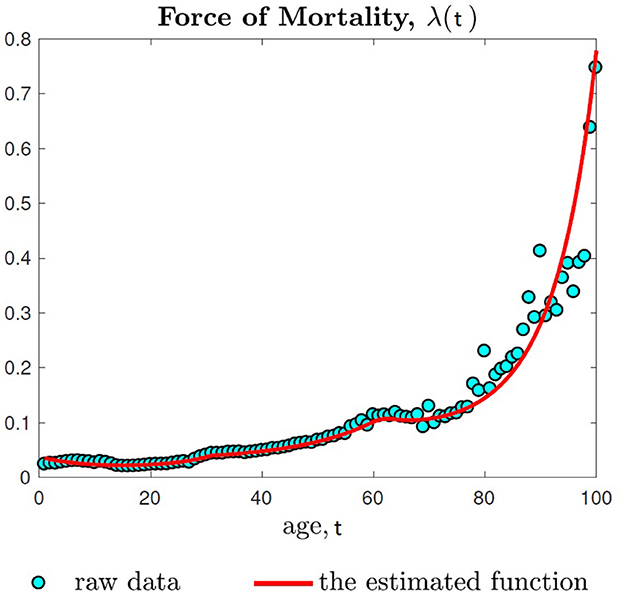
Figure 2. The estimation is based on the 2019 age-specific population available from the NSO of Mongolia. See Equation (31) for further details.

4.3 The interest rate and wage functions

The interest rate function r(·) is estimated by using the annual savings rates of 2008–2021 tabulated by Mongolbank at By fitting the savings rates to a linear trend, we obtain the following function for the interest rate:

$\begin{array}{l}r(t)=0.1-0.002(t-t_w).\end{array}$

Our simulation assumes that the consumer begins to purchase the insurance policy at age t_w = 25 and retires at age t_r = 60. The average wage function μ_Y(·) and the wage volatility function σ_Y(·) are estimated using real average wage series from 1995-2020, which is available from the NSO.We fit the age-specific average annual wages to a linear trend. Our empirical analysis shows that the average wage function exhibits strong monotonicity while the wage volatility function is virtually constant. Specifically, we obtain the following estimates for the wage process:

$\begin{array}{ll}\{\begin{array}{l}{\mu }_Y(t)=0.22+0.11(t-t_w),\\ {\sigma }_Y(t)=0.21,\end{array}& (32)\end{array}$

where 25 = t_w ≤ t ≤ t_r = 60. The simulated wage process used in our application is illustrated in Figure 3.

Figure 3

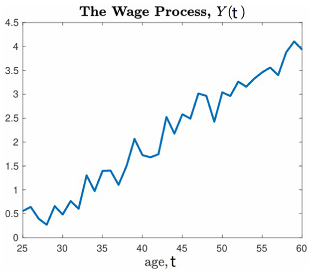
Figure 3. The figure shows the wage process that is simulated using Equation (1) and estimates in Equation (32). The vertical axis is in million units of the national currency, tugriks.

4.4 Discount and insurance premium rates

Our empirical analysis reveals that in Mongolia, the force of mortality for those aged 60 is ~0.11. Based on this number, we set ρ^*(t) = 0.15 for all t. Then, using Equation (26), the discount rate becomes

$\begin{array}{l}\rho (t)=0.15-\hat{\lambda }(t,t_w,t_r),\end{array}$

where $\hat{\lambda }(t,t_w,t_r)$ is given by Equation (31). Furthermore, for the insurance premium rate, we adopt the following specification from Richard [4]:

$\begin{array}{l}\vartheta (t)=\hat{\lambda }(t,t_w,t_r)+\frac{0.9}{t}.\end{array}$

4.5 The parameter values

Given the estimated functions, we conduct a set of numerical experiments by assuming specific values for the remaining parameters.

The values of β considered in our analysis are guided by the extensive empirical literature on relative risk aversion. Brown [19] argues that the RRA coefficient ranges between 0.5 and 3.0, depending on an individual's age and occupation. Gourinchas and Parker [20] and Lin [21] report slightly wider ranges: the range of the RRA coefficient in Gourinchas and Parker [20] is 0.15–5.30, while that in Lin [21] is 0.8–5.3.⁵ It is from these ranges that the values of the relative risk aversion coefficient of the utility function are chosen. Specifically, in our numerical experiments, we consider two values of β: 0.5 and 1.0.

We consider two values of the ARA coefficient for the bequest function: 0.01 and 0.02. These values guarantee plausible differences in consumption and pension insurance between different types of consumers considered in the analysis.

4.6 Consumer types

In our analysis, we consider three types of consumers referred to as

(i) the consumer with high ARA for bequest (hereafter the high ARAB consumer);

(ii) the median consumer; and

(iii) the consumer with high ARA for consumption (hereafter the high ARAC consumer).

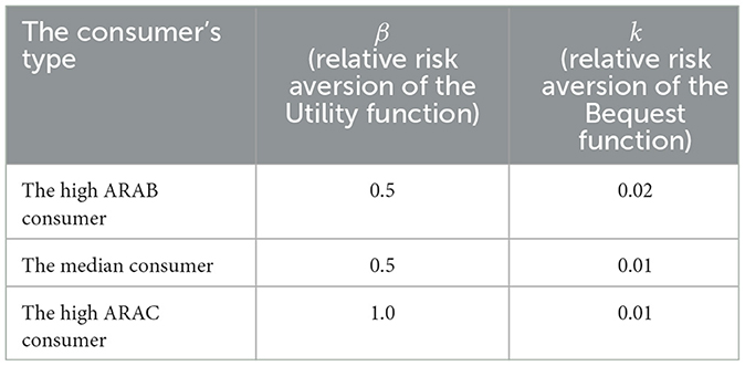
The ARA parameters of their utility and bequest functions are shown in Table 1.

Table 1

Table 1. Key parameters of the utility and bequest functions.

The difference between the median and high ARAB consumers is that the ARA parameter k of the bequest function is higher for the high ARAB consumer. That is, compared to the median consumer, the high ARAB consumer is more averse to the volatility of the bequest. The difference between the median and high ARAC consumers is that the ARA parameter β of the utility function is higher for the high ARAC consumer. In other words, compared to the median consumer, the high ARAC consumer is more averse to the volatility of her own consumption.

4.7 Simulation results

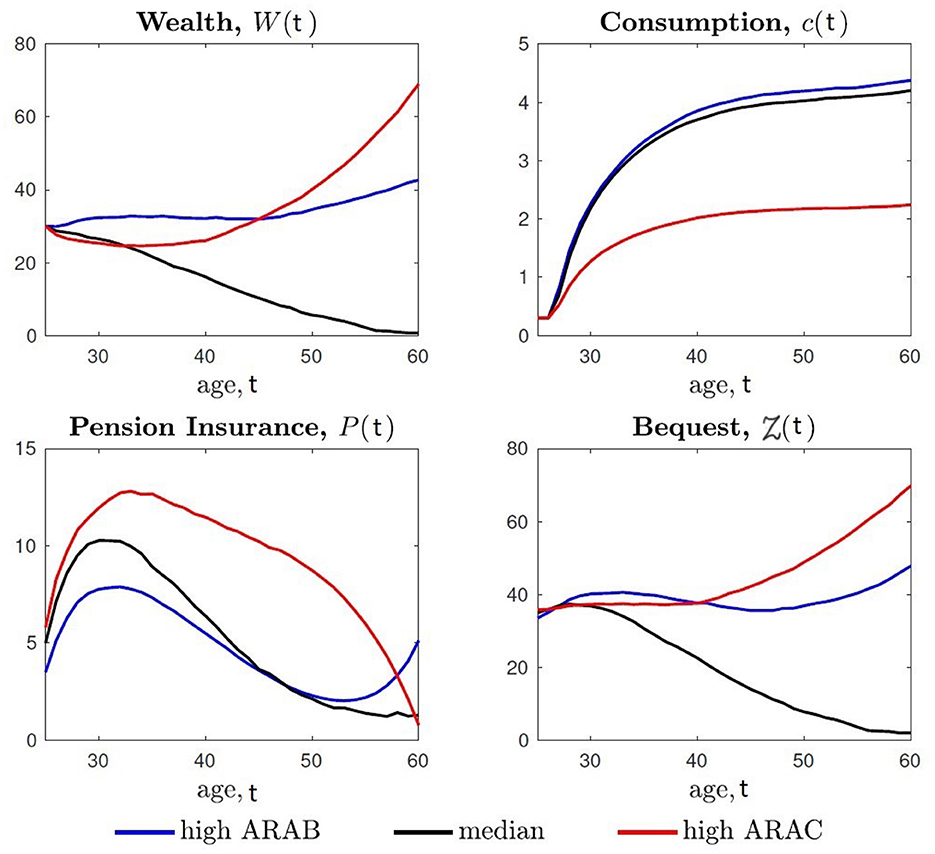
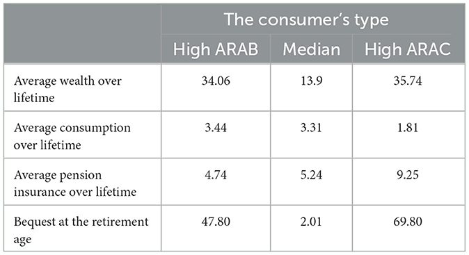
Figure 4 displays the age-specific wealth, consumption, the pension insurance and the bequest of the three consumers. Table 2 summarizes the overall level of wealth, consumption and the pension insurance, as well as the amount of bequest at the retirement age.

Figure 4

Figure 4. Wealth, consumption, pension insurance, and bequest by age.

Table 2

Table 2. Wealth, consumption, pension insurance, and bequest.

Despite the same income process, the same mortality risk, and the same interest rate, the high ARAC consumer has substantially lower consumption. This happens because of her higher absolute risk aversion for consumption: a marginal increase in consumption has a stronger negative impact on her marginal utility of consumption.

The high ARAC consumer's absolute risk aversion (ARA) for the bequest is much lower than her ARA for consumption. In other words, an increase in the bequest has a lower negative effect on her marginal utility than an increase in consumption. Therefore, the high ARAC consumer has the highest average wealth and pension insurance over her lifetime.

Analogously, the high ARAB consumer's absolute risk aversion (ARA) for consumption is lower than her ARA for the bequest. Consequently, the high ARAB consumer has higher consumption and lower pension insurance over her lifetime.

What is more remarkable is that although the high ARAC consumer has the lowest consumption level, her wealth is the highest. This important quantitative finding implies that wealth and consumption are not necessarily positively related.

Hungary, a post-communist country similar to Mongolia with different age structure of the population, was selected for the model calibration. Comparing the Mongolian and Hungarian results, we find that the general characteristics of the three consumer types are similar.

See Appendix for the Hungarian results. In Mongolia, there were strong changes in the age structure of the population during the transition years. The consumption of consumers in Mongolia was stable for three consumer types, while the dynamics of insurance and wealth were unstable.

For consumers in Hungary, insurance and wealth dynamics are relatively stable, as the population structure changed only slightly during the transition years, but their trends are more determined by consumption dynamics.

Consumption and life insurance strategies seem to be strongly correlated with the force of mortality.

5 Conclusion

In this paper, we consider a stochastic, dynamic programming problem of the optimal consumption and pension insurance purchase of a consumer with an uncertain lifetime and stochastic wage income. We establish that when the utility and bequest functions are CARA, the consumer's optimal consumption and pension insurance purchase can be solved analytically in closed form. We show that the consumer's optimal consumption and pension insurance purchase can be characterized as linear functions of wealth with time-varying coefficients.

We consider an application of the model while estimating the key functions, such as the force of mortality, the stochastic wage process, and the interest rate, using real-life data. We capture the key features of age-specific population data by specifying the logarithm of the force of mortality as a piecewise continuous function of the third-order B-spline using the chi-squared test. The stochastic wage process and the interest rate function are estimated using economic and financial time series.

We show that the profiles of consumption and pension insurance purchases over the lifetime exhibit considerable variation across consumers with different absolute risk aversion coefficients of the utility (or, equivalently, consumption) and bequest functions. The numerical results show that a consumer with a relatively high absolute risk aversion for consumption has lower lifetime consumption. Moreover, the results reveal that as the absolute risk aversion for consumption increases, consumption and wealth move in the opposite direction. Finally, the model shows that wealth and consumption are not necessarily positively related across different types of consumers.

Data availability statement

Publicly available datasets were analyzed in this study. This data can be found at: National Statistics Office of Mongolia, The central bank of Mongolia, https://www.1212.mn/en, https://mongolbank.mn.

Author contributions

GT: Writing – original draft, Validation, Software, Data curation, Methodology, Investigation. BT: Conceptualization, Investigation, Methodology, Supervision, Validation, Writing – review & editing. ND: Writing – review & editing, Visualization, Methodology, Investigation, Data curation. TO: Conceptualization, Supervision, Methodology, Writing – original draft, Investigation.

Funding

The author(s) declare that no financial support was received for the research, authorship, and/or publication of this article.

Conflict of interest

The authors declare that the research was conducted in the absence of any commercial or financial relationships that could be construed as a potential conflict of interest.

Publisher's note

All claims expressed in this article are solely those of the authors and do not necessarily represent those of their affiliated organizations, or those of the publisher, the editors and the reviewers. Any product that may be evaluated in this article, or claim that may be made by its manufacturer, is not guaranteed or endorsed by the publisher.

Supplementary material

The Supplementary Material for this article can be found online at: https://www.frontiersin.org/articles/10.3389/fams.2024.1415385/full#supplementary-material

Footnotes

1. ^Pliska and Ye [8] use the following hazard function: λ(t) = γ₀+γ₁t, where t is the consumer's age and the parameters γ₀, γ₁ are strictly positive.

2. ^Weibull [15] models equipment failures that occur due to wear and tear. Many elements of his model are adopted by researchers to model human mortality rates.

3. ^Saroha [17].

4. ^A spline of order n is a piecewise polynomial function of degree n−1 in a variable τ.

5. ^See Outreville [22] for a comprehensive survey of the empirical literature on risk aversion (and risk behavior) with a particular focus on insurance demand or consumption.

References

1. Yaari ME. Uncertain lifetime, life insurance, and the theory of the consumer. Rev Econ Stud. (1965) 32:137–50. doi: 10.2307/2296058

Crossref Full Text | Google Scholar

2. Merton RC. Lifetime portfolio selection under uncertainty: the continuous-time case. Rev Econ Stat. (1969) 51:247–57. doi: 10.2307/1926560

Crossref Full Text | Google Scholar

3. Merton RC. Optimum consumption and portfolio rules in a continuous-time model. J Econ Theory. (1971) 3:373–413. doi: 10.1016/0022-0531(71)90038-X

Crossref Full Text | Google Scholar

4. Richard SF. Optimal consumption, portfolio and life insurance rules for an uncertain lived individual in a continuous time model. J Financ Econ. (1975) 2:187–203. doi: 10.1016/0304-405X(75)90004-5

Crossref Full Text | Google Scholar

5. Pliska SR, Ye J. Optimal life insurance purchase and consumption investment under uncertain lifetime. J Bank Financ. (2007) 31:1307–19. doi: 10.1016/j.jbankfin.2006.10.015

Crossref Full Text | Google Scholar

6. Chang FR. Stochastic Optimization in Continuous Time. Oxford: Cambridge University Press. (2004). doi: 10.1017/CBO9780511616747

Crossref Full Text | Google Scholar

7. Jinchun Y. Optimal Life Insurance Purchase, Consumption and Portfolio undeR an Uncertain Life. Chicago, IL: University of Illinois at Chicago. (2006).

Google Scholar

8. Pliska SR, Ye J. Optimal life insurance purchase, consumption and investment. (2009).

PubMed Abstract | Google Scholar

9. De Moivre A. Annuities Upon Lives: Or, The Valuation of Annuities Upon Any Number of Lives. NewsBank Readex. (1725).

Google Scholar

10. Gompertz B. On the nature of the function expressive of the law of human mortality. Philos Trans R Soc Lond. (1825) 115:513–83. doi: 10.1098/rstl.1825.0026

PubMed Abstract | Crossref Full Text | Google Scholar

11. Makeham WM. On the law of mortality. J Inst Actuar. (1867) 13:325–58. doi: 10.1017/S2046166600003238

Crossref Full Text | Google Scholar

12. Perks W. On some experiments in the graduation of mortality statistics. J Inst Actuar. (1932) 63:12–40. doi: 10.1017/S0020268100046680

Crossref Full Text | Google Scholar

13. Heligman L, Pollard JH. The age pattern of mortality. J Inst Actuar. (1980) 107:49–80. doi: 10.1017/S0020268100040257

Crossref Full Text | Google Scholar

14. Thatcher AR. The long-term pattern of adult mortality and the highest attained age (witj discussion). J R Stat Soc. (1999) 127:5–43. doi: 10.1111/1467-985X.00119

PubMed Abstract | Crossref Full Text | Google Scholar

15. Weibull W. A statistical distribution function of wide applicability. J Appl Mech. (1951) 18:293–7. doi: 10.1115/1.4010337

Crossref Full Text | Google Scholar

16. Anson J. The parameters of death: a consideration of the quantity of information in a life table using a polynomial representation of the survivorship curve. Stat Med. (1988) 7:895–912. doi: 10.1002/sim.4780070808

PubMed Abstract | Crossref Full Text | Google Scholar

17. Saroha J. Types and significance of population pyramids. World Wide J Multidiscip Res Dev. (2018) 4:59–69.

Google Scholar

18. Oirov T, Terbish G, Dorj N. B-spline estimation for force of mortality. Math Stat. (2021) 9:736–43. doi: 10.13189/ms.2021.090513

Crossref Full Text | Google Scholar

19. Brown DP. Age clienteles induced by liquidity constraints. Int Econ Rev. (1990) 31:891–912. doi: 10.2307/2527021

Crossref Full Text | Google Scholar

20. Gourinchas PO, Parker JA. Consumption over the life cycle. Econometrica. (2002) 70:47–89. doi: 10.1111/1468-0262.00269

Crossref Full Text | Google Scholar

21. Lin FT. Does the risk aversion vary with different background risk of households? Int Res J Financ Econ. (2009) 34:69–82.

PubMed Abstract | Google Scholar

22. Outreville JF. Risk aversion, risk behavior, and demand for insurance: a survey. J Insur Issues. (2014) 37:69–82. doi: 10.2139/ssrn.2363877

Crossref Full Text | Google Scholar