 Shegaye Lema Cheru
 Gemechis File Duressa
 Tariku Birabasa Mekonnen
- 1Departement of Mathematics, Wollega University, Nekemte, Ethiopia
- 2Departement of Mathematics, Jimma University, Jimma, Ethiopia
This study presents an (ε, μ)−uniform numerical method for a two-parameter singularly perturbed time-delayed parabolic problems. The proposed approach is based on a fitted operator finite difference method. The Crank–Nicolson method is used on a uniform mesh to discretize the time variables initially. Subsequently, the resulting semi-discrete scheme is further discretized in space using Simpson's 1/3rd rule. Finally, the finite difference approximation of the first derivatives is applied. The method is unique in that it is not dependent on delay terms, asymptotic expansions, or fitted meshes. The fitting factor's value, which is used to account for abrupt changes in the solution, is calculated using the theory of singular perturbations. The developed scheme is demonstrated to be second-order accurate and uniformly convergent. The proposed method's applicability is validated by three model examples, which yielded more accurate results than some other methods found in the literature.
1 Introduction
This study examines a 1−D, singularly perturbed delay initial boundary value problem (IBVP) with two small parameters. Defining , where Δ = Δx = (0, 1) × Δt = (0, T] and ∂Δ = ∧b ∪ ∧l ∪ ∧r with ∧b = [0, 1] × [−γ, 0], ∧l = {0} × (0, T], and ∧r = {1} × (0, T], we consider
where 0 < ε ≪ 1 and 0 ≤ μ ≤ 1 are the perturbation parameters. The coefficients a(x, t), b(x, t), c(x, t), ϖ(x, t), Υb(x, t), Υl(t), and Υr(t) are presumed to be sufficiently smooth functions of x and t for satisfying:
At the corner points, (0, 0), (0, 1), (−γ, 0), and (−γ, 1), the regularity and compatibility conditions are
for Δ = (0, 1) × (0, T], and Υb(x, t) (initial-boundary data) satisfies appropriate compatibility criteria at the two corners, (0, 0) and (1, 0). The problem shown in Equation (1) has a unique solution in the domain under consideration based on the assumptions mentioned above. To establish the existence of continuous solution with d ∈ (0, 1), the assumptions of Hölder continuity are made on all the coefficients and IBVPs involved in Equation (1).
Having a time delay γ > 0, in Equation (1), the entire time domain [−γ, kγ] for k ∈ ℕ is divided into several subdomains. For the analysis purpose, k = 2 is used. Because, in the region, [0, 1] × [0, γ] the solution depends on the solution in [0, 1] × [−γ, 0], which is known, and hence, the analysis is similar to any singularly perturbed partial differential equations (SPPDEs) having no time delay [1, 2]. Moreover, our analysis is conducted for the interval [0, 1] × [γ, 2γ], where w(x, t − γ) is the solution in [0, 1] × [0, γ], which is known.
The modeling of many physical, biological, and chemical systems, including population dynamics, problems in control theory, epidemiology, circadian rhythms, respiratory system, chemostat models, and tumor growth, frequently involves SPPDEs with delay. We can incorporate some historical behavior into these models due to the delay terms, which help us create more useful models for the phenomena. Time delays, for instance, are crucial to the processes of transcription and translation; in population ecology, they represent the hatching period or duration of gestation; in control systems, delay terms account for the time delay in actuation and information transmission and processing (see refs. [3–9]).
SPPDEs connect an unknown function with its derivatives evaluated at the same time. Compared with convectional instantaneous SPPDEs, SPPDEs with delay term offer more realistic models for phenomena in many scientific domains that exhibit time-lag or after-effect. Several authors have studied SPPDEs without delay in detail (see refs. [10–17]). However, numerical methods for SPPDEs with delay are still in their early stages of development. In recent years, several numerical methods have been developed to solve SPPDEs with delay term (see refs. [1, 4, 6, 7, 18–21]).
The models for two-parameter singularly perturbed problems (TP-SPPs) can be observed in the chemical reactor theory [22], transport phenomena appearing in chemistry and biology [23], and lubrication theory [12].
When the parameter μ = 1, the considered problem belongs to the class of one-parameter time-delayed convection-diffusion problem, and a boundary layer with width O(ε) arises near x = 0. When μ = 0, Equation (1) comes under the category of reaction-diffusion time-delayed problem, and two boundary layers, each with width , are observed at both ends x = 0 and x = 1. When the parameter μ ≠ 0, 1, we have two-parameter time-delayed SPPDEs for which two distinct cases, μ2/ε << 1 and μ2/ε >> 1, are contributed by the ratio of μ2 to ε and two boundary layers are observed at x = 0 and x = 1 (see refs. [17, 24, 25]).
First, we refer to some earlier studies on TP-SPPs. Jha and Kadalbajoo [26] used the implicit Euler method for time discretization and upwind scheme on Shishkin–Bakhvalov mesh for spatial discretization to develop a finite difference method (FDM) for a time-dependent singularly perturbed convection-diffusion problem involving two small parameters. Shivhare et al. [10] developed second-order accurate uniformly convergent schemes using quadratic B-splines on graded mesh. To find more literature studies on this, readers may refer to refs. [11, 14, 17, 22, 24–29].
Recently, certain scholars studied two-parameter singularly perturbed time-delay parabolic problems. Ayele et al. [6] examined a numerical solution of a time-delayed TP-SPPs. The authors developed the scheme by discretizing the temporal variable on a uniform mesh using the θ− method, while a cubic spline scheme is applied by introducing a fitting factor for the spatial variable discretization. First-order parameter-uniform and nearly second-order accurate results were developed by Sumit et al. [18] in the time and space directions, respectively. Negero [4] studied TP-SPPs with time delay using the Crank–Nicolson method for time variables and the cubic splines method for spatial variables, with a fitted operator FDM. Singh et al. [7] used the Crank–Nicolson scheme in the temporal direction and B-spline collocation in the spatial direction to generate parameter-uniform numerical solutions for Equation (1).
The two non-classical FDMs used for solving SPPs are fitted mesh and fitted operator methods. The non-standard fitted operator FDMs are designed to address numerical instabilities and chaotic behavior that often affect many numerical techniques. These methods are based on the principle of dynamical consistency, which can vary depending on the specific system being analyzed [30–32]. Fitted mesh FDMs utilize non-uniform meshes, and due to the design of the mesh grid, the order of convergence is typically affected by a logarithmic factor [33]. The schemes in the studies by Singh et al. [7] and Sumit et al. [18] need a previous knowledge about the location and width of the boundary layer(s), which might be difficult to understand for beginner researchers. The exponentially fitted operator method has gained popularity as a powerful technique to solve singularly perturbed time delay parabolic problem [33, 34].
The aforementioned studies serve as our inspiration for proposing and analyzing the parameter-uniform numerical solution for TP-SPPs with time delay. As far as the author is aware, no numerical method described in the literature incorporates numerical integration (specifically, Simpson's 1/3rd rule) for solving time-delayed two-parameter singularly perturbed parabolic problems. Exponential fitted numerical integration for a class of ordinary differential equations-based quasilinear SPPs is presented in the study by Alam et al. [35], Ranjan and Prasad [36], and Reddy and Reddy [37]. In this study, we employ the Crank–Nicolson method on a uniform mesh to discretize the time variables at the first step. Subsequently, we further discretize these semi-discrete problems in space using Simpson's 1/3rd rule, and finally, we utilize the finite difference approximation of the first derivatives. This yielded a scheme with three recurrence relation.
The objective of this study is to improve accuracy by using the Crank–Nicolson scheme for temporal direction and 1/3rd Simpson's rule for space direction, with the creation of fitted operator FDM. The developed scheme is straightforward yet novel, as it offers a more accurate solution using a uniform mesh, in contrast to previous research that employed a piecewise uniform mesh (Shishkin mesh). The main benefit of the proposed scheme is that it does not rely on an extremely fine mesh or any other parameters, such as transition or delay arguments. Furthermore, the original problem does not need to be reduced to a first-order IBVP through asymptotic expansion. Compared with previous methods, the current approach is a computationally advanced integration scheme and produces better results in terms of accuracy.
The rest of the study is organized as follows: We examine properties of the continuous problem in Section 2. The semi-discretized and fully discretized scheme of the continuous problem are presented in Section 3. In Section 4, the parameter-uniform convergence analysis is presented. Section 5 presents the numerical results, and Section 6 summarizes the main conclusions of the study.
2 Solution bounds for continuous problem
To conduct a convergence analysis of the proposed approach, we will establish derivative bounds for the solution using the minimum principle for 𝕃ε,μw.
Lemma 2.1. (Minimum principle). Let , such that Ξ(x, t) ≥ 0, ∀(x, t) ∈ ∂Δ = ∧b ∪ ∧l ∪ ∧r & 𝕃ε,μ Ξ (x, t) ≤ 0 then, .
Proof. One can get the proof in the study by Ayele et al. [6] and Mohye et al. [33].
The following lemma provides the bounds for solution of Equation (1) and its derivatives.
Lemma 2.2. The solution w(x, t) of the problem (1) is such that
where C1 is a constant which does not depend on ε.
Proof. As Υb(x, 0) is smooth on , the proof is similar to the study by Singh et al. [7] and Sumit et al. [18].
Lemma 2.3. Let w(x, t) be the solution of Equation (1), it satisfies:
Proof. From Lemma (2.2), we have ||w(x, t)−Υb(x, 0)|| ≤ C1t ≤ C1T. It follows from Equations (2) and (3) that
Lemma 2.4. (Uniform Stability Estimate) Let w(x, t) be the solution to the continuous problem (1), it satisfies the bound
where 0 < ζ ≤ (b(x, t)+c(x, t)) and are used to denote maximum norm given in Equation (4) by .
Proof. See Negero [4] and Ayele et al. [6].
Lemma 2.5. For k, m ∈ ℤ+ satisfying 0 ≤ k + 2m ≤ 4, the solution w(x, t) and its derivatives of Equation (1) satisfy the bound:
where and C are independent of ε and μ.
Proof. For the proof of Lemma (2.5), refer to Singh et al. [7] and Sumit et al. [18].
3 Construction of numerical methods
We first discretized the time direction using the Crank–Nicolson method with uniform step size k, which leads to a system of boundary value problem. Then, the discretization of space direction is made using numerical integration (Simpson's 1/3rd rule).
3.1 Temporal semi-discretization
For discretizing the domain , we use uniform mesh with time step k as follows:
where M and m are the number of mesh points in the intervals [0, T] and [−γ, 0], respectively.
The Taylor series expansion was applied to w(x, t) at the point (x, tj+1/2) to derive the Crank–Nicolson in the temporal direction as follows:
By substracting Equation (6) from Equation (7), we eliminate the term wj+1/2(x) and we have
where the term TEj+1/2(x) is local truncation error (LTE) of the scheme and is given by
which is order three. The semi-discretization of Equation (1) is given below:
where (′) denotes derivative of the function. The foregoing expression is rewritten as follows:
It is possible to further simplify Equation (10) as follows:
where . By using the initial condition, we can evaluate the right hand-side of Equation (11) as follows:
Lemma 3.1. (Semi-discrete Minimum Principle). At (j + 1)th time level, let be smooth function such that Ψ(0, tj+1) ≥ 0 and Ψ(1, tj+1) ≥ 0, then implies .
Proof. Let be such that and let . Then, , also and . By using this assumption and Equation (11), we arrive on , which is a contradiction to the hypothesis, . Hence, our asumption is wrong, so , and this implies that .
Definition 3.1. [19] The global and local errors of the time semi-discretization method in Equation (11) are given as follows:
respectively. The contribution of each time step to the global error of the time semi-discretization is measured by the local error. After every time semi-discretization step, the LTE is calculated using the precise values wj+1(x) as the initial data rather than Wj+1(x). The consistency and stability of the Crank–Nicolson method, which are required to assess the order of convergence in the time direction, are obtained using the following lemmas.
Lemma 3.2. If the solution w(x, t) of Equation (1) and its time derivatives are bounded in , independent of ε, μ, N & M, then the LTE associated with Equation (10) satisfies ||ej+1|| ≤ C(k3).
Proof. The proof is a straightforward consequence of Equations (8, 9).
Lemma 3.3. The global error estimate Ej+1 defined in Equation (12) at the (j + 1)th time level is bounded by Ej+1 ≤ C(k2), ∀j ≤ T/k, with a constant C that is independent of ε, μ, x, and t.
Proof. The proof is on Clavero and Jorge [2], Das and Mehrmann [27], and Clavero et al. [38].
To evaluate the proposed approach, one needs to know how the derivatives of the exact solution behave in the semi-discretized form of Equation (10). The characteristic equation of the homogenous part of Equation (10) is obtained after some rearrangements and is given as follows:
where βj+1(x) = bj+1(x)+2/k, and Equation (13) has two roots λ1 and λ2, where
These roots represent the boundary layer behavior of the solution in the neighborhood of x = 0 and x = 1 [4, 6, 14]. Let and , we have three cases: (i) when , as , where 0 < β* < βj+1 and (ii) when , as and ϱ2 = 0, where, 0 < a* < aj+1, (iii) when ϱ2 << ϱ1, the solutions exhibit a stronger boundary layer along x = 0 and x = 1 [4].
Next, we give the semi-discrete bound of the solution wj+1(x) of Equation (10).
Lemma 3.4. The solution wj+1(x) of Equation (10) satisfies the derivative bound as follows:
Proof. For the proof, see [27, 28].
3.2 Spatial discretization
We discretized the spatial domain [0, 1] into N equal number of mesh elements as follows: . Integrating Equation (10), in the interval [xi−1, xi+1], i = 1(1)N − 1, we obtain as follows:
where
In Equation (15), there is definite integral, and to approximate this integral, we use Simpson's 1/3rd formula, and by using the notation , Equation (15) is reduced to:
The first derivative of wj+1(x) and wj(x) with respect to x at the grid point xi, i = 1(1)N − 1 is approximated by the following formula:
The formula in Equation (17) is also used for the jth time level. Substituting Equation (17) into Equation (16) and simplifying, we arrive at the following relation:
To treat the effect of perturbation parameter, exponential fitting factor (σ(ρ)) is multiplied Equation (18) on the term containing ε as follows:
Let and taking the limit of Equation (19) as h → 0
3.3 Determination of fitting factor
From the theory of singular perturbations [4, 5], the solution of Equation (11) is written as follows:
where is the solution of reduced problem (see refs. [4, 6]). Using Taylor series expansion for a(x) near the point x = 0 and x = 1 and considering h is reasonably small and evaluating the result in Equation (20) at x = xi = h gives
For left layer, substituting Equation (21) into Equation (20) and taking
After some simplification of the above expression, we have
We use the same process for the left layers to create the right layer as well. After computing σ(ρ) and taking limits on both sides as h → 0, we have:
where ρ = h/ε. Substituting Equation (22) into Equation (19) and solving for , we evaluate at:
Now, Equation (24) can be expressed as a three-term recurrence relation as follows:
For i = 0, 1, ..., N and j = 0, 1, ..., M where
and the right hand side is given as follows:
To solve the problem in Equation (1), the required scheme developed in Equation (25) is referred to as a fitted operator FDM obtained through Simpson's 1/3rd rule. By multiplying both sides of Equation (24) by negative, ensuring that the row sums are non-negative and the off-diagonal entries are non-positive, one can establish an M-matrix criterion using the provided coefficients. For small mesh size, it can be observed from the tridiagonal system of Equations (25, 26) that
This shows the coefficient matrix associated with is irreducibly diagonally dominant as shown in Equation (27) and non-singular. As a result, the matrix is an M−matrix, and with the specified boundary conditions, matrix inverse can be used to solve Equation (25).
4 Parameter-uniform convergence analysis
We have shown that the continuous solution and its derivatives are bounded. We can also estimate and control the errors caused by the discrete approximation in the time variable. To ensure the stability and consistency of the developed scheme, we investigate the error estimate in the spatial variable and the total discrete scheme.
Lemma 4.1. (Discrete Minimum Principle-) Assume Ξj+1(x) be a mesh function satisfying, Ξ(0, tj+1) ≥ 0, Ξ(1, tj+1) ≥ 0, and on . Then, Ξ(xi, tj) ≥ 0 at each point , where and are discretized domain.
Proof. Let(xϑ, tj+1) ∈ {(xi, tj+1):i = 1(1)N} such that and let . From this (xϑ, tj+1)∉{(0, tj+1), (1, tj+1)}, which implies that (xϑ, tj+1) ∈ {(xi, tj+1):i = 1(1)N − 1}. Then, from Equation (25), we have
since and , which is a contradiction. As a result, . Therefore, .
According to Lemma (4.1), the discrete operator follows discrete minimum principle, which results in a monotone coefficient matrix. Furthermore, because it is irreducibly diagonally dominant, it is an M− matrix. This guarantees the existence of a distinct discrete solution.
Lemma 4.2. (Estimating Discrete Uniform Stability-) The solution of the discrete scheme in Equation (25) on gratifies the following estimate:
for i = 1(1)N − 1 and 0 < ζ ≤ b(x, t) + c(x, t).
Proof. Let and describe the barrier functions as follows:
The discrete function given in Equation (29) on the boundary and interval functions is as follows:
Additionally, on the discretized domain, it is given as follows:
where is the right hand side of Equation (25). Using Lemma (4.1), Equation (28) holds true.
Truncation error for Discrete scheme
To establish a parametric uniform convergence of the discrete scheme of Equation (25), let Ti(h) represent an LTE of the proposed discrete scheme. The LTE is given as follows:
To calculate the spatial truncation error, use Equation (25) at xι, ι = i, i±1 in Equation (30).
Replacing Taylor's series expansion of
Equation (32) with Equation (31), we have
where the coefficients in Equation (33) are given as follows:
Substituting and simplifying the values of and restricting the expansion of the coefficients to the first term gives and
Thus, by utilizing boundedness of the coefficient functions, we obtain
From the power series expansion of coth(ψ), we derive the following inequality:
where . Now . From this, Equations (34, 35) are reduced to
Thus, by applying Equation (14) given in Lemma (3.4) and considering the μ2/ε, Equation (36) reduced to:
Lemma 4.3. Let the solutions to Equations (1, 25) be w(xi, tj+1) and , respectively. Next, in the spatial direction, the proposed scheme satisfies the estimation [6]:
Proof. For i = 1(1)N, let us construct a barrier function as follows:
Now from boundary conditions, and for i = 1(1)N − 1. Hence, by applying Lemma (4.1) and Equations (5, 37), the required estimate can be achieved.
As of now, the above-mentioned bound yields the main result stated in the following theorem.
Theorem 4.4. Let w(xi, tj+1) and be solutions of the continuous problem Equation (1) and the discrete problem Equation (25), respectively. Then, the error estimate for the fully discrete scheme is as follows:
where C is a constant unaffected by any perturbation parameter.
Proof. The proof of this theorem begins by considering the left side of Equation (39). By applying the triangular inequality using semi-discrete solution and utilizing the error bounds from Lemma (4.3) and Lemma (3.3), we arrive at the result [33].
Therefore, the suggested approach reaches a second-order rate of convergence for μ2/ε ≤ 1 and shows convergence, which is independent of the perturbation parameters. Additionally, the method shows first-order convergence for ε/μ2 << 1, which occurs when the spatial convergence rate takes precedence over the temporal direction as shown in Equation (38).
5 Numerical examples and results
In this section, the proposed method is implemented on three test problems, and we have demonstrated its effectiveness by comparing the outcomes with the previous finding reported in the studies by Sumit et al. [18], Negero [4], Govindarao et al. [20], and Singh et al. [7]. To support the theoretical analysis, we have provided the tabular results for errors and order of convergence. As the considered examples have no exact solution, we calculate the maximum point-wise error and rate of convergence of the scheme using the double mesh principle given in the study by Doolan et al. [39] as follows:
where and are numerical solutions computed on the mesh N × M and 2N × 2M, respectively. Additionally, the uniform rate of convergence and uniform maximum point-wise error EN, M are given in the study by Duressa and Mekonnen [17] by the following formula:
Despite the fact that the method was intended to handle both small and large time delay(γ), due to source and time constraints, we only offer examples for large delay. However, you could use either one [40]. The time delay in the examples under consideration is γ = 1.
Example 5.1. Consider the problems in the study by Negero [4] and Singh et al. [7]
Example 5.2. Consider the problems in the study by Negero [4] and Singh et al. [7]
Example 5.3. Consider two-parameter SPPDE with delay (γ = 1) on (0, 2] × [0, 1] [7]
The computed maximum point-wise error and rate of convergence for examples (5.1–5.3) are presented in Tables 1–8 with different values of ε, μ, N, and M. Tables 1–5, 7 compare numerical results with those given in the studies by Negero [4], Singh et al. [7], Sumit et al. [18], and Govindarao et al. [20] by fixing or varying ε or μ. This comparison indicates that, once compared with studies found in the literature, the suggested approach provides a more accurate solution. Consequently, tabulated numerical results confirm that our theoretical estimates in Lemma (3.3) and Theorem (4.4) can be achieved by the proposed scheme, that is 1/3rd Simpson's scheme. Tables 5, 7 display the error for examples (5.2) and (5.3), respectively, for the case ε/μ2 << 1 by taking a fixed value of μ and varying the values of ϵ. According to the theoretical analysis, our method is expected to be first-order convergent in space under these conditions and provides a robust validation of the method's performance. We have conducted additional numerical experiments to verify this behavior, ensuring that the spatial convergence rate dominates over the temporal direction. As we double the number of mesh points, presented in Tables 6, 8, errors become reduced, and as we approach downward in each column, errors become constant. These results confirm parameter uniformity and second-order accuracy in the relevant cases. All tables show that convergence is independent of perturbation parameters, and that the maximum absolute error decreases as the number of mesh points increases. The time taken by the CPU (in seconds) to deliver the outputs (maximum point-wise error and convergence rate) is also provided, which shows the efficiency of our proposed scheme. The numerical solution surface plots for the discussed test problems (40–42) are presented in Figures 1–3, respectively, with different values of N, M, ε, and μ. The problem displays left and right boundary layers based on the size of ε or μ, as a result of the small parameters. In addition, Figures 4–6 show the log–log plot of the maximum point-wise errors for examples (5.1), (5.2), and (5.3), respectively. Figure 4A depict the log–log plot of maximum point-wise errors for example (5.1), taking the values in Table 1. A comparison of error between the study by Negero [4] and Sumit et al. [18] and the current method using a log–log plot is shown in Figure 4B, and it can be noticed that the proposed method yields better accuracy.
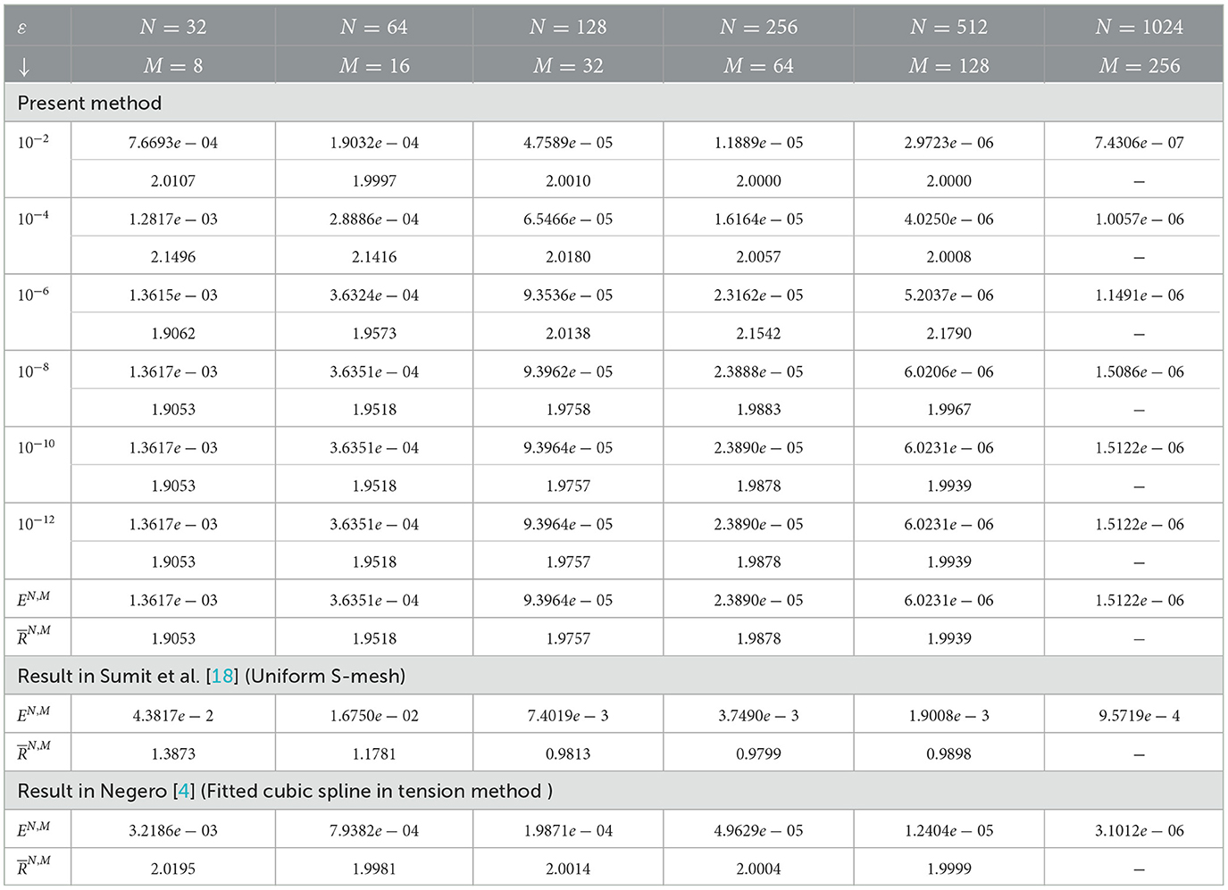
Table 1. Computed for example (5.1) at μ = 10−9 and comparison with Negero [4] and Sumit et al. [18].
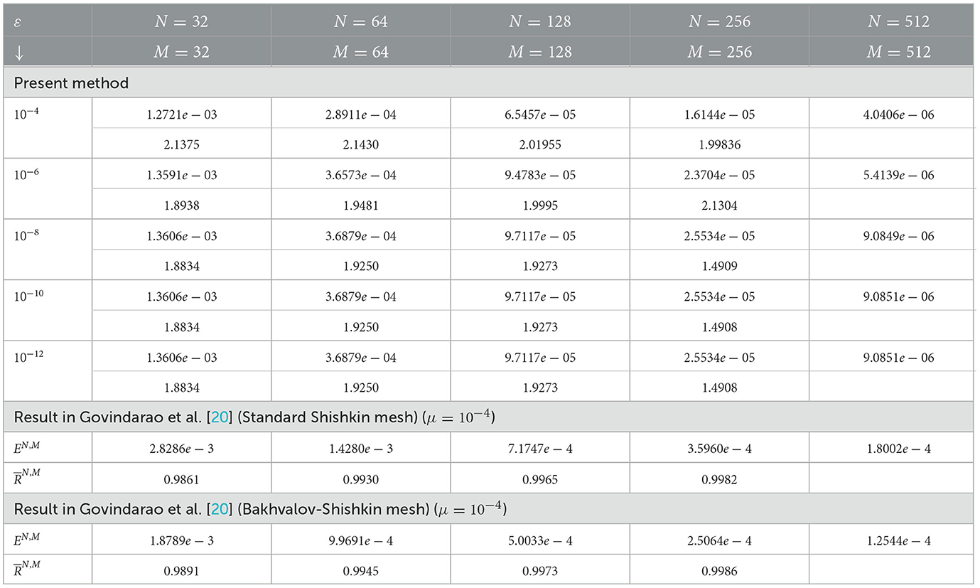
Table 2. Computed maximum point-wise error and rate of convergence for example (5.1) at μ = 10−4 and comparison with the study by Govindarao et al. [20] for N = M.
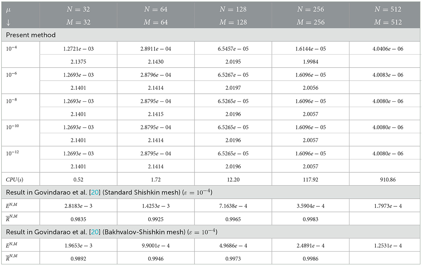
Table 3. Maximum point-wise error, convergence rate, and CPU time (in seconds) for example (5.1) with ε = 10−4 and N = M.
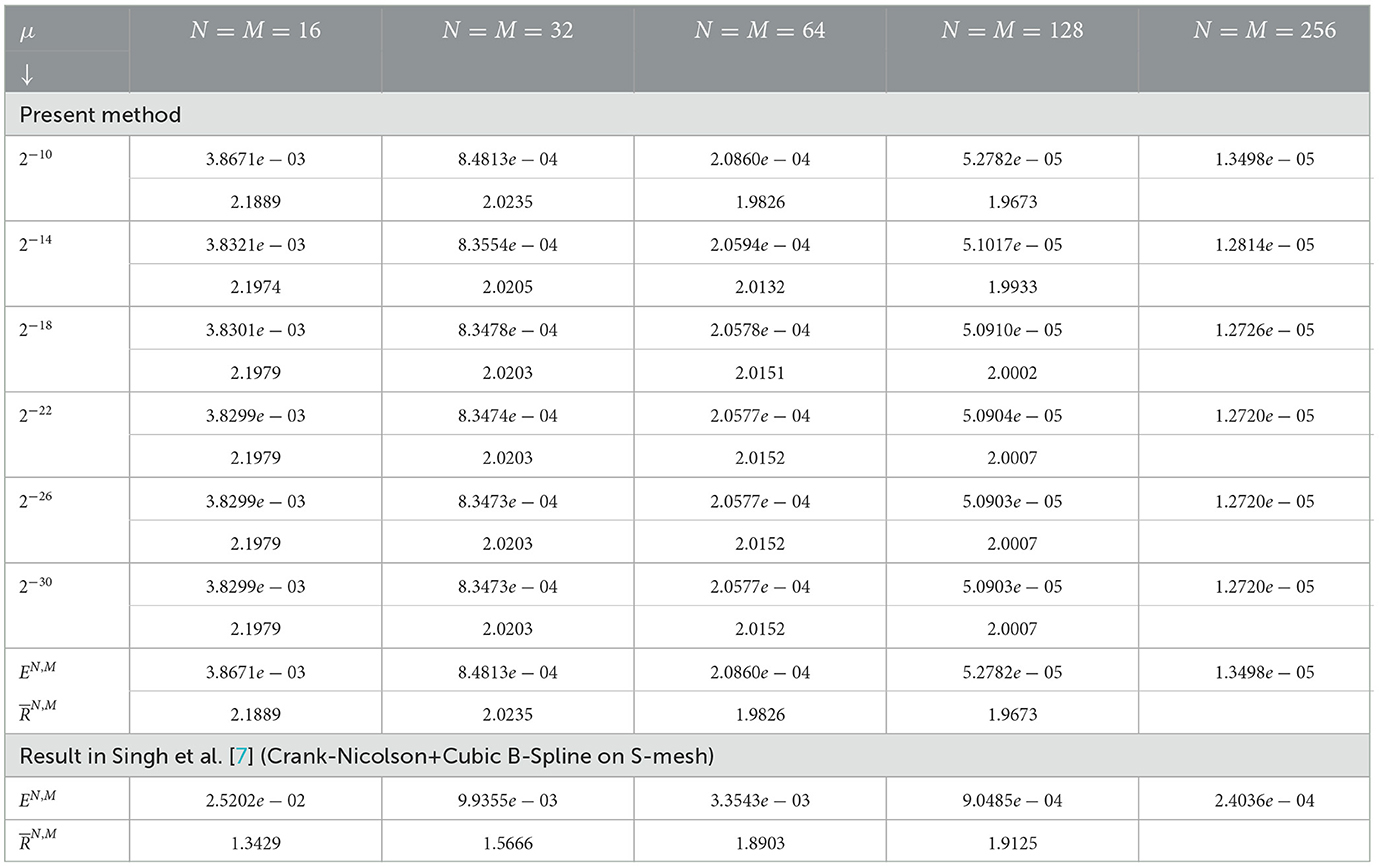
Table 4. Computed and for example (5.1) at ε = 2−10 and comparison with the study by Singh et al. [7] for varying values of μ.
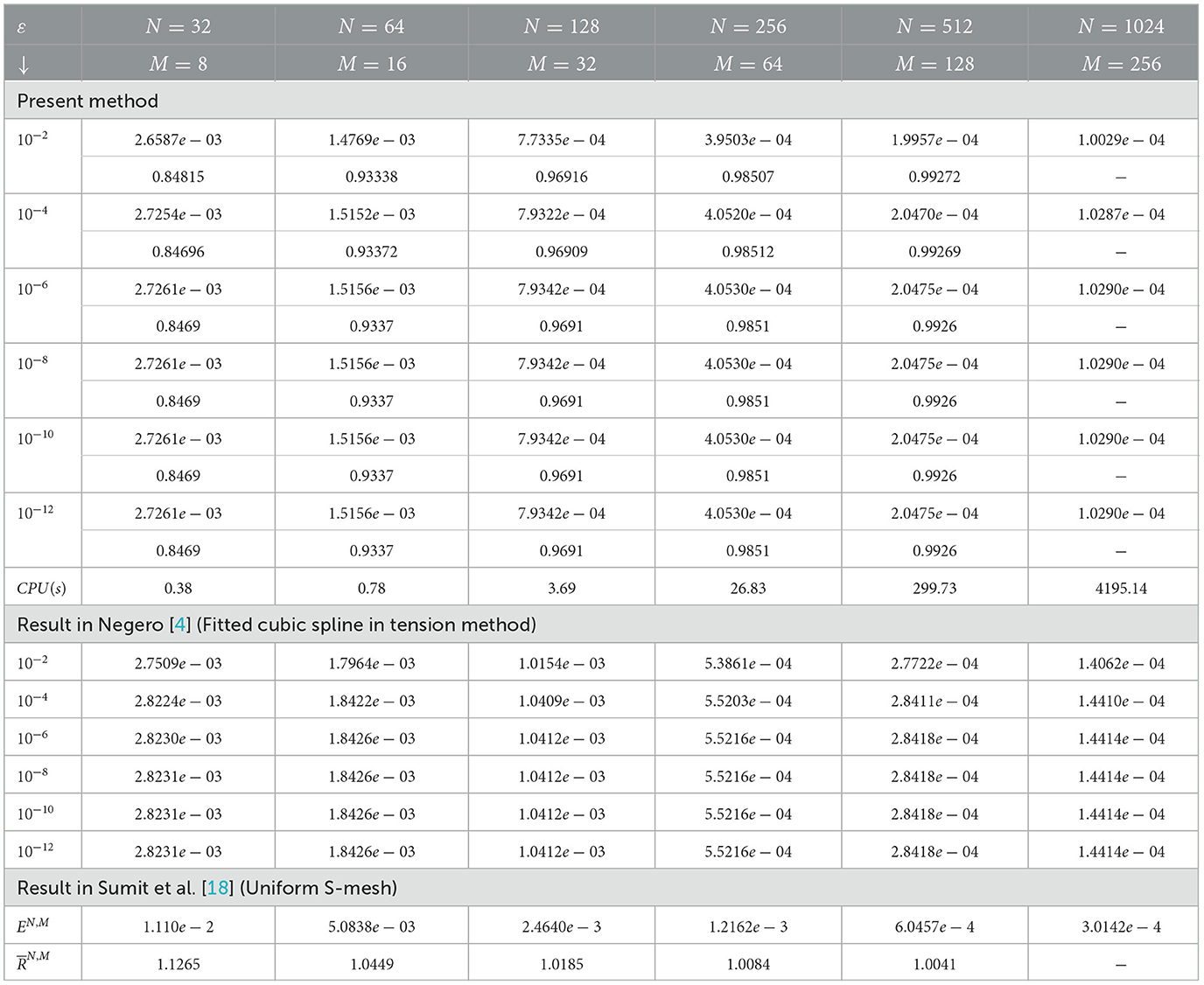
Table 5. Computed and CPU time (in seconds) for example (5.2) at μ = 10−9 and comparison with the study by Negero [4] and Sumit et al. [18].
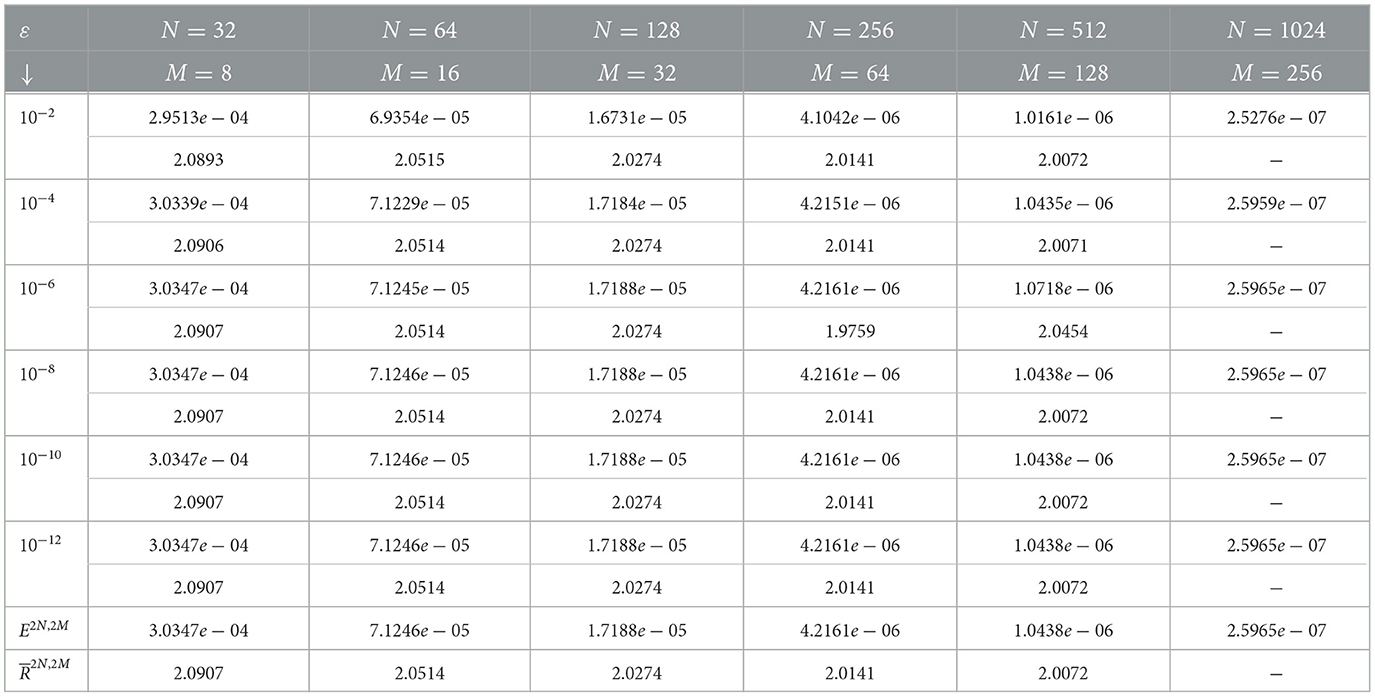
Table 6. Computed and for example (5.2) at μ = 10−9 after extrapolation.
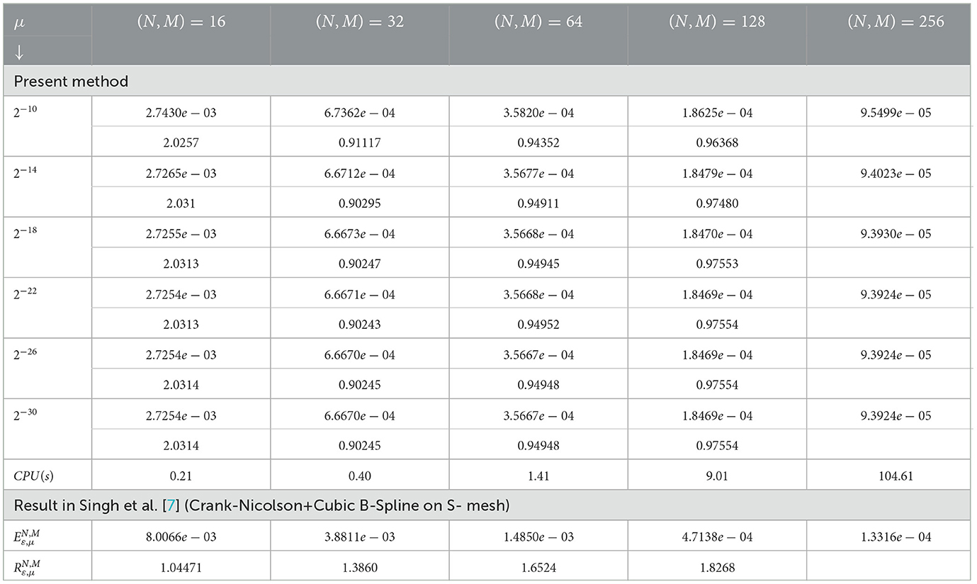
Table 7. Maximum point-wise error, convergence rate, and CPU time (in seconds) for example (5.3) with ε = 2−10 and varying μ values.

Table 8. Computed and for example (5.3) at ε = 10−10 after extrapolation.
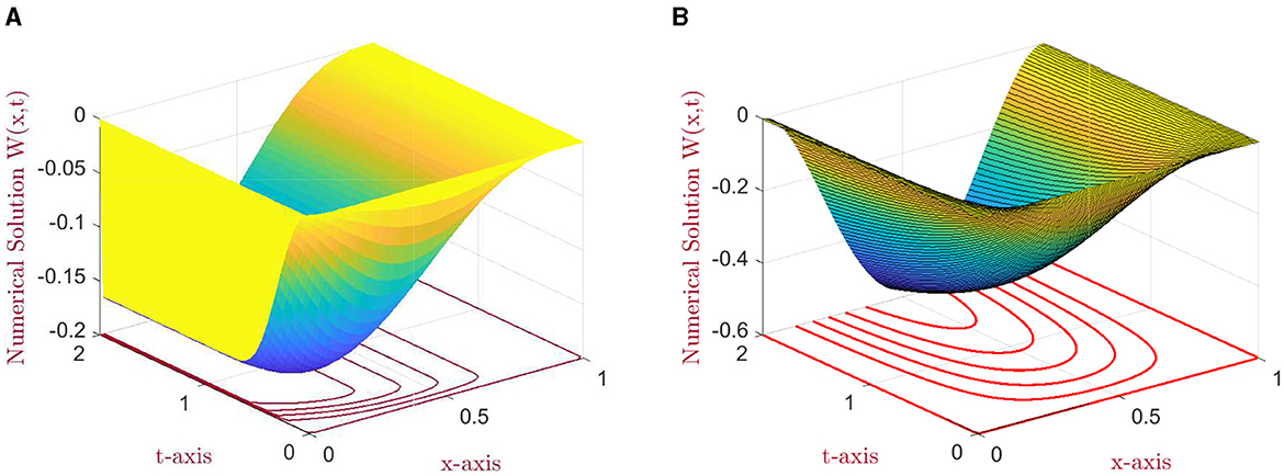
Figure 1. The numerical solution profile: (A) for N = M = 64, ε = 10−8, μ = 1, and (B) for N = M = 128, ε = 10−12, and μ = 10−10 for example (5.1).
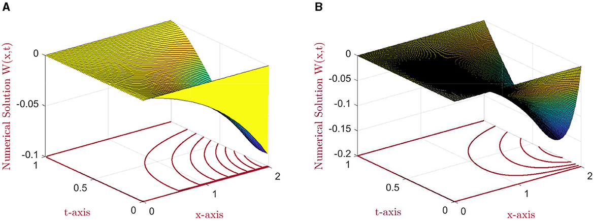
Figure 2. The numerical solution profile: (A) for N = M = 64, ε = 10−8, and μ = 1 and (B) for N = 256, M = 128, ε = 10−6, and μ = 10−10 for example (5.2).
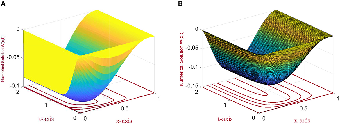
Figure 3. Surface plots of the numerical solutions: (A) for N = M = 64, ε = 2−18, and μ = 1 and (B) for N = M = 128, ε = 2−10, and μ = 2−10 for example (5.3).
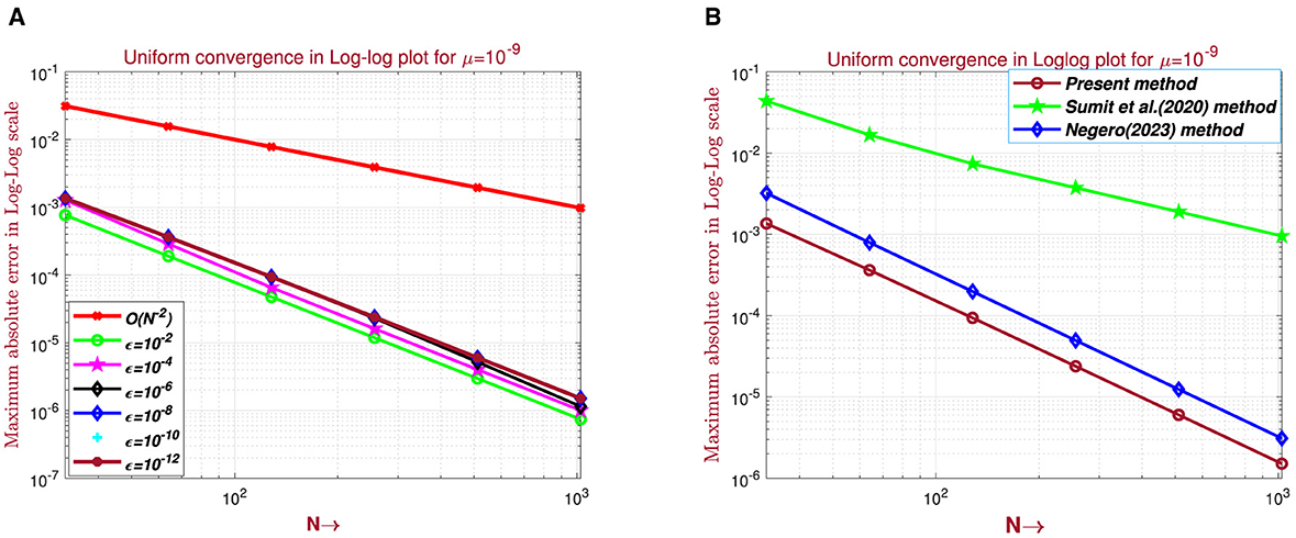
Figure 4. Log–log plot for example (5.1): (A) for Table 1 and (B) comparison of log–log plot with the existing literature.
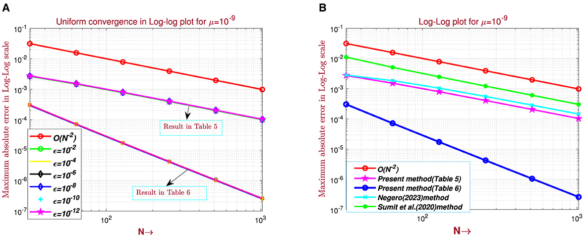
Figure 5. Log–log plot for example (5.2): (A) for Tables 5, 6 and (B) comparison of log–log plot with the existing literature.
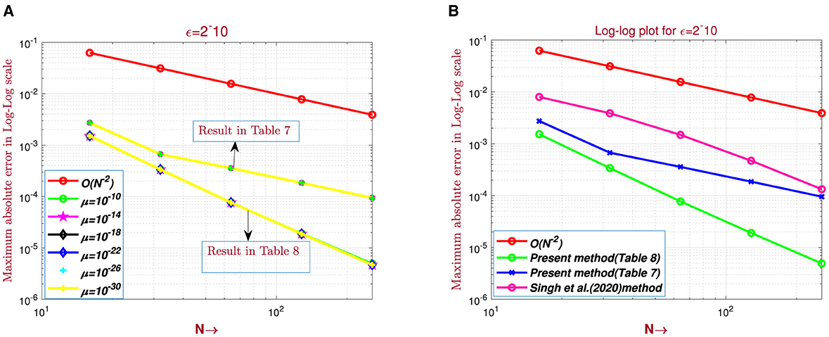
Figure 6. Log–log plot for example (5.3): (A) for Tables 7, 8 and (B) comparison of log–log plot with the existing literature.
For μ = 1, the considered problem belongs to the class of one-parameter time-delayed convection–diffusion parabolic problems, and a boundary layer of width O(ε) arises in the vicinity of x = 0, as shown in Figures 1A, 2A, 3A.
6 Conclusion
A two-parameter singularly perturbed time-delayed parabolic convection–diffusion problem is considered by the Crank–Nicolson method for the discretization of the time derivative, whereas in the discretization of the spatial variable, a numerical integration (1/3 rd Simpson's) formula is used by introducing an appropriate fitting factor. The method's novelty resides in its independence from delay terms, asymptotic expansions, and fitted meshes. The presence of two small parameters causes the problem to exhibit left and right boundary layers depending on the size of ε or μ. The method is demonstrated to have parameter uniform second-order convergence in both time and space. The performance of the proposed scheme is investigated by comparing the results, and it is discovered that the accuracy of the numerical results is comparable to or better than that of the existing difference schemes [4, 7, 18, 20], as verified both theoretically and numerically. To further demonstrate the versatility and applicability of the proposed approach, we highlight that the analysis method used in this study can be extended to high-order singularly perturbed time-delayed parabolic problems with Robin boundary conditions.
Data availability statement
The original contributions presented in the study are included in the article/supplementary material, further inquiries can be directed to the corresponding author.
Author contributions
SC: Conceptualization, Data curation, Formal analysis, Funding acquisition, Investigation, Methodology, Project administration, Resources, Software, Supervision, Validation, Visualization, Writing – original draft, Writing – review & editing. GD: Conceptualization, Investigation, Methodology, Validation, Writing – review & editing. TM: Conceptualization, Data curation, Formal analysis, Funding acquisition, Investigation, Methodology, Project administration, Resources, Software, Supervision, Validation, Visualization, Writing – original draft, Writing – review & editing.
Funding
The author(s) declare that no financial support was received for the research, authorship, and/or publication of this article.
Acknowledgments
The authors would like to thank the editor and reviewers for careful reading and giving prolific comments.
Conflict of interest
The authors declare that the research was conducted in the absence of any commercial or financial relationships that could be construed as a potential conflict of interest.
Publisher's note
All claims expressed in this article are solely those of the authors and do not necessarily represent those of their affiliated organizations, or those of the publisher, the editors and the reviewers. Any product that may be evaluated in this article, or claim that may be made by its manufacturer, is not guaranteed or endorsed by the publisher.
References
1. Kumar S, Kumar M. High order parameter-uniform discretization for singularly perturbed parabolic PDEs with time delay. Comput Math Appl. (2014) 68:1355–67. doi: 10.1016/j.camwa.2014.09.004
2. Clavero C, Jorge JC. An efficient and uniformly convergent scheme for one-dimensional parabolic singularly perturbed semilinear systems of reaction-diffusion type. Numer Algorithms. (2020) 85:1005–27. doi: 10.1007/s11075-019-00850-3
3. Wu J. Theory and Applications of Partial Functional Differential Equations, Vol. 119. Berlin: Springer Science & Business Media (2012).
4. Negero NT. Fitted cubic spline in tension difference scheme for two-parameter singularly perturbed delay parabolic partial differential equations. Partial Differ Equ Appl Math. (2023) 8:100530. doi: 10.1016/j.padiff.2023.100530
5. Schmitt J, DiPrima R. Asymptotic methods for an infinite slider bearing with a discontinuity in film slope. J Lubr Technol. (1976) 98:446–52. doi: 10.1115/1.3452885
6. Ayele MA, Tiruneh AA, Derese GA. Fitted cubic spline scheme for two-parameter singularly perturbed time-delay parabolic problems. Results Appl Math. (2023) 18:100361. doi: 10.1016/j.rinam.2023.100361
7. Singh S, Kumari P, Kumar D. An effective numerical approach for two parameter time-delayed singularly perturbed problems. Comput Appl Math. (2022) 41:337. doi: 10.1007/s40314-022-02046-3
8. Singh J, Kumar S, Kumar M. A domain decomposition method for solving singularly perturbed parabolic reaction-diffusion problems with time delay. Numer Methods Partial Differ Equ. (2018) 34:1849–66. doi: 10.1002/num.22256
9. Rao SCS, Kumar S. Second order global uniformly convergent numerical method for a coupled system of singularly perturbed initial value problems. Appl Math Comput. (2012) 219:3740–53. doi: 10.1016/j.amc.2012.09.075
10. Shivhare M, Podila PC, Kumar D. A uniformly convergent quadratic B-spline collocation method for singularly perturbed parabolic partial differential equations with two small parameters. J Math Chem. (2021) 59:186–215. doi: 10.1007/s10910-020-01190-7
11. Bhathawala P, Verma A. A two-parameter singular perturbation solution of one dimension flow through unsaturated porous media. Appl Math. (1975) 43:380–4.
12. DiPrima RC. Asymptotic methods for an infinitely long slider squeeze-film bearing. J Lubr Technol. (1968) 90:173–83. doi: 10.1115/1.3601534
13. Jazar RN. Perturbation Methods in Science and Engineering. Berlin: Springer (2021). doi: 10.1007/978-3-030-73462-6
14. Mekonnen TB, Duressa GF. Nonpolynomial spline method for singularly perturbed parabolic problem with two small parameters. Math Probl Eng. (2023) 2023:4798517. doi: 10.1155/2023/4798517
15. Hemker P, Shishkin G, Shishkina L. ε-uniform schemes with high-order time-accuracy for parabolic singular perturbation problems. IMA J Numer Anal. (2000) 20:99–121. doi: 10.1093/imanum/20.1.99
16. Shishkin GI. On finite difference fitted schemes for singularly perturbed boundary value problems with a parabolic boundary layer. J Math Anal Appl. (1997) 208:181–204. doi: 10.1006/jmaa.1997.5314
17. Duressa GF, Mekonnen TB. An exponentially fitted method for two parameter singularly perturbed parabolic boundary value problems. Commun Korean Math Soc. (2023) 38:299–318. doi: 10.4134/CKMS.c220020
18. Sumit, Kumar S, Kuldeep, Kumar M. A robust numerical method for a two-parameter singularly perturbed time delay parabolic problem. Comput Appli Math. (2020) 39:209. doi: 10.1007/s40314-020-01236-1
19. Priyadarshana S, Mohapatra J, Pattanaik S. Parameter uniform optimal order numerical approximations for time-delayed parabolic convection diffusion problems involving two small parameters. Comput Appl Math. (2022) 41:233. doi: 10.1007/s40314-022-01928-w
20. Govindarao L, Sahu SR, Mohapatra J. Uniformly convergent numerical method for singularly perturbed time delay parabolic problem with two small parameters. Iran J Sci Technol Trans A Sci. (2019) 43:2373–83. doi: 10.1007/s40995-019-00697-2
21. Gaspar F, Clavero C, Lisbona F. Some numerical experiments with multigrid methods on Shishkin meshes. J Comput Appl Math. (2002) 138:21–35. doi: 10.1016/S0377-0427(01)00365-X
22. Chen J, O'Malley R Jr. On the asymptotic solution of a two-parameter boundary value problem of chemical reactor theory. SIAM J Appl Math. (1974) 26:717–29. doi: 10.1137/0126064
23. Bigge J, Bohl E. Deformations of the bifurcation diagram due to discretization. Math Comput. (1985) 45:393–403. doi: 10.1090/S0025-5718-1985-0804931-X
24. O'Malley RE Jr. Two-Parameter Singular Perturbation Problems. Stanford, CA: Stanford University (1966).
25. O'malley R. Two-parameter singular perturbation problems for second-order equations. J Math Mech. (1967) 16:1143–1164.
26. Jha A, Kadalbajoo MK. A robust layer adapted difference method for singularly perturbed two-parameter parabolic problems. Int J Comput Math. (2015) 92:1204–21. doi: 10.1080/00207160.2014.928701
27. Das P, Mehrmann V. Numerical solution of singularly perturbed convection-diffusion-reaction problems with two small parameters. BIT Numer Math. (2016) 56:51–76. doi: 10.1007/s10543-015-0559-8
28. LinßT, Roos HG. Analysis of a finite-difference scheme for a singularly perturbed problem with two small parameters. J Math Anal Appl. (2004) 289:355–66. doi: 10.1016/j.jmaa.2003.08.017
30. Agbavon KM, Appadu AR, Khumalo M. On the numerical solution of Fisher's equation with coefficient of diffusion term much smaller than coefficient of reaction term. Adv Differ Equ. (2019) 2019:1–33. doi: 10.1186/s13662-019-2080-x
31. Appadu AR, Inan B, Tijani YO. Comparative study of some numerical methods for the Burgers-Huxley equation. Symmetry. (2019) 11:1333. doi: 10.3390/sym11111333
32. Agbavon KM, Appadu AR, Inan B, Tenkam HM. Convergence analysis and approximate optimal temporal step sizes for some finite difference methods discretising Fisher's equation. Front Appl Math Stat. (2022) 8:921170. doi: 10.3389/fams.2022.921170
33. Mohye MA, Munyakazi JB, Dinka TG. A nonstandard fitted operator finite difference method for two-parameter singularly perturbed time-delay parabolic problems. Front Appl Math Stat. (2023) 9:1222162. doi: 10.3389/fams.2023.1222162
34. Kehinde OO, Munyakazi JB, Appadu AR. A NSFD discretization of two-dimensional singularly perturbed semilinear convection-diffusion problems. Front Appl Math Stat. (2022) 8:861276. doi: 10.3389/fams.2022.861276
35. Alam MJ, Prasad HS, Ranjan R. An exponentially fitted integration scheme for a class of quasilinear singular perturbation problems. J Math Comput Sci. (2021) 11:3052–66. doi: 10.2891/jmcs/5589
36. Ranjan R, Prasad H. An efficient method of numerical integration for a class of singularly perturbed two point boundary value problems. WSEAS Trans Math. (2018) 17:265–73.
37. Reddy Y, Reddy KA. Numerical integration method for general singularly perturbed two point boundary value problems. Appl Math Comput. (2002) 133:351–73. doi: 10.1016/S0096-3003(01)00246-6
38. Clavero C, Jorge J, Lisbona F. A uniformly convergent scheme for convection-diffusion parabolic problems. J Comput Appl Math. (2003) 154:415–29. doi: 10.1016/S0377-0427(02)00861-0
39. Doolan EP, Miller JJ, Schilders WH. Uniform Numerical Methods for Problems with Initial and Boundary Layers. Dublin: Boole Press (1980).
Keywords: singularly perturbed problems, delay parabolic differential equation, numerical integration, Simpson's 1/3rd rule, parameter-uniform
Citation: Cheru SL, Duressa GF and Mekonnen TB (2024) Numerical integration method for two-parameter singularly perturbed time delay parabolic problem. Front. Appl. Math. Stat. 10:1414899. doi: 10.3389/fams.2024.1414899
Received: 09 April 2024; Accepted: 28 June 2024;
Published: 15 July 2024.
Edited by:
Eun-Jae Park, Yonsei University, Republic of KoreaReviewed by:
Sunil Kumar, Indian Institute of Technology (BHU), IndiaAppanah Rao Appadu, Nelson Mandela University, South Africa
Copyright © 2024 Cheru, Duressa and Mekonnen. This is an open-access article distributed under the terms of the Creative Commons Attribution License (CC BY). The use, distribution or reproduction in other forums is permitted, provided the original author(s) and the copyright owner(s) are credited and that the original publication in this journal is cited, in accordance with accepted academic practice. No use, distribution or reproduction is permitted which does not comply with these terms.
*Correspondence: Tariku Birabasa Mekonnen, c2VlbmFhMjlAZ21haWwuY29t