
95% of researchers rate our articles as excellent or good
Learn more about the work of our research integrity team to safeguard the quality of each article we publish.
Find out more
ORIGINAL RESEARCH article
Front. Appl. Math. Stat. , 26 July 2024
Sec. Mathematical Physics
Volume 10 - 2024 | https://doi.org/10.3389/fams.2024.1412181
 Ratesh Kumar
 Sonia Arora*
A novel Haar scale-3 wavelet collocation technique is proposed in this study for dealing with a specific type of parabolic Buckmaster second-order non-linear partial differential equation in a dispersive system and Chafee–Infante second-order non-linear partial differential equation (PDE) in a solitary system. Using Haar scale-3 (HSW-3) wavelets, the system approximates the space and time derivatives. To develop both an implicit and explicit analytical model for the dispersive and solitary system, the collocation approach is employed in conjunction with the discretization of space and time variables. We have examined the effectiveness, applicability, and veracity of the proposed computational approach using a variety of numerical problems with nonlinearity and numerous significant source terms. Additionally, the outcomes are graphically presented and organized. We achieved accuracy with the proposed methods even with a small selection of collocation locations.
Physical, chemical, and natural science fields all often use the non-linear PDE governing equations. These equations have been the subject of extremely quick research. Researchers often struggle to come up with analytical answers to non-linear situations. Therefore, a numerical solution comes to the rescue when an analytical solution to the problem cannot be found. Initially used as a potent tool in data compression and signal and picture processing, wavelet theory is currently used in many other fields. One of the simplest wavelets, the Haar wavelet, enables sparse representation since the wavelet expansion of a function has many small coefficients. The Haar wavelet basis has several advantages for its use in applied mathematics. For instance, it can efficiently relocate in both time and space, has local structural features, and provides compactly supported orthonormal wavelets. As a result, these properties make the Haar wavelet basis an attractive choice for mathematicians who need to use wavelets for numerical computations.
The basic goal of numerical algorithms is to reduce error while requiring fewer resources. To meet these conditions for solving this form of partial differential equation, the Haar wavelet is a promising tool since it can track the singularity and boost the local grid resolution by introducing higher resolutions. Lower resolutions can be used to calculate the findings in smoother regions.
Two PDEs with non-linear components are examined in this study since they are renowned for having a wide range of potential implementations.
i. Buckmaster second-order partial differential equation
ii. Chafee–Infante second-order partial differential equation
A parabolic non-linear partial differential equation with two non-linear terms is the Buckmaster equation. This equation is used to describe large-scale and long-term deformation and is regarded as a model of a dispersive system. The Haar Scale-3 well-defined wavelet collocation method has been used to numerically solve the Buckmaster non-linear partial differential equation. Two non-linear terms make up the non-linear partial differential equation which is known as the Buckmaster equation. The dispersive model is implemented using this equation.
The generic equation for the Buckmaster equation is provided by
under the following initial constraints
The applied boundary condition is as follows:
where is a well-known constant which is known as the wavelength of the wave. , , , and are the provided functions clearly defined and specified, and is the function for which the value is sought.
The general Chafee–Infante (GCI) non-linear partial differential equation is taken into consideration to demonstrate the originality and benefits of this approach, and numerous new precise wave solutions are produced uniformly. One non-linear term makes up the non-linear partial differential equation known as the Chafee–Infante equation. The solitary wave model is implemented using this equation.
under the following initial constraints
The applied boundary condition is as follows:
where is a well-known constant which is known as phase velocity periodic function. , , , and are the well-defined functions, and is the function that needs to be determined.
Many mathematical models of geological, economic, and natural evolution are based on partial differential equations, and more recently, their application has expanded to include domains such as accounting, investment analysis, and image recognition (1). Since these types of problems frequently have numerical or approximative solutions available (2–8), it is practically difficult to solve most non-linear and certain linear differential equations using exact solutions. The non-linear nature of the differential equation makes it difficult to answer analytically, and its high-order derivatives correlate to both time and space. Finding the answer to these equations becomes a challenging job because there is no proven empirical strategy for resolving this kind of problem. As a result, many investigators are working to develop novel computational and semi-analytical methods for determining solutions to the diverse issues controlled by Buckmaster equations. Among the recently created and used techniques for solving, the Buckmaster equations are the Adams–Bashforth method (ABM) (9), Finite Volume Method (FVM) (10), B-Spline collocation method (BSCM) (11), and Method of lines (MOL) (12). For the Chafee–Infante equation, many investigations are exponential method (EXP) (13), canonical-like transformation method (CTM) (14), and Laplacian Operator Method (LOM) (15). The examples are compared with the precise solutions to demonstrate the accuracy, convergence, and effectiveness of the proposed method and highlight the excellent approximate solutions that are obtained. Additionally, other literature references are used to support these claims.
The wavelet approach has been widely employed in image digital processing, general relativity, mathematical methods, and many other domains in recent years as a powerful mathematical weapon. The formulae for the father wavelet (FW) and mother wavelet (MW) in the Scale 3 wavelet family with dilation factor 3 are presented in equations 3–5.
A non-linear system of partial differential equations of second and fifth orders is solved using the Scale-3 Haar wavelet integral approach. Any square adaptable integrable function specified in the range [0, 1] can be written exclusively in terms of the infinite sum of the Haar pattern attributable to the orthogonality condition in wavelets (16–18).
Haar Scaling Function
By applying this relationship to different dilations and translations of , a wavelet family consisting of and so on can be obtained. Among these wavelets, and are referred to as mother wavelets, while the remaining wavelets are referred to as daughter wavelets.
Let us define the collocation points and discredit the Haar function ; in this way, we get the coefficient matrix which has the dimension 3 M*3 M. The 3 M square matrix that serves as the operational matrix for the integration of P is defined. A differential equation of any order is being solved. Specifically, we use the integral method to integrate the Haar Scale-3 wavelets (19, 20).
Moreover, we introduce
The method of quasi-linearization finds application in the solution of two-point and multi-point boundary value problems for linear and non-linear ordinary differential equations, boundary value problems for elliptic and parabolic partial differential equations, variational problems, differential-difference, and functional-differential equations. As with every iteration scheme, the method of quasi-linearization is suitable for computer implementation and has various modifications enabling one to accelerate the convergence for narrower classes of problems (16, 17). The quasi-linearization approach is an extended version of the Newton–Raphson method used to linearize non-linear differential equations. It exhibits quadratic convergence toward the exact solution, assuming convergence exists, and the convergence is monotonic. This technique is employed because there is often no analytical method available to solve numerous non-linear equations, and societal demands necessitate finding solutions for these equations. Equations (1) and (2) are a non-linear term, and we have to use the below recurrence relation (21–29):
where is a non-linear function of and , and each step will have a known value that will be utilized to calculate .
To linearize the non-linear term in equations (1) and (2), the quasi-linearization technique described above can be applied.
For the First Non-linear term:
For the Second Non-linear term:
The third Non-linear term:
After applying the quasi-linearization, we have equations (13) and (14) then using these, non-linear systems of the partial differential equation (1) transformed into the series of the linear differential equation (16) we have
under the following variety of initial constraints
The boundary condition
Here, represents approximation for t (time) in the process of quasi-linearization
When the aforementioned statement is used to integrate the equation (17), which has a domain from 0 to r, it results in
The result is obtained by integrating and defining the equation (18), concerning r, within the defined domain from 0 to 1.
Equation (18) is obtained by substituting the value of from equation (19)
Once more, by integrating the expression and defining it concerning s within the bounds of s, we have
Once more, choosing limits 0 to t and integrating about t, we have
Differentiating equation (22) concerning r we get
Differentiating equation (23) concerning r we get
Put all the values from equations (17)–(24) in (16) then given PDE becomes from equations (12)– (25)
The abovementioned expression is reduced to an algebraic equation system, which is further reduced to the defined system of 4D arrays below.
Additionally, the aforementioned array system can be simplified and represented as a well-defined system in matrix form.
Subsequently, by employing the Thomas technique in a MATLAB application, the values of the matrix can be sequentially determined for various defined values of n (ranging from 1 to 3 and so on). This matrix structure described above can then be utilized to recover the original wavelet coefficient .
After applying the quasi-linearization, we have equation (15), and then using this, non-linear system of the partial differential equation (2) transformed into the series of the linear differential equations (26) we have:
under the following variety of initial constraints:
The boundary condition
Here, represent approximation for t in the process of quasi-linearization.
When the abovementioned statement is used to integrate the equation (27), which has a domain from 0 to s, it results in
The result is obtained by integrating and defining the equation (18), concerning s, within the defined domain from 0 to 1.
Equation (18) is obtained by substituting the value of from equation (19)
Once more, by integrating the expression and defining it about s within the bounds of s, we have
Now, furthermore, integrating concerning s and taking limits 0 to s we have:
Differentiating (22) concerning r we get:
Differentiating (23) concerning x we get:
Put all the values from equations (27)–(34) in (26) then the equation becomes:
The abovementioned expression is reduced to an algebraic equation system, which is further reduced to the defined system of 4D arrays below.
Furthermore, the above array system can be diminished to the well-defined matrix form system.
The matrix values can be determined sequentially for various predefined values of n (such as 1, 2, and 3) using the Thomas technique within a MATLAB application. This approach allows for the solution of the system of equations. Moreover, the matrix structure mentioned earlier can be employed to recover the original wavelet coefficient .
If is any differentiable function such that for all t for some positive real constant M and is approximated by the Haar wavelet family as given below:
Then, the error bound was calculated for the Haar wavelet approximation of the function by -norm is given as follows:
If the exact value of M is known, it is possible to obtain the precise error bound for the approximation equations (38, 39). Furthermore, as the level of resolution increases (the value of , the error decreases, providing evidence of convergence between the approximate solutions and the exact solution. This notion of convergence is also demonstrated through numerical experiments conducted below.
MATLAB is a proprietary multi-paradigm programming language, and numeric computing environment developed by MathWorks MATLAB allows matrix manipulations, plotting of functions and data, implementation of algorithms, creation of user interfaces, and interfacing with programs written in other languages. Although MATLAB is intended primarily for numeric computing, an optional toolbox allows access to symbolic computing abilities. The computer program MATLAB was utilized for numerical computations and generating graphical results. To compute the solution of a second-order non-linear partial differential equation (PDE) using the Haar measure-3 wavelet, it is crucial to have a discrete and well-defined representation of the Haar measure-3 wavelet pattern. To achieve this, collocation points are selected at the previously mentioned point of discontinuity in the provided equations. Specifically, for the Haar Scale-3 wavelet matrix, the collocation points are chosen at the first level of resolution, corresponding to j = 1. The effectiveness of the proposed scheme was evaluated by solving three problems using the described approach and computing the absolute defined errors. This evaluation aimed to demonstrate the suitability of the current scheme for solving the Buckmaster equation.
1. Input: Lower and Upper limit of Haar function including the level of resolution.
2. Step-1: Assume the space approximation from equations (17) and (28).
3. Step-2: Assume the time approximation from the same combined equations (17) and (28).
4. Step-3: Apply the Haar Scale-3 integrals from equations (17) to (27) to and (28) to (37).
5. Step-4: Then, substitute all the derivatives and integrals in given equations and solve the matrix form of linear equation with different levels of resolution.
6. Output: Errors and graphical representation for different levels of resolution.
We are going to consider the following type of specified non-linear Buckmaster equation in the required form as follows:
Subjected to the well-defined boundary condition
The defined initial condition that has been provided is the form
With source term
From our previous literature for the abovementioned problem, the exact solution is:
Using the current approximation approach for λ = 1, we proposed the numerical solution below with the help of equations (40) to (44).
The graphical presentation of example-1 in Figure 1 depicts the approximate and the exact answers with the absolute error. The compatibility of the exact and estimated answers for J = 1 is shown in Figure 1. The data given above in tabular form demonstrate that solutions are reliable and complementary over a range of values of J = 1, 2, and 3. The outcomes for errors for J = 1, 2, and 3 are shown in Table 1.
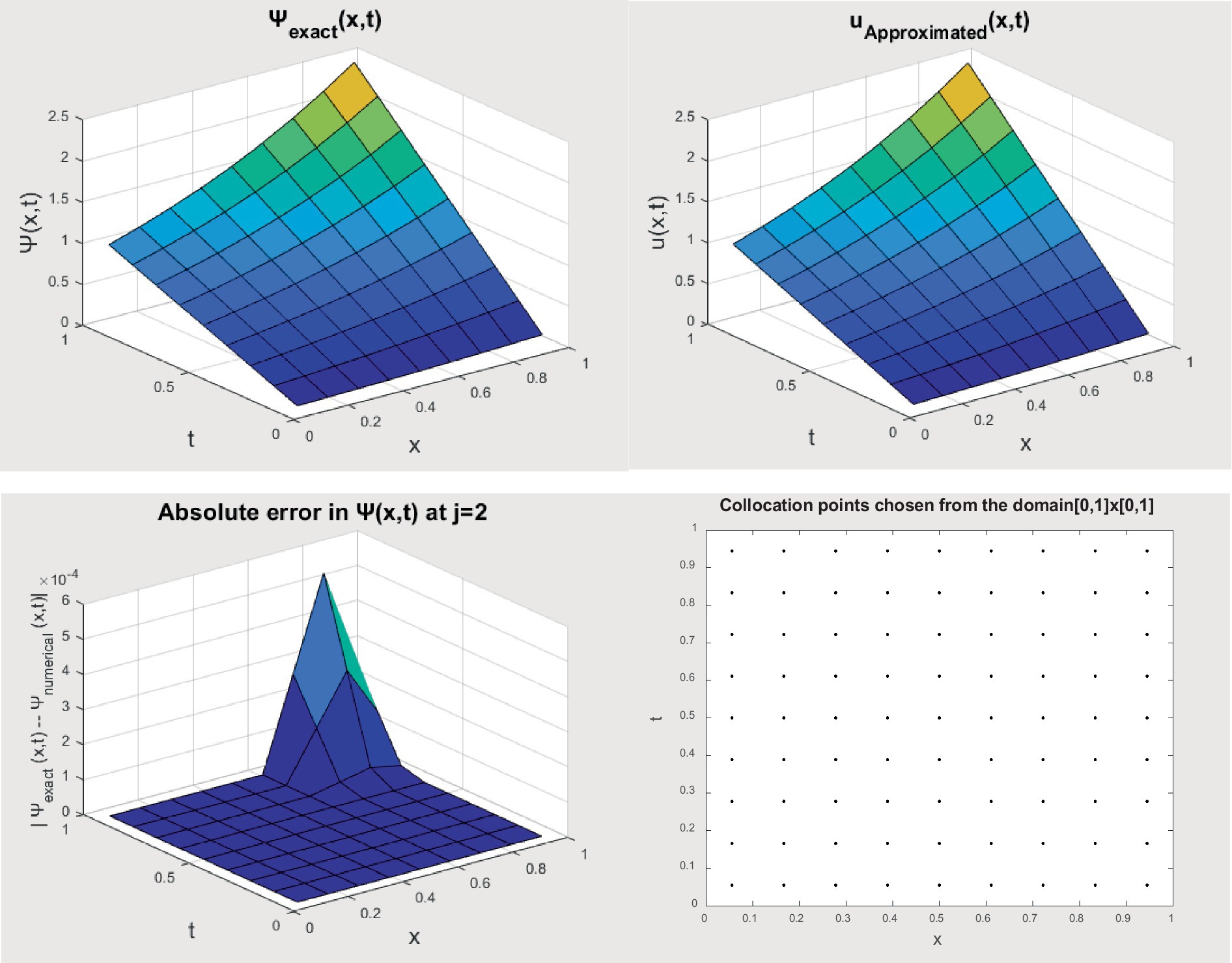
Figure 1. Graphical representation for the abovementioned numerical problem-1.
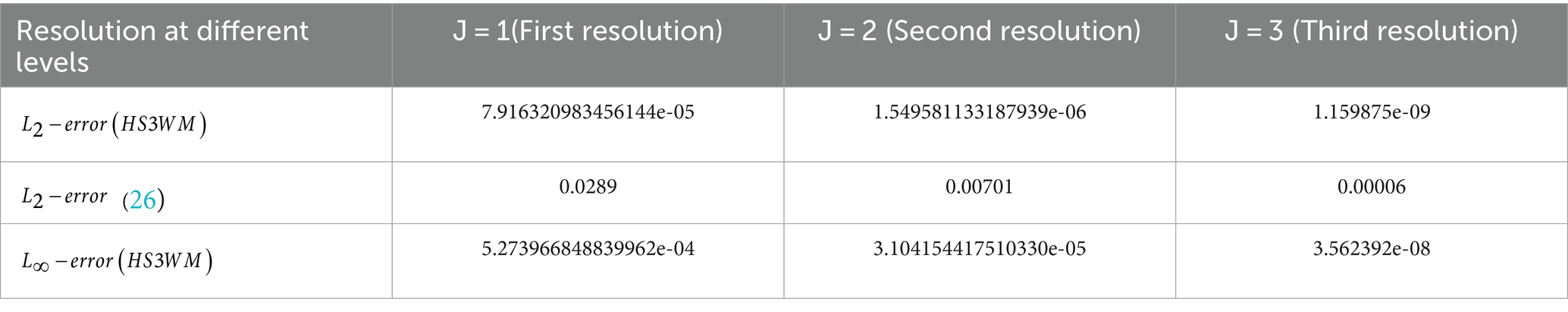
Table 1. errors at many different values of J for the abovementioned numerical problem – 1.
We will assume the following specified non-linear Buckmaster equation in the required form of
in the presence of the boundary condition
In addition, the defined initial condition that has been provided and has the form
With source term
The precise solution to this problem is found in our literature and is
Using the current approximation approach for λ = 1, we proposed the numerical solution below with the help of equations (45) to (49).
The graphical presentation of example-2 in Figure 2 depicts the approximate and the exact answers with the absolute error. The compatibility of the exact and estimated answers for J = 1 is shown in Figure 2. The data given above in tabular form demonstrate that solutions are reliable and complementary over a range of values of J = 1, 2, and 3. The outcomes for errors for J = 1, 2, and 3 are shown in Table 2.
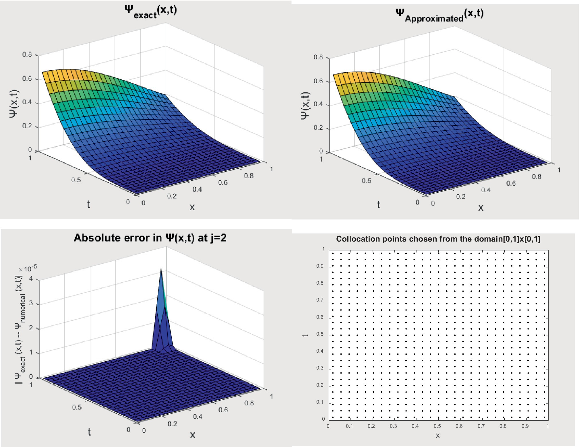
Figure 2. Graphical representation for the abovementioned numerical problem-2.
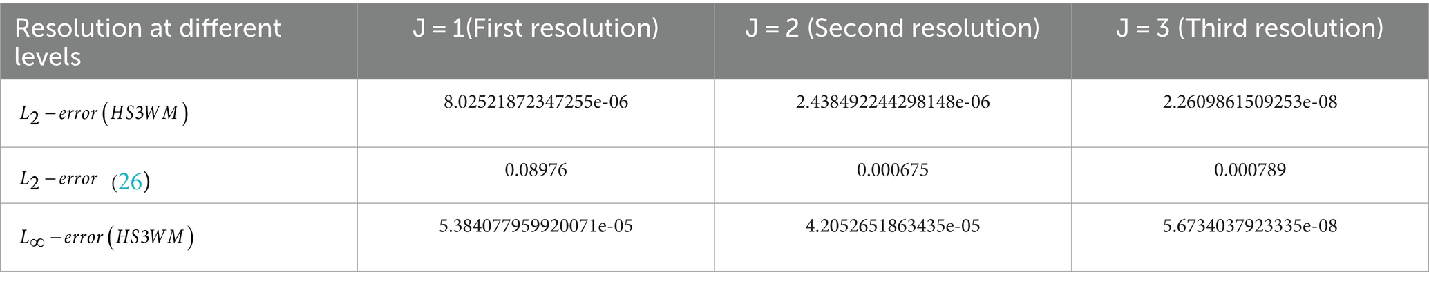
Table 2. errors at many different values of J for the abovementioned numerical problem – 2.
In the well-defined third numerical problem, we are going to consider in this way the non-linear Chaffee–Infante equation in the required form which is
Subjected to the well-defined boundary condition
Moreover, the initial condition which is of the form
With source term
The precise solution to this problem is found in our literature and is
Using the current approximation approach for λ = 1, we proposed the numerical solution below with the help of equations (50) to (54).
The graphical presentation of example-3 in Figure 3 depicts the approximate and the exact answers with the absolute error. The compatibility of the exact and estimated answers for J = 1 is shown in Figure 3. The data given above in tabular form demonstrate that solutions are reliable and complementary over a range of values of J = 1, 2, and 3. The outcomes for errors for J = 1, 2, and 3 are shown in Table 3, and it can be concluded that the errors are reduced by increasing the level of resolution which ensures the convergence of the method. In addition, we have used an adaptive grid to find CPU time, which is for all three examples is the same.
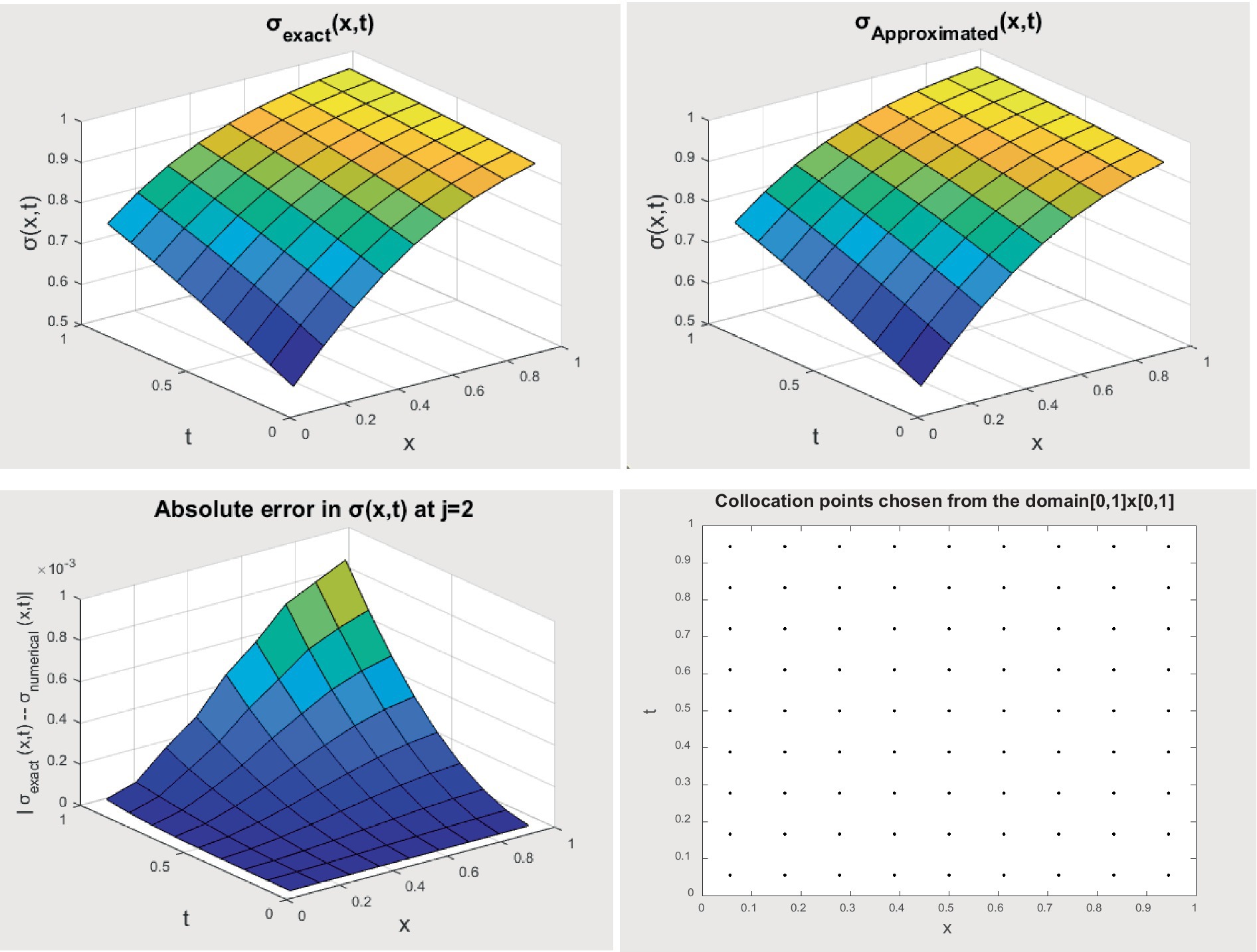
Figure 3. Graphical representation for the abovementioned numerical problem-3.
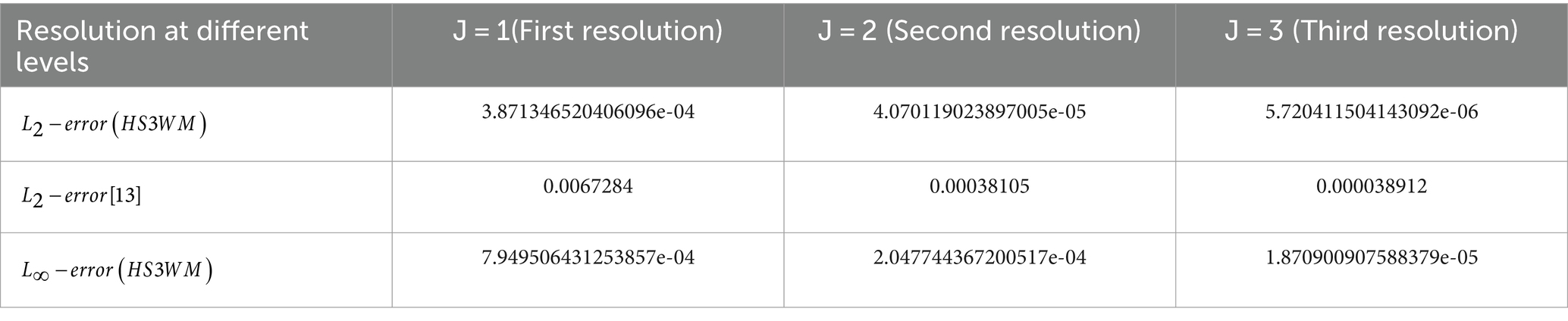
Table 3. errors at many different values of J for the abovementioned numerical problem – 3.
In this study, a hybrid wavelet methodology for the Haar Scale-3 is proposed as a discretization. To demonstrate the effectiveness of the approach, it has been used for the non-linear Buckmaster equation and Chaffee–Infante equation problems. The following benefits of the suggested plan:
1. The numerical studies showed that efficiency is reached with greater time step sizes than those employed by previous approaches. This signifies that the proposed approach requires x (or t) to be quite small.
2. To handle non-linear factors, the suggested numerical method does not need any filtering methods. To transform non-linear terms into linear terms, we used the quasi-linearization method.
3. The suggested methodology is reliable, straightforward, and efficient. Even though there are a limited number of collocation locations, accuracy is still strong.
4. The method is easy to use on computers and incurs low computing costs.
When compared to other methods and exact solutions, the method is effective and accurate for a variety of non-linear equations.
The raw data supporting the conclusions of this article will be made available by the authors, without undue reservation.
RK: Conceptualization, Data curation, Formal analysis, Funding acquisition, Investigation, Methodology, Project administration, Resources, Software, Supervision, Validation, Visualization, Writing – original draft, Writing – review & editing. SA: Conceptualization, Data curation, Formal analysis, Funding acquisition, Investigation, Methodology, Project administration, Resources, Software, Supervision, Validation, Visualization, Writing – original draft, Writing – review & editing.
The author(s) declare that no financial support was received for the research, authorship, and/or publication of this article.
The authors declare that the research was conducted in the absence of any commercial or financial relationships that could be construed as a potential conflict of interest.
All claims expressed in this article are solely those of the authors and do not necessarily represent those of their affiliated organizations, or those of the publisher, the editors and the reviewers. Any product that may be evaluated in this article, or claim that may be made by its manufacturer, is not guaranteed or endorsed by the publisher.
1. Al-Aimri, A., Numerical treatment for solving Systems of Nonlinear Differential Equations, m.Sc. Thesis, University of Al-Mustansiriyah, (2009).
2. Coudiére, Y., Gallouët, T., and Herbin, R., Discrete Sobolev inequalities and L2 error estimates for approximate finite volume solution of convection-diffusion equation. Modélisation mathématique et analyse numérique, (2001) 35:767–778.
3. Christie, I, Griffiths, D, Mitchell, A, and Zienkiewicz, O. Finite element methods for second order differential equations with significant first derivatives, international numerical mathematical. Engineering. (1976) 10:1389–96. doi: 10.1002/nme.1620100617
4. Caldwell, J, and Wanless,. Finite element approach to Burger’s equation. App Math Modeling. (1981) 5:189–93. doi: 10.1016/0307-904X(81)90043-3
5. Donea, J, Giuliani, S, and Laval, H. Finite element solution of the unsteady Navier-stokes equation by fractional step method, app. Mech Eng. (1982) 30:53–73. doi: 10.1016/0045-7825(82)90054-8
6. Garrouch, AA, and Al-Dousari, MM. Applying the finite volume method for solving the convection- dispersion equation in radial coordinates. Int J of Petroleum Sci and Tech. (2007) 1:75–97.
7. Moshiour, R. Finite volume methods for solving hyperbolic pdes on curved manifolds. BRAC J Uni. (2005) II:99–103.
8. Kadhum, Shaimaa Abdul-Hussain, The maximum principle and error estimate of the upwind finite volume method for nonlinear convection-diffusion equation, m.Sc. Thesis, University of Basrah, (2010)
9. Haq, Ihtisham Ul, Ali, Nigar, Ahmad, Shabir, and Akram, Tayyaba, A hybrid interpolation method for fractional PDEs and its applications to fractional diffusion and Buckmaster equations, mathematical problems in engineering. App. Mech. Eng. (2013). 30, 77–93.
10. Goh, J., B-splines for initial and boundary value problems, Ph.D. thesis, University Sains Malaysia. (2012).
11. Evans, G, Blackledge, J, and Yardley, P. Numerical methods for partial differential equations. London: Springer Verlag (2001).
12. Ames, W. Numerical methods for partial differential equation. New York, San Francisco: Academic Press (1977).
13. Sakthivel, Rathinasamy, and Chun, Changbum, New soliton solutions of Chaffee-Infante equations using the Exp-function method, Zeitschrift fur Naturforschung (2022).
14. Mao, Yuanyuan, Exact solutions to (2 + 1)-dimensional Chaffee–Infante equation, Pramana journal physics (2018)
15. Huang, H, and Huang, R. Sign changing periodic solutions for the Chafee–Infante equation. Appl Anal. (2017) 97:2313–31. doi: 10.1080/00036811.2017.1359570
16. Ratesh, K. Investigation for the numerical solution of Klein-Gordon equations using scale-3 Haar wavelets. J Phys Conf Ser. (2022) 2267:012152. doi: 10.1088/1742-6596/2267/1/012152
17. Ratesh, Kumar, Haar (scale 3) wavelet-based solution of 1D-hyperbolic telegraph equation think. India Journal. (2019)
18. Ratesh, Kumar, New scheme for the solution of (2+1)-dimensional non-linear partial differential equations using 2D-Haar scale 3 wavelets and −weighted differencing. Journal of EmergingTechnologies and Innovative Research. (2019).
19. Ratesh, Kumar, A hybrid scheme based upon non-dyadic wavelets for the solution of linear Sobolev equations. differencing. Journal of EmergingTechnologies and Innovative Research. (2019).
20. Ratesh, Kumar, Historical development in Haar wavelets and their application - an overview. differencing. Journal of EmergingTechnologies and Innovative Research. (2018).
21. Delkhosh, M, and Parand, K. A hybrid numerical method to solve nonlinear parabolic partial differential equations of time-arbitrary order. Comput Appl Math. (2019) 38. doi: 10.1007/s40314-019-0840-6
22. Lin, B. A new numerical scheme for third-order singularly Emden-fowler equations using quintic B-spline function. Int J Comput Math. (2021) 98:2406–22. doi: 10.1080/00207160.2021.1900566
23. Arafa, A, Khaled, O, and Hagag, A. Analytical and approximate solutions for fractional Chaffee–Infante equation. Int J Appl Comput Math. (2023) 9:47–88. doi: 10.1007/s40819-023-01514-6
24. Izadi, M, and Zeidan, D. A convergent hybrid numerical scheme for a class of nonlinear diffusion equations. Comput Appl Math. (2022) 41. doi: 10.1007/s40314-022-02033-8
25. Tahir, M, Sunil, KD, Rehman, H, Ramzan, M, Hasan, A, and Osman, M. Exact traveling wave solutions of Chaffee-Infante equation in (2+1)-dimensions and dimensionless Zakharov equation. Mathematical Methods in the Applied Sci. (2021) 44:1500–13. doi: 10.1002/mma.6847
26. Ramos, H, Kaur, A, and Kanwar, V. Using a cubic B-spline method in conjunction with a one-step optimized hybrid block approach to solve nonlinear partial differential equations. Comput Appl Math. (2022) 41:89–115. doi: 10.1007/s40314-021-01729-7
27. Sinha, AK. Introducing higher-order Haar wavelet method for solving three-dimensional partial differential equations. Int J Wavelets Multiresolution Inf Process. (2024) 22:2350040
28. Asif, Muhammad, Bilal, Faisal, and Khan, Imran. (2024). Extension of Haar wavelet technique for numerical solution of three-dimensional linear and nonlinear telegraph equations. Partial Differential Equations in Applied Mathematics. 575–597.
Keywords: quasilinearization technique, Buckmaster, collocation points, dispersive system, solitary system
Citation: Kumar R and Arora S (2024) Application of Haar Scale-3 wavelet method to the solution of Buckmaster and Chaffee–Infante non-linear PDE. Front. Appl. Math. Stat. 10:1412181. doi: 10.3389/fams.2024.1412181
Edited by:
Yusuf Gurefe, Mersin University, TürkiyeReviewed by:
Youssri Hassan Youssri, Cairo University, EgyptCopyright © 2024 Kumar and Arora. This is an open-access article distributed under the terms of the Creative Commons Attribution License (CC BY). The use, distribution or reproduction in other forums is permitted, provided the original author(s) and the copyright owner(s) are credited and that the original publication in this journal is cited, in accordance with accepted academic practice. No use, distribution or reproduction is permitted which does not comply with these terms.
*Correspondence: Sonia Arora, c29uaWFkZWxoaXRlQGdtYWlsLmNvbQ==
Disclaimer: All claims expressed in this article are solely those of the authors and do not necessarily represent those of their affiliated organizations, or those of the publisher, the editors and the reviewers. Any product that may be evaluated in this article or claim that may be made by its manufacturer is not guaranteed or endorsed by the publisher.
Research integrity at Frontiers
Learn more about the work of our research integrity team to safeguard the quality of each article we publish.