 Dodi Devianto
 Elsa Wahyuni
 Maiyastri Maiyastri
 Mutia Yollanda
94% of researchers rate our articles as excellent or good
Learn more about the work of our research integrity team to safeguard the quality of each article we publish.
Find out more
METHODS article
Front. Appl. Math. Stat. , 10 July 2024
Sec. Statistics and Probability
Volume 10 - 2024 | https://doi.org/10.3389/fams.2024.1408381
This study aimed to explore big-time series data on agricultural commodities with an autocorrelation model comprising long-term processes, seasonality, and the impact of exogenous variables. Among the agricultural commodities with a large amount of data, chili prices exemplified criteria for long-term memory, seasonality, and the impact of various factors on production as an exogenous variable. These factors included the month preceding the new year and the week before the Eid al-Fitr celebration in Indonesia. To address the factors affecting price fluctuations, the Seasonal Autoregressive Fractionally Integrated Moving Average (SARFIMA) model was used to manage seasonality and long-term memory effects in the big data analysis. It improved with the addition of exogenous variables called SARFIMAX (SARFIMA with exogenous variables is known as SARFIMAX). After comparing the accuracy of both models, it was discovered that the SARFIMAX performed better, indicating the influence of seasonality and previous chili prices for an extended period in conjunction with exogenous variables. The SARFIMAX model gives an improvement in model accuracy by adding the effect of exogenous variables. Consequently, this observation concerning price dynamics established the cornerstone for maintaining the sustainability of chili supply even with the big data case.
Indonesia is primarily an agricultural nation with the majority of its workforce engaged in the agricultural sector. According to data from the official website of the Indonesian Statistical Bureau agency in February 2023, www.bps.go.id, 40.69 million Indonesians, or 29.36% of the total workforce, were employed in agriculture, forestry, and fisheries. In other words, agriculture is an essential sector in Indonesia because it provides food supply as a tool for poverty reduction, employment, and community income. It also plays a crucial role in the development of the national economy as well as the regional economy.
Chili, the most popular commodity in the agricultural sector, is in high demand each year, requiring a growth in chili productivity. From the perspective of a producer, chili farming faces significant challenges in terms of cultivation. These issues have led to a decline in productivity due to various factors, including weather conditions, soil fertility decreases, and the approaching Eid al-Fitr celebration. Consequently, chili prices have become unstable. To address this problem, it is essential to develop a model for predicting prices. One approach is time series analysis, which incorporates various univariate methods. Time series data refers to observations of a variable collected over time at regular intervals, such as daily, weekly, monthly, uarterly, or annually, so that the number of observations can be categorized as big data [1].
The time series model is constructed by optimizing the standard model's parameters. The optimization method is commonly utilized in certain applications. The first predicts expectations for the future based on previous data. Time series models can predict traffic conditions [2], wind speed [3], decomposition ensemble for dynamic dispatching [4], dissolved oxygen level [5], profit-driven customer churn [6], renewable energy to reduce carbon emissions [7], and reliable photovoltaic and wind power generation [8]. The second one indicates long-term memory characteristics. The long-term memory patterns are discernible through the slow or hyperbolic decline of autocorrelation values in the autocorrelation function (ACF) plot [9]. In this context, the differencing parameter on long memory data may be a non-integer, which can be addressed using the autoregressive fractionally integrated moving average (ARFIMA) model [10, 11]. The Geweke and Porter-Hudak (GPH) method is one approach for estimating the differencing parameter directly without needing to determine the order of autoregressive and moving averages [12].
In supporting how to build a time series model of chili price, specific factors can be included in chili price modeling based on the problem concerning chili productivity and prices, such as long-memory pattern data, weather conditions, and Eid al-Fitr celebration. The first one is long-term memory pattern data. Chili price movement data is a form of dataset that may be represented using time series methods. ARFIMA is effective for time series data with a long memory effect pattern [13]. The second one is weather conditions, which demonstrate a seasonal trend. Seasonal Autoregressive Fractionally Integrated Moving Average (SARFIMA) is more suitable for data with repeating seasonal patterns [1]. Prior studies have already explored time series modeling with SARIMA and SARFIMA [14–19] and volatility time series forecasting models [20, 21]. The third one is the Eid al-Fitr celebration, which indicates an exogenous variable. Numerous factors influence chili prices, such as the month, preceding the new year and the Eid al-Fitr celebration. These occasions trigger spikes in chili prices due to high demand. However, the timing of the Eid al-Fitr celebration shifts each year as it follows the Hijri calendar. This implies that chili price data have seasonal patterns that can be effectively addressed using SARFIMA with exogenous variables (SARFIMAX).
While many investigations aim to understand fractionally integrated processes in time series modeling, capturing the influence of exogenous variables within the model remains a challenge [22]. Therefore, this study aims to discuss the innovative use of SARFIMAX for modeling chili price data, which enables the incorporation of seasonality, long memory effects, and exogenous variables using big data analysis.
The data used in this study consisted of records detailing chili price movements that are traded in the Jakarta modern market on a monthly basis. Furthermore, the data trading was sourced from the official Indonesian Bank website (https://www.bi.go. id/hargapangan), spanning from April 2017 to April 2023. Furthermore, this study gives a literature review of the modeling concept of time series for capturing chili price movement. This section introduced a review of SARFIMA and SARFIMAX, and it also outlined the study methods.
SARFIMA was developed by using the seasonal aspect of ARFIMA. In general, the model was adapted for extended memory or time series data due to its strong association with an extended observation period. This characteristic became evident through the autocorrelation function, where the lag decreased gradually with time. Granger and Joyeux introduced ARFIMA (p,d,q) models with fractional differences represented as values within the real number interval 0 < d < 0.5 [17]. The general formula is depicted in the expression below:
with B is the backward shift operator, order d indicates the difference fractional, recurring model of (1−B)d refers to a stationary time series at the differencing, θi denotes the i-th moving average parameter for i = 1, 2, ⋯ , q, the symbol ϕi is the autoregressive parameter for i = 1, 2, ⋯ , p, and εt signifies the residual at time t with .
Time series data Xt is called a long memory process if there exists a stationary stochastic process with function fx(.) for the real numbers b ∈ (0, 1), cf > 0, and G ∈ (0, π) such that
Suppose Xt is considered to be SARFIMA(p, d, q)(P, D, Q)S of the equation
where εt is a white noise process. Using the backward shift operator, the seasonal difference operator is denoted as , with θ representing the nonseasonal moving average parameter, ψ signifies the nonseasonal autoregressive parameter, ϕ indicates the seasonal autoregressive parameter, and ν is the seasonal moving average parameter. Then Xt is considered seasonal ARFIMA, where d represents the differencing order, and D is the seasonal differencing order [16].
The steps for analyzing the SARFIMA model are as follows:
a. Using the Box-Cox transformation to determine the variance stationarity. When time series data has constant variance throughout time, it is said to be stationary in terms of variance. For example, if for k = 1, 2, ⋯ where the variance value does not depend on t, then Xt time series data at time t is considered stationary to the variance. When the criterion is met, the Box-Cox transformation is applied.
b. Checking for mean stationarity with the augmented Dicky Fuller (ADF) test [23]. In case the data is not stationary, the differencing process is implemented. The ADF test aims to predict correlation using the following equation
for ∇Xt = Xt − Xt−1, k is the number of lags, δ is the slope coefficient, μ is a drift parameter, ϕi is a parameter of random walk equation, and et is the white noise error term. The hypothesis in the ADF test is as follows:
H0:δ = 0 (The data is not stationary at the mean).
H1:δ ≠ 0 (The data is stationary concerning the mean).
The ADF test statistics used is
when the value of the ADF t-table, the ADF test statistic, or the p-value is less than 0.05, then H0 is rejected. Otherwise, it is considered that the data is stationary.
c. Estimating the differencing value using the GPH method as indicated in the following equation:
d. Performing data differencing with the value of
e. Identifying SARFIMA by observing the order of q, p, Q, and P based on ACF and PACF plots.
f. Estimation of each parameter and significance of the SARFIMA model by observing the probability value of each parameter less than the significance value of 0.05.
g. The best model is the one with a smaller AIC and BIC
h. Performing residual tests on the best model:
i. A non-autocorrelation test is performed through the QLjung-Box with the equation:
The number of lags is k, n represents the number of data, and ρ indicates the autocorrelation residual. When , this means that the residuals in the model do not contain autocorrelation.
ii. Heteroscedasticity Test. The heteroscedasticity test was carried out using the white test to check the presence of heteroscedasticity in the model [24]. Specifically, the White test was conducted by regressing the squared residual with the independent variable, the squared independent variable, and the multiplication of the independent variable. The White test can be calculated using the formula below:
where R2 is the coefficient of determination. In case the white test value is smaller than the Chi-square table value, then H0 is not rejected. This means that there is no heteroscedasticity in the model residuals.
(a) Normality test. The normality test was conducted with the Jarque-Bera test with the equation:
The parameters of S and K were expressed as follows:
If then the model residuals are normally distributed.
The SARFIMAX model is a SARFIMA model with exogenous variables denoted by SARFIMAX(p, d, q)(P, D, Q)S(Y). Exogenous variables can be modeled with multiple linear regression equations as follows [1]:
where Y1, t, Y2, t, ⋯ , Yk, t is the exogenous variable corresponding to Xt. Moreover, α0, α1, ⋯αk denotes the regression coefficient of the exogenous variable, and εt indicates the residual of the regression model that follows the SARFIMA model. The SARFIMAX(p, d, q)(P, D, Q)S(Y) model is written as follows:
The steps for analyzing the SARFIMAX model are as follows:
a. Defining a dummy regression variable. The dummy variables used are the beginning of the new year (January) and the month of Eid starting in April 2017, which is given a value of 1 and a value of 0 otherwise.
b. Estimation of parameters in the dummy variable model.
c. Testing the significance of dummy variable parameters.
d. Performing data differencing with the value of .
e. Verification of the standardization of the dummy variable model through diagnostic tests. When the residuals meet the white noise assumption, the process proceeds to step f. However, if the residuals do not meet this assumption, it proceeds with the estimation of SARFIMA.
f. Identifying SARFIMA by examining the orders q, p, Q, and P based on ACF and PACF plots.
g. Estimating each parameter and significance of the ARFIMA model by ensuring that the probability value of each parameter is less than the significance value of 0.05.
h. Combining the dummy regression and SARFIMA to form SARFIMAX.
i. Selecting the best model from a range of essential models based on comparisons of AIC and BIC values.
j. Performing residual tests on the best model, including the non-autocorrelation test, the heteroscedasticity test, and the normality test.
The optimum modeling strategy is to utilize a modeling technique with a low rate of error, where yt is data observation and is data forecasting. The first accuracy model is the Mean Absolute Error (MAE). MAE is used to measure modeling accuracy by averaging the absolute value of the modeling error using the following formula [25]:
The second accuracy model is the Root Mean Square Error (RMSE). RMSE is an alternative method to measure the level of accuracy of the modeling results of a model, calculated as follows [25]:
The third accuracy model is the Mean Absolute Percentage Error (MAPE). MAPE is defined as the average of the total percentage error (difference) between observed and modeled data [26]:
The last accuracy model is Mean Directional Accuracy (MDA). MDA is an alternative method to measure how often the predicted direction of a time series matches the actual direction of the time series. The MDA value is between 0 and 1. If the MDA value is closer to 1, then it can be indicated that the model has perfect directional accuracy. The MDA is defined straightforwardly as the mean of the DAt and can be calculated as follows [27]:
where N is the number of observation data points and DAt is directional accuracy that can be defined as follows:
where DEt is the directional error for h-step-ahead forecasts, can be defined as follows:
where I(•) is the indicator function, Rt is the realized direction, Pt is the predicted direction, yt is the data observation at the time t, ŷt+h is the data forecasting at the time t+h, and yt+h is the data observation at the time t+h.
The Diebold–Mariano (DM) test is used to evaluate the similarity among the models. Assuming there are two forecasts, ft, and gt, from a time series Xt, the better one could be determined. Assigning the residuals for the two forecasts to be ei and si, then:
di is the loss differential. The DM test statistic for h > 1 is
where the value of h = n1/3+1. If |DM|>Zcritical, where Zcritical is the two-tailed threshold for the standard normal distribution, or if the difference between the two forecasts is insignificant.
In measuring the goodness-of-fit, the most popular coefficient of determination R2, is necessary. This measure is obtained by computing the ratio of the sums of squares of regression (SSR) to the sums of squares total (SST). The coefficient of determination R2 has a proper range of 0 to 1, with the low values indicating poor fit and the large values indicating well fit. Let ȳ be the mean of the data set yi, i = 1, 2, ⋯ , n, so the R2 can be defined as follows:
The value of R2 is defined as the proportion of variance in the response variable accounted for by knowledge of the predictor variable(s). R2 is also simultaneously the squared correlation between observed values on yi and predicted values on based on the data processing [28].
This section discussed the process of modeling chili prices using time series methods such as SARFIMA and SARFIMAX. This section starts with data identification and follows the modeling results and discussion.
The first stage was to plot the data to observe whether there were any underlying patterns. The following chart shows a monthly traded plot of curly chili prices in the Jakarta modern market.
According to Figure 1A, the monthly plot showed both ascending and descending trends during different periods. The data maintained a consistent variance with slightly substantial fluctuations around the mean value all through the observation period. Consequently, it appeared that the monthly chili price data was non-stationary concerning both the mean and variance. To address this non-stationarity, the Box-Cox transformation was commonly used. In this case, a logarithmic transformation was applied, as the Box-Cox parameter yielded a value of less than 0.001. Figure 1B shows the data following this transformation, signifying a gradual and hyperbolic descent, indicative of a long memory process. The ADF test produced a p-value of 0.100, surpassing the significance level of 0.05. This result suggested that the data remained non-stationary concerning the mean. To assess the data's stationarity with respect to the mean, a comparison was made to the estimated d value derived using the Geweke and Porter Hudak method withwith R-studio. The result shows that d value is 0.23. After differencing, the stationary data was shown in Figure 2.
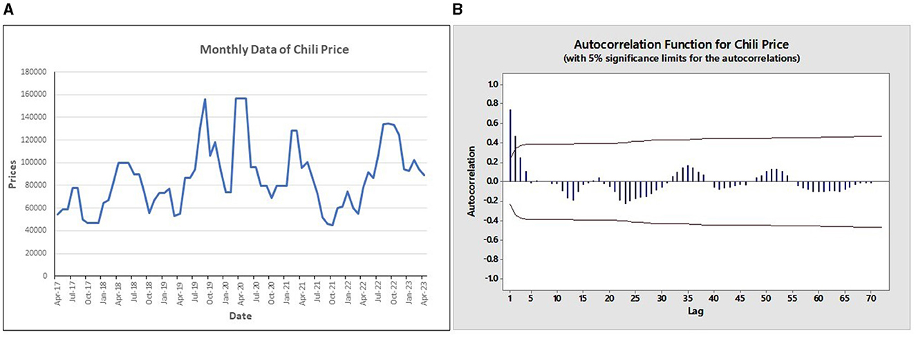
Figure 1. (A) Monthly data plot of chili price and (B) ACF plot of monthly data of chili price.
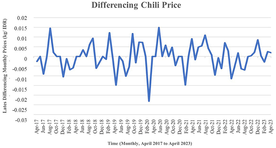
Figure 2. The plot of monthly transformed chili price data after differencing.
Figure 2 shows that the data demonstrated stationarity concerning both the mean and variance. This was evident as the data revealed variations around the mean value while maintaining a constant variance.
The study proceeded to identify the order of autoregressive and moving averages for non-seasonal nonseasonal and seasonal orders before determining the SARFIMA(p, d, q)(P, D, Q)S model. Initially, the nonseasonal order (p, d, q) was determined by examining the results of ACF and PACF plots [29]. The p and q orders could be seen in the PACF and ACF plots, respectively, while d signified the fractional differencing produced using the GPH approach [30]. The following graphic shows the results of the nonseasonal ACF and PACF plots:
Based on Figure 3, the ACF plot was significant at the third lag, indicating that the order was q = 3. Additionally, the PACF plot was also significant at the second lag, indicating that the order was p = 2. The procedure of differencing yielded a value of d = 0.230. Subsequently, the seasonalities of orders P and Q were determined. Figure 1A showed a seasonal effect on the chili price data, implying that a difference on the 12th lag was necessary. The ACF and PACF charts obtained after differencing are shown below:
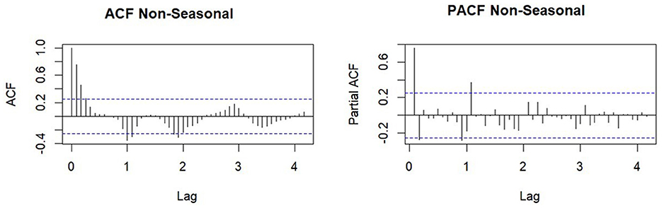
Figure 3. ACF and PACF Plots nonseasonal.
The ACF plot signified significance at the fourth lag, as illustrated in Figure 4, denoting an order of Q = 4 for the seasonal moving average. Moreover, the PACF plot showed significance at the first lag, indicating an order of P = 1 for seasonal autoregressive, along with an order of D=0. In the next step, parameter estimation was carried out for each model. There are six significant SARFIMA models, namely SARFIMA(0, d, 1)(0, 0, 1)12, SARFIMA(0, d, 2)(0, 0, 1)12, SARFIMA(1, d, 2)(0, 0, 1)12, SARFIMA(2, d, 2)(0, 0, 1)12, SARFIMA(0, d, 1)(1, 0, 0)12, and SARFIMA(0, d, 2)(1, 0, 1)12 where the value of d = 0.228. The optimal model was found by comparing the least AIC and BIC values in the table below:
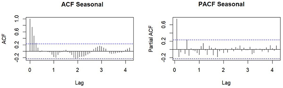
Figure 4. ACF and PACF plots seasonal.
Based on Table 1, SARFIMA(1, 0.228, 2)(0, 0, 1)12 has the smallest value of AIC or BIC that indicates that SARFIMA(1, 0.228, 2)(0, 0, 1)12 is the best model of SARFIMA. The Q-Ljung Box test, which assessed autocorrelation, achieved a p-value of 0.692, exceeding the significance level of 0.05. Similarly, the test for heteroscedasticity produced a p-value of 0.212, which also surpassed the 0.05 significance threshold. In order to test for normality, Jarque-Bera was utilized and it produced a p-value of 0.034, falling below the critical value of 0.05. The result suggested that the data was not normally distributed. However, such deviations were expected in financial data due to price fluctuations. The conclusion was that there was no autocorrelation or heteroscedasticity in the model's residuals, rendering it suitable for use, as depicted in the comparison chart below with the actual data shown in Figure 5.
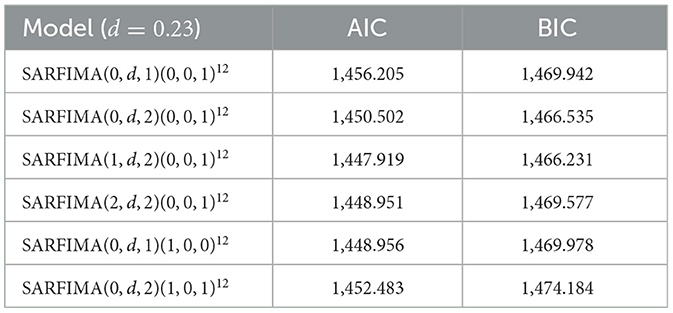
Table 1. AIC and BIC value.
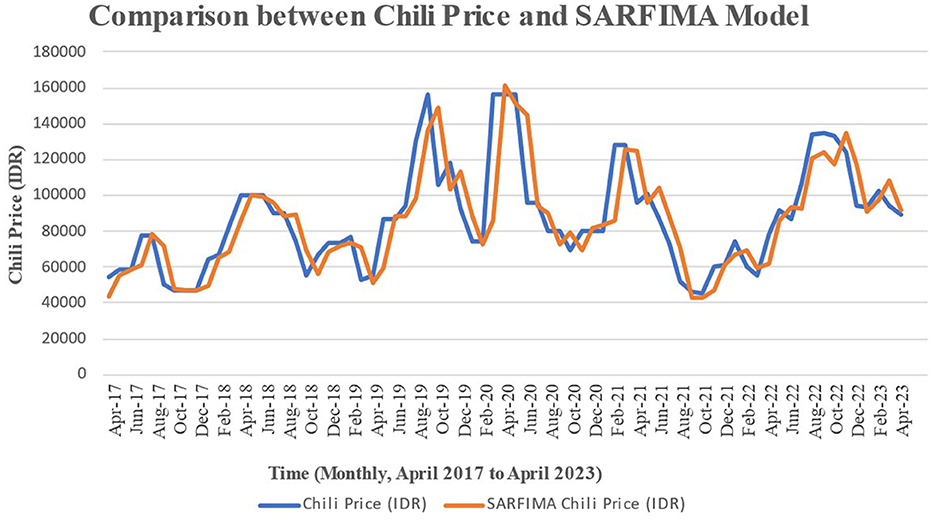
Figure 5. Comparison plot for monthly data of chili price with the SARFIMA model.
In Figure 5, SARFIMA data was in line with the observed data, although discrepancies arose during certain periods, particularly in instances of data increase and decrease. Consequently, the incorporation of exogenous variables into the model became necessary.
The initial step in SARFIMAX modeling consisted of creating a dummy variable for the regression model. This dummy variable comprised Y1, t and Y2, t where Y1, t represented the dummy month of the beginning of the year (January) and Y2, t signified the dummy month of Eid al-Fitr. The dummy variable was selected based on the influence of the increase in chili demand ahead of the Eid al-Fitr holiday. The parameters of the dummy regression model can be calculated as follows:
The significance test for the parameters of the dummy regression model is shown in Table 2.
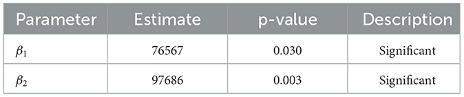
Table 2. Significance test of parameter dummy regression.
In Table 2, each parameter showed significance, indicating that a diagnostic test was conducted on the model's residual data. The test confirmed that the model residuals conformed to the white noise assumption. As a result, the modeling process advanced to SARFIMAX, a fusion of SARFIMA and exogenous variables. The next steps incorporated modeling SARFIMAX, estimating parameters, and identifying the best model. The best model, SARFIMAX(1, d, 2)(0, 0, 1)12 was selected based on the lowest AIC and BIC values. Subsequently, the residual assumptions for the best model included non-autocorrelation, heteroscedasticity, and normality tests, with consecutive p-values of 0.758, 0.054, and 0.126, respectively, which surpassed the significance level of 0.05. The results showed that SARFIMAX(1, d, 2)(0, 0, 1)12 met the assumptions of the residual test and was suitable for use. The comparison chart in Figure 6 shows the model's consistency with actual data.
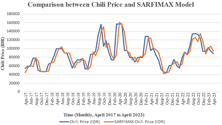
Figure 6. Comparison plot of monthly data of chili price with SARFIMAX model data.
Figure 6 shows that SARFIMAX was in line with the chili price data, due to the incorporation of exogenous variables. This addition significantly minimized modeling errors, indicating that the exogenous variables' substantial influence on chili price sales data fluctuations.
In capturing the error of both the SARFIMA and SARFIMAX models, the following Figure 7 presents the pattern error of both the SARFIMA and SARFIMAX models.
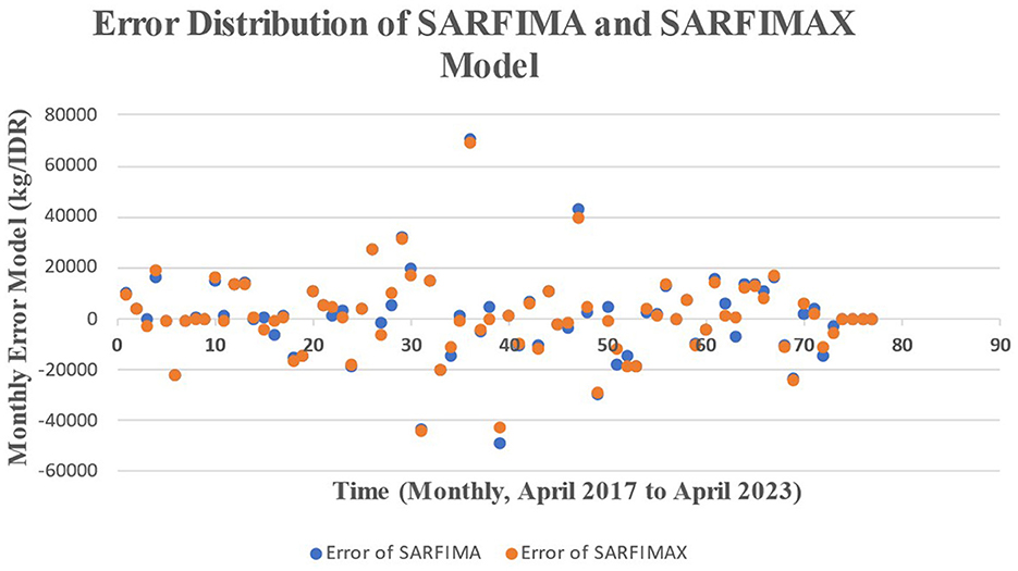
Figure 7. Error distribution of SARFIMA and SARFIMAX models.
Figure 7 shows the error for both the SARFIMA and SARFIMAX models. The errors of both SARFIMA and SARFIMAX models are distributed around zero and do not have a pattern of function. It indicates that the errors for both SARFIMA and SARFIMAX models are random, so the errors for both SARFIMA and SARFIMAX models are distributed in white noise with a mean of zero and constant variance.
In order to improve modeling accuracy, some metrics including MAE, RMSE, and MAPE were applied by using Equation (1), Equation (2), and Equation (3). There are also test statistics of Diebold-Marino (DM), Mean Directional Accuracy (MDA), and coefficient of determination (R2) that are calculated by using Equation (4), Equation (5), and Equation (6), respectively. Table 3 showed the results of chili price data modeling.
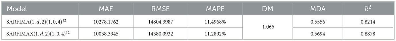
Table 3. The accuracy model evaluation, Diebold-Mariano (DM), and goodness-of-fit (R2).
In both the SARFIMA and SARFIMAX models, the MAPE value remained under 20%, indicating the feasibility of implementing these models. Significantly, SARFIMAX outperformed SARFIMA, showcasing reduced MAE, RMSE, and MAPE values. The addition of exogenous variables in the SARFIMA model reduced errors, indicating the substantial impact of these variables on chili price fluctuations.
In accordance with Table 3, SARFIMA and SARFIMAX have mean directional accuracy (MDA) values of 0.5556 and 0.5694, respectively. The SARFIMA and SARFIMAX models accurately forecast direction changes approximately 55.56% and 56.94% of the time, respectively. In other words, the SARFIMA model has a lower MDA value than the SARFIMAX model, indicating that the SARFIMAX model is slightly better at predicting the direction of change in chili price than the SARFIMA model. The MDA values of SARFIMA and SARFIMAX suggest that the models capture a component of these dynamics but are not highly accurate. This could be due to several factors, including high volatility, supply shocks (natural disasters), variations in demand, political instability, or seasonal production cycles. It may be enabled to enhance its directional accuracy and generate more accurate estimations by including more important features, employing advanced modeling approaches, and significantly adjusting it.
The evaluation of residuals in both SARFIMA and SARFIMAX models was conducted through the Diebold–Mariano (DM) test. Using the significance level of α = 5%, calculations yielded a DM value based on Table 3 is 1.066 which is greater than Zα of 0.832. Moreover, the p-value registered at 0.2900, exceeding the significance level of α = 0.05. This implied that there was no significant difference between these models, as both demonstrated strong goodness-of-fit in tracking chili price movements.
Despite the accuracy model and DM test, there is a goodness-of-fit or determination coefficient (R2) to determine which model is better and closer to 1. Based on Table 3, the goodness-of-fit (R2) of the SARFIMAX model is greater than the SARFIMA model and closer to 1. This means that the SARFIMAX model has better performance in building the chili price model than the SARFIMA model. The determinant coefficients of both SARFIMA and SARFIMAX that are closer to 1 also show that both models have great accuracy. Therefore, the previous data on chili prices can forecast the next period of chili prices precisely.
An examination of the data showed the significant influence of previous data on chili prices, which eventually affected Indonesian inflation. Effective chili price management became very important, given its direct impact on inflation. To achieve this result, the government and stakeholders needed to collaborate in order to improve production. Moreover, the expansion of planting areas and the establishment of appropriate planting schedules ensured consistent chili production.
Exogenous variables, particularly the commencement of the new year and the month preceding the Eid al-Fitr celebration, influenced chili prices. Consequently, chili production planning incorporated these events, considering the high demand for chili driven by various factors, including gastronomic. The seasonal time series model, accounting for long memory and exogenous variables, formed the basis for sustaining chili supply and preserving price stability.
The accuracy model and goodness-of-fit based on Table 3 suggest that the SARFIMA model can be used to demonstrate how the seasonal pattern in the Autoregressive Integrated Moving Average (ARIMA) model evolves with the model's fractional order. The fractional integrated order is frequently applied to demonstrate how long memory pattern data is. It means that data with a significant correlation to previous data is more accurate than integer-order data. Furthermore, the SARFIMA model that is merged with an exogenous variable, also known as SARFIMAX, is a combined model that approaches the actual value more accurately than the original model. It is also used in renewable energy management in sustainable supply chains, where it combines a combination method for choosing appropriate hyperparameters for sub-models and an improved intelligent optimization algorithm [7]. Furthermore, reliable photovoltaics, including wind power generation, implement a combined forecasting system that includes a data preprocessing approach, a sub-predictor selection mechanism, and an optimization strategy with multiple objectives to integrate several forecasting models. The suggested system efficiently combines the benefits of all the algorithms involved, resulting in higher prediction precision and stability. Experiments demonstrated that the suggested system outperforms the comparative systems in terms of point and interval forecasting quality [8].
Extensive studies have been conducted in the fields of time series models, long memory processes, and hybrid time series models. For example, studies have focused on long-term seasonal high-frequency forecasting, using SARFIMA to predict periodic long memory series. Stochastic volatility models, realized using the Gegenbauer long-term memory, have been investigated with the Whittle likelihood estimator to measure realized stochastic volatility [18]. In addition, studies have explored the combination of various time series models, such as the SARFIMA-GARCH, which incorporates seasonal interference to estimate parameters for seasonal level shift SARFIMA (SLS-SARFIMA) and seasonal level shift generalized autoregressive conditional heteroscedasticity (SLS-GARCH) [19]. Other areas of exploration include hybrid long memory modeling and fuzzy time series Markov chains [10] and the hybrid autoregressive integrated moving average model with fuzzy time series Markov chain applied to long memory data [31].
The most common commodity for everyday necessities is chili. The time series method is necessary to identify the pattern in the data since historical data contains a lot of data. Seasonality is a specific occurrence that can be attributed to the national culture or the current season. Since the price of chilies is correlated with its historical price, the best option for constructing the pricing model is to use time series analysis, particularly with respect to ARIMA. Given the robust correlation seen between the current and historical prices, the price of chilies can be categorized as a series data points of with a long memory pattern. Furthermore, Indonesian seasonal variations may also play a role in the production of this item. As a result, the SARFIMA model can be created by modifying the traditional ARIMA model with the influence of long-term memory pattern data and the Indonesian season. In Indonesia, the production of chilies may not be primarily influenced by the season. The production of chili may be impacted by an exogenous variable; hence, the SARFIMA model with its exogenous variable, known as SARFIMAX, is necessary to determine the price of chili.
In conclusion, the ACF plot showed a long-term memory effect in the monthly chili price data, with a gradual and hyperbolic decrease. The results confirmed the presence of a long memory effect in the chili price data, meeting the fractional model criteria. This discovery was further substantiated by the autocorrelation function, which indicated a slow lag decrease for an extended period. Chili data, affected by seasonal factors and exogenous variables, could be effectively modeled using SARFIMAX. The selection of the model was based on a comparison of the AIC and BIC values of various candidates. This selection led to the identification of SARFIMAX(1, d, 2)(0, 0, 1)12 as the optimum model, signifying the enduring influence of previous prices on chili price movements. Finally, the model adeptly captured seasonality, long memory, and exogenous variables, providing a foundation for sustaining chili supply and ensuring price stability. In addition, the SARFIMAX model has maintained the improvement of the accuracy model for better performance and fit.
In this study, the best model of SARFIMAX(1, d, 2)(0, 0, 1)12 is based on the term of season, fractionally integrated order, and exogenous variable that is included in the ARIMA model, ensuring that this proposed model provides the accuracy model precisely and the error model getting smaller than its comparison model of SARFIMA. The seasonal term has been employed to emphasize that chili output is dependent on the season; the fractional integrated order indicates the significance of two sequences of data; and the exogenous variable demonstrates how the Eid al-Fitr event influences chili prices. The accuracy model of the SARFIMAX model has a major impact on reducing errors in the SARFIMA model. The limitation of this study is that the exogenous variable of the new year and the week leading up to Indonesia's Eid al-Fitr celebration can be determined by using A.D. and the Islamic calendar. However, these proposed approaches have limitations if the exogenous variable is an unexpected phenomenon, including high volatility, supply shocks (natural disasters), variations in demand, political instability, or seasonal production cycles. Because of these unexpected behaviors, the commodity price of chili is not always predictable precisely. A dynamic system method is necessary to overcome this chaos effect. In order to improve the accuracy of the model based on the problem of chili productivity, incorporating the term into the SARFIMA model, such as soil fertility as the exogenous variable, may be useful in reducing the model's error and adjusting the assumption error. It could enhance its directional accuracy and generate accurate estimations by including more important factors, employing advanced modeling techniques, and performing significant adjustments.
Publicly available datasets were analyzed in this study. This data can be found here: https://www.bi.go.id/hargapangan.
DD: Conceptualization, Funding acquisition, Supervision, Validation, Writing – review & editing. EW: Data curation, Formal Analysis, Methodology, Writing – original draft. MM: Formal analysis, Methodology, Validation, Writing – review & editing. MY: Methodology, Software, Validation, Visualization, Writing – review & editing.
The author(s) declare that financial support was received for the research, authorship, and/or publication of this article. The authors are grateful to the Ministry of Education, Cultural, Research, and Technology of Indonesia for funding this project, conducted under the scheme of Andalas University's program for research excellence with contract number 012/E5/PG.02.00.PL.2023.
The authors are grateful to the reviewers for their invaluable comments and suggestions, which have significantly contributed to the improvement of the manuscript's quality.
The authors declare that the research was conducted in the absence of any commercial or financial relationships that could be construed as a potential conflict of interest.
All claims expressed in this article are solely those of the authors and do not necessarily represent those of their affiliated organizations, or those of the publisher, the editors and the reviewers. Any product that may be evaluated in this article, or claim that may be made by its manufacturer, is not guaranteed or endorsed by the publisher.
1. Chatfield C, Xing H. The Analysis of Time Series: An Introduction with R. Boca Raton: Chapman and Hall/CRC. (2019). doi: 10.1201/9781351259446
2. Jiang P, Liu Z, Zhang L, Wang J. Advanced traffic congestion early warning system based on traffic flow forecasting and extenics evaluation. Appl Soft Comput. (2022) 118:108544. doi: 10.1016/j.asoc.2022.108544
3. Sun P, Liu Z, Wang J, Zhao W. Interval forecasting for wind speed using a combination model based on multiobjective artificial hummingbird algorithm. Appl Soft Comput. (2024) 150:111090. doi: 10.1016/j.asoc.2023.111090
4. Wang J, Zhang L, Liu Z, Niu X, A. novel decomposition-ensemble forecasting system for dynamic dispatching of smart grid with sub-model selection and intelligent optimization. Expert Syst Appl. (2022) 201:117201. doi: 10.1016/j.eswa.2022.117201
5. Dong Y, Sun Y, Liu Z, Du Z, Wang J. Predicting dissolved oxygen level using Young's double-slit experiment optimizer-based weighting model. J Environ Manage. (2024) 351:119807. doi: 10.1016/j.jenvman.2023.119807
6. Liu Z, Jiang P, De Bock KW, Wang J, Zhang L, Niu X. Extreme gradient boosting trees with efficient Bayesian optimization for profit-driven customer churn prediction. Technol Forecast Soc Change. (2024) 198:122945. doi: 10.1016/j.techfore.2023.122945
7. Sun Y, Ding J, Liu Z, Wang J. Combined forecasting tool for renewable energy management in sustainable supply chains. Comp Indust Eng. (2023) 178:109237. doi: 10.1016/j.cie.2023.109237
8. Zhang L, Wang J, Liu Z. Power grid operation optimization and forecasting using a combined forecasting system. J Forecast. (2023) 42:124–53. doi: 10.1002/for.2888
9. Granger CWJ. Long memory relationships and the aggregation of dynamic models. J Econom. (1980) 14:227–38. doi: 10.1016/0304-4076(80)90092-5
10. Arif E, Devianto D, Yollanda M, Afrimayani A. Analysis of precious metal price movements using long memory and fuzzy time series Markov chain. Int J Energy Econ Policy. (2022) 12:202–14. doi: 10.32479/ijeep.13531
11. Columbu S, Mameli V, Musio M, Dawid P. The Hyvarinen scoring rule in Gaussian linear time series models. J Stat Plan Inference. (2021) 212:126–40. doi: 10.1016/j.jspi.2020.08.004
12. Geweke J, Porter-Hudak S. The estimation and application of long memory time series models. J Time Series Anal. (1983) 4:221–38. doi: 10.1111/j.1467-9892.1983.tb00371.x
13. Monge MUS. historical initial jobless claims. Is it different with the coronavirus crisis? A fractional integration analysis. Int. Econ. (2021) 167:88–95. doi: 10.1016/j.inteco.2020.11.006
14. Bukhari AH, Raja MA, Shoaib M, Kiani AK. Fractional order Lorenz based physic informed SARFIMA-NARX model to monitor and mitigate megacities air pollution. Chaos, Solitons & Fractals. (2022) 161:112375. doi: 10.1016/j.chaos.2022.112375
15. David SA, Inacio Jr CMC, Nunes R, Machado JAT. Fractional and fractal processes applied to cryptocurrencies price series. J Adv Res. (2021) 32:85–98. doi: 10.1016/j.jare.2020.12.012
16. Diongue AK, Diop A, Ndongo M. Seasonal fractional ARIMA with stable innovations. Statist Probab Lett. (2008) 78:1404–11. doi: 10.1016/j.spl.2007.12.011
17. Falatouri T, Darbanian F, Brandtner P, Udokwu C. Predictive analytics for demand forecasting a comparison of SARIMA and LSTM in retail SCM. Procedia Comput Sci. (2022) 200:993–1003. doi: 10.1016/j.procs.2022.01.298
18. Asai M, Mcaler M, Peiris S. Realized stochastic volatility models with generalized Gegenbauer long memory. Economet Statist. (2020) 16:42–54. doi: 10.1016/j.ecosta.2018.12.005
19. Dhliwayo L, Matarise F, Chimedza C. Modelling volatility and level shift in fractionally integrated processes. Novel Res Aspects Mathem Comp Sci. (2022) 1:118–37. doi: 10.9734/bpi/nramcs/v1/2756C
20. Proelss J, Schweizer D, Seiler V. The economic importance of rare earth elements volatility forecasts. Int Rev Financ Analy. (2020) 71:101316. doi: 10.1016/j.irfa.2019.01.010
21. Devianto D, Yollanda M, Maiyastri, Yanuar F. The soft computing FFNN method for adjusting heteroscedasticity on the time series model of currency exchange rate. Front Appl Mathem Statist. (2023) 9:1–18. doi: 10.3389/fams.2023.1045218
22. Wu WZ, Pang H, Zheng C, Xie W, Liu C. Predictive analysis of quarterly electricity consumption via a novel seasonal fractional nonhomogeneous discrete grey model: A case of Hubei in China. Energy. (2021) 229:120714. doi: 10.1016/j.energy.2021.120714
23. Leneenadogo W, Tuaneh GL. Modelling the Nigeria crude oil prices using ARIMA, pre-intervention and post-intervention model. Asian J Probab Statis. (2019) 3:1–12. doi: 10.9734/ajpas/2019/v3i130083
24. Waldman DM, A. note on algebraic equivalence of White's test and a variation of the Godfrey/Breusch-Pagan test for heteroscedasticity. Econ Lett. (1983) 13:197–200. doi: 10.1016/0165-1765(83)90085-X
25. Devianto D, Permana D, Arif E, Afrimayani A, Yanuar F, Maiyastri M, et al. An innovative model for capturing seasonal patterns of train passenger movement using exogenous variables and fuzzy time series hybridization. J Open Innovat: Technol Mark Compl. (2024) 10:100232. doi: 10.1016/j.joitmc.2024.100232
26. Yollanda M, Devianto D, Yozza H. Nonlinear modeling of IHSG with artificial intelligence. IEEE. (2018) 2018:85–90. doi: 10.1109/ICAITI.2018.8686702
27. Bergmeir C, Costantini M, Bentez JM. On the usefulness of cross-validation for directional forecast evaluation. Comp Statist Data Analy. (2014) 76:132–43. doi: 10.1016/j.csda.2014.02.001
28. Denis DJ. Applied Univariate, Bivariate, and Multivariate Statistics: Understanding Statistics for Social and Natural Scientists, with Applications in SPSS and R. New York: Wiley. (2021).
29. Awe O, Okeyinka A, Fatokun JO. An Alternative Algorithm for ARIMA Model Selection. Ayobo: IEEE. (2020). p. 1–4.
30. He C, Kang J, Silvennoinen A, Terasvirta T. Long monthly temperature series and the Vector Seasonal Shifting Mean and Covariance Autoregressive model. J Econom. (2023) 239:105494. doi: 10.1016/j.jeconom.2023.105494
Keywords: seasonality, long memory, exogenous variable, SARFIMA, SARFIMAX, chili price
Citation: Devianto D, Wahyuni E, Maiyastri M and Yollanda M (2024) The seasonal model of chili price movement with the effect of long memory and exogenous variables for improving time series model accuracy. Front. Appl. Math. Stat. 10:1408381. doi: 10.3389/fams.2024.1408381
Received: 28 March 2024; Accepted: 25 June 2024;
Published: 10 July 2024.
Edited by:
V. Venkataramanan, SVKM's Dwarkadas J. Sanghvi College of Engineering, IndiaReviewed by:
Pavan Rayar, SVKM's Dwarkadas J. Sanghvi College of Engineering, IndiaCopyright © 2024 Devianto, Wahyuni, Maiyastri and Yollanda. This is an open-access article distributed under the terms of the Creative Commons Attribution License (CC BY). The use, distribution or reproduction in other forums is permitted, provided the original author(s) and the copyright owner(s) are credited and that the original publication in this journal is cited, in accordance with accepted academic practice. No use, distribution or reproduction is permitted which does not comply with these terms.
*Correspondence: Dodi Devianto, ZGRldmlhbnRvQHNjaS51bmFuZC5hYy5pZA==
Disclaimer: All claims expressed in this article are solely those of the authors and do not necessarily represent those of their affiliated organizations, or those of the publisher, the editors and the reviewers. Any product that may be evaluated in this article or claim that may be made by its manufacturer is not guaranteed or endorsed by the publisher.
Research integrity at Frontiers
Learn more about the work of our research integrity team to safeguard the quality of each article we publish.