Asymmetric generalized error distribution with its properties and applications

The main finding of this study is the derivation of a new probability distribution that reveals interesting properties, especially with various asymmetry and kurtosis behavior. We call this distribution the asymmetric generalized error distribution (AGED). AGED is a new contribution to the field of statistical theory, offering more flexible probability density functions, cumulative distribution functions, and hazard functions than the base distribution. The AGED also includes normal, uniform, Laplace, asymmetric Laplace, and generalized error distribution (GED) as special cases. The mathematical and statistical features of the distribution are derived and discussed. Estimators of the parameters of the distribution are obtained using the maximum likelihood approach. In a simulation study, random samples are generated from the new probability distribution to illustrate what ideal data looks like. Using real data from diverse applications such as health, industry, and cybersecurity domains, the performance of the new distribution is compared to that of other distributions. The new distribution is found to be a better fit for the data, showing great adaptability in the context of real data analysis. We expect the distribution to be applied to many more real data, and the findings of the study can be used as a basis for future research in the field.

1 Introduction

There has been a growing interest in the construction of flexible parametric families of distributions that exhibit asymmetry and peakedness differing from those of symmetric distributions (1–3). Many of these methods center around overcoming the assumptions of normality found in the empirical analysis of many parametric models.

An empirical analysis in various studies suggests that the assumption of normality of real data is often untenable (4, 5), and asymmetry is commonly observed (6, 7). It is highly acknowledged that data with heavy-peaked distribution are encountered in the empirical analysis (8), as is asymmetric distribution (9, 10). In all cases, it is important to adopt a flexible distribution that can directly address asymmetry and peakedness (6, 9).

There has been a different approach to develop asymmetric counterparts of symmetric distributions. Many of these approaches centered on overcoming assumptions of normality (11, 12). In many works of literature, asymmetry is achieved via the transformation of the skewing function (9, 10), which lacks a wide range of skewness and kurtosis. Moreover, the technique of creating asymmetric counterparts of symmetric distributions has a longer history (13–15).

The approach that is commonly considered for constructing classes of asymmetric distributions from symmetric distribution is authored by Azzalini (16, 17). The initial idea appeared in O’hagan and Leonard (18) in the context of base distribution. Azzalini (16, 17) introduced asymmetric distributions called skew-normal (SN). The idea was further extended in Azzalini (13) introduced multivariate asymmetry distributions. An ideal class of distributions obtained from this methodology includes symmetric distributions, mathematical tractability, and a wide range of skewness and kurtosis. The theoretical and statistical properties of the methodology have been studied by various researchers (2, 3, 19, 20).

As noted in (5, 12) the generalized error distribution (GED) has short tails, making it unsuitable for modeling data with heavier tails. One method to solve this problem, as suggested in Azzalini (16), is to use an asymmetric pdf with flexible tails and excess kurtosis. Azzalini’s methodology generates distributions with flexible tails and excess kurtosis.

In this study, we follow Azzalini’s methodology to introduce a new distribution that is flexible enough for modeling data with heavier tails and excess kurtosis. More data with heavier tails and excess kurtosis are adequately modeled to the distribution and play an important role in this context. This new distribution is called asymmetric generalized error distribution (AGED) and is denoted by $\left\{AGED\left(\alpha \right):\alpha ϵℝ\right\}$, where $\alpha$ represents the asymmetry parameter so that $AGED\left(\alpha =0\right)$ corresponds to the generalized error distribution. We outline some properties of the distribution, provide a graphical representation of the distribution, and discuss some inferences.

2 Generalized error distribution

The GED is a symmetric and unimodal member of the exponential family of distribution introduced by Subbotin (22) and has been used by different authors with different parameterizations (23, 24). A random variable $X$ have a generalized error distribution if its probability density function (pdf) is expressed by (21):

$\begin{array}{ll}g\left(x;\mu ,\sigma ,\beta \right)=\frac{1}{2^{1+1/\beta }\sigma \Gamma \left(1+1/\beta \right)}\exp \left(-\frac{1}{2}{\left|\frac{x-\mu }{\sigma }\right|}^{\beta }\right)& (1)\end{array}$

where $\mu \in ℝ$ is the location parameter, $\sigma \in {ℝ}^{+}$ is the scale parameter, and $\beta \in {ℝ}^{+}$ is the shape parameter. Here, $\Gamma (.)$ is the Euler gamma function. We denote it by $X~GED\left(x;\mu ,\sigma ,\beta \right)$.

It is convenient to work with the alternative expression given in Eq. 1, which allows for mean zero and variance unity (25). The variance of the GED is a function of $\beta$ (26, 27). To rescale its variance, a scaling parameter η is introduced, and a substitution is made for $\sigma \to \sigma {\eta }^{1/\beta }$ in Eq. 1 to get the following equivalent pdf (25):

$\begin{array}{ll}g\left(x;\mu ,\sigma ,\beta \right)=\frac{1}{2^{1+1/\beta }\sigma {\eta }^{1/\beta }\Gamma \left(1+1/\beta \right)}\exp \left(-\frac{1}{2\eta }{\left|\frac{x-\mu }{\sigma }\right|}^{\beta }\right)& (2)\end{array}$

Or

$\begin{array}{l}g\left(x;\mu ,\sigma ,\beta \right)={\left\{\frac{\Gamma \left(3/\beta \right)}{\Gamma \left(1/\beta \right)}\right\}}^{\frac{1}{2}}\frac{1}{2\sigma \Gamma \left(1+1/\beta \right)}\\ \exp \left(-{\left\{\frac{\Gamma \left(3/\beta \right)}{\Gamma \left(1/\beta \right)}{\left(\frac{x-\mu }{\sigma }\right)}^2\right\}}^{\frac{\beta }{2}}\right)\end{array}\text{ (3)}$

3 The newly suggested asymmetric generalized error distribution

In this section, the method of generating an asymmetric distribution from a symmetric distribution is presented to develop the new asymmetric generalized error distribution (AGED). Here, the method of constructing classes of asymmetric distributions suggested by Azzalini (16, 17) is used. The authors introduced a methodology that can be used to derive an asymmetric distribution from an existing symmetric distribution. This is expressed in Proposition 1.

3.1 Proposition 1

Let $\varphi \left(x\right)$ and $\Phi \left(x\right)$ be pdf and cdf of the random variable $X$, respectively, and characterizing symmetric distribution such that $\varphi \left(-x\right)=\varphi \left(x\right)$, $\Phi \left(-x\right)=1-\Phi \left(x\right)$, for all $x\in ℝ$. Then, the random variable $X$ has an asymmetric probability density function expressed in the form of:

$\begin{array}{ll}f\left(x;\alpha \right)=2\varphi \left(x\right)\Phi \left(\alpha x\right)& (4)\end{array}$

where $\alpha \in ℝ$ is the asymmetry parameter and $f\left(x\right)$ is an asymmetric version of a symmetric base pdf.

In this study, we derived a new asymmetric distribution called the AGED. The approach of Azzalini (16, 17) is used with the base distribution of the generalized error distribution in Eq. 3.

3.2 Theorem 1

For the generalized error distribution, GED, in Eq. 3, the new asymmetric generalized error distribution (AGED), has probability density and cumulative distribution functions expressed as follows:

$\begin{array}{l}f\left(x;\alpha \right)=2g\left(x\right)G\left(\alpha x\right)\\ =\{\begin{array}{c}\begin{array}{l}2\frac{{\left(k\left(\beta \right)\right)}^2}{\beta }{\left(\frac{\Gamma \left(3/\beta \right)}{\Gamma \left(1/\beta \right)}\right)}^{\frac{1}{2}}\exp \left(-{\left\{\frac{\Gamma \left(3/\beta \right)}{\Gamma \left(1/\beta \right)}{\left(\frac{x-\mu }{\sigma }\right)}^2\right\}}^{\frac{\beta }{2}}\right)\\ \Gamma \left(\frac{1}{\beta },\alpha z\right),x\le \mu \end{array}\\ \begin{array}{l}2k\left(\beta \right){\left(\frac{\Gamma \left(3/\beta \right)}{\Gamma \left(1/\beta \right)}\right)}^{\frac{1}{2}}\exp \left(-{\left\{\frac{\Gamma \left(3/\beta \right)}{\Gamma \left(1/\beta \right)}{\left(\frac{x-\mu }{\sigma }\right)}^2\right\}}^{\frac{\beta }{2}}\right)\\ \left\{1-\frac{k\left(\beta \right)}{\beta }\Gamma \left(\frac{1}{\beta },\alpha z\right)\right\},x>\mu \end{array}\end{array}\text{ (5)}\end{array}$

$F\left(x;\alpha \right)=2{\displaystyle \underset{-\infty }{\overset{x}{\int }}}g\left(t\right)G\left(\alpha t\right)dt$

$=\{\begin{array}{l}\frac{\mathrm{k}\left(\beta \right)}{\beta }\Gamma \left(\frac{1}{\beta },\alpha z\right)-\frac{1}{2\pi }{\displaystyle \underset{0}{\overset{\tau }{\int }}}\frac{\exp \left(-{\alpha }^2\left(1+{\mathrm{x}}^2\right)/2\right)}{1+{\mathrm{x}}^2}\text{dx},\mathrm{x}\le \mu \\ 1-\frac{\mathrm{k}\left(\beta \right)}{\beta }\Gamma \left(\frac{1}{\beta },\alpha z\right)-\frac{1}{2\pi }{\displaystyle \underset{0}{\overset{\tau }{\int }}}\frac{\exp \left(-{\alpha }^2\left(1+{\mathrm{x}}^2\right)/2\right)}{1+{\mathrm{x}}^2}\text{dx},\mathrm{x}>\mu \end{array}\text{ (6)}$

where $k\left(\beta \right)=\frac{1}{2\sigma \Gamma \left(1+1/\beta \right)}$, $\frac{1}{2\pi }{\displaystyle \underset{0}{\overset{\tau }{\int }}}\frac{\exp \left(-{\alpha }^2\left(1+x^2\right)/2\right)}{1+x^2}dx=T\left(x,\alpha \right)$ and $T(.)$ is Owen’s $T$ function (28). Here, Γ$(.)$ is the Euler gamma function. The parameters $\alpha$ determine the degree of asymmetry, which can generate distributions with flexible tail behavior and excess kurtosis. We denote it by $X~AGED\left(\mu ,\sigma ,\beta ,\alpha \right)$. See Ref. (29–31).

3.3 Proof

Suppose $g\left(x\right)$ is a pdf of GED defined in Eq. 3 and cdf, $G\left(\alpha x\right)$ obtained as:

$\begin{array}{l}G\left(\alpha x\right)=P\left(X\le \alpha x\right)={\displaystyle \underset{-\infty }{\overset{\alpha x}{\int }}}g\left(x;\mu ,\sigma ,\beta \right)dx\\ \begin{array}{l}={\displaystyle \underset{-\infty }{\overset{\alpha x}{\int }}}{\left\{\frac{\Gamma \left(3/\beta \right)}{\Gamma \left(1/\beta \right)}\right\}}^{\frac{1}{2}}\frac{1}{2\sigma \Gamma \left(1+1/\beta \right)}\\ \exp \left(-{\left\{\frac{\Gamma \left(3/\beta \right)}{\Gamma \left(1/\beta \right)}{\left(\frac{x-\mu }{\sigma }\right)}^2\right\}}^{\frac{\beta }{2}}\right)dx\end{array}\end{array}\text{ (7)}$

We have two cases to consider.

Case 1: for $x\le \mu$

Let, $\begin{array}{l}z={\left\{\frac{\Gamma \left(3/\beta \right)}{\Gamma \left(1/\beta \right)}{\left(\frac{x-\mu }{\sigma }\right)}^2\right\}}^{\frac{\beta }{2}}\Rightarrow \\ dx=-\frac{dz}{\beta \times z^{1-\frac{1}{\beta }}\frac{\Gamma \left(3/\beta \right)}{\Gamma \left(1/\beta \right)}\ast {\left(\frac{\Gamma \left(1/\beta \right)}{\Gamma \left(3/\beta \right)}\right)}^{1/2}}\end{array}$

$\begin{array}{l}G\left(\alpha x\right)={\displaystyle \underset{-\infty }{\overset{\alpha x}{\int }}}{\left\{\frac{\Gamma \left(3/\beta \right)}{\Gamma \left(1/\beta \right)}\right\}}^{\frac{1}{2}}\frac{1}{2\sigma \Gamma \left(1+1/\beta \right)}\\ \exp \left(-{\left\{\frac{\Gamma \left(3/\beta \right)}{\Gamma \left(1/\beta \right)}{\left(\frac{x-\mu }{\sigma }\right)}^2\right\}}^{\frac{\beta }{2}}\right)dx\end{array}\text{ (8)}$

$=\frac{{\left(\frac{\Gamma \left(3/\beta \right)}{\Gamma \left(1/\beta \right)}\right)}^{1/2}}{\frac{\Gamma \left(3/\beta \right)}{\Gamma \left(1/\beta \right)}\ast {\left(\frac{\Gamma \left(1/\beta \right)}{\Gamma \left(3/\beta \right)}\right)}^{1/2}2\beta \sigma \Gamma \left(1+1/\beta \right)}{\displaystyle \underset{\alpha z}{\overset{\infty }{\int }}}{z}^{\frac{1}{\beta }-1}\exp \left(-z\right)dz$

$\begin{array}{ll}=\frac{1}{2\beta \sigma \Gamma \left(1+1/\beta \right)}\Gamma \left(\frac{1}{\beta },\alpha z\right)& (9)\end{array}$

Case 2: for $x>\mu$, similarly

$\begin{array}{l}G\left(\alpha x\right)={\displaystyle \underset{-\infty }{\overset{\alpha x}{\int }}}{\left\{\frac{\Gamma \left(3/\beta \right)}{\Gamma \left(1/\beta \right)}\right\}}^{\frac{1}{2}}\frac{1}{2\sigma \Gamma \left(1+1/\beta \right)}\\ \exp \left(-{\left\{\frac{\Gamma \left(3/\beta \right)}{\Gamma \left(1/\beta \right)}{\left(\frac{x-\mu }{\sigma }\right)}^2\right\}}^{\frac{\beta }{2}}\right)dx\end{array}$

$=1-\frac{{\left(\frac{\Gamma \left(3/\beta \right)}{\Gamma \left(1/\beta \right)}\right)}^{1/2}}{\frac{\Gamma \left(3/\beta \right)}{\Gamma \left(1/\beta \right)}\ast {\frac{\Gamma \left(1/\beta \right)}{\Gamma \left(3/\beta \right)}}^{1/2}2\beta \sigma \Gamma \left(1+1/\beta \right)}{\displaystyle \underset{\alpha z}{\overset{\infty }{\int }}}{z}^{\frac{1}{\beta }-1}\exp \left(-z\right)dz$

$\begin{array}{ll}=1-\frac{1}{2\beta \sigma \Gamma \left(1+1/\beta \right)}\Gamma \left(\frac{1}{\beta },\alpha z\right)& (10)\end{array}$

3.4 Corollary 1

A linear combination of the AGED is also asymmetric. In particular, the inclusion of $\mu$ and variance ${\sigma }^2$ is possible using the transformation, $Y=\mu +\sigma X$, where $X$ have AGED with mean zero and variance 1. Then, a random variable $Y$ is said to have an asymmetric generalized error distribution, $Y~AGED\left(\mu ,\sigma ,\beta ,\alpha \right)$, and it has pdf expressed by:

$\begin{array}{ll}f\left(y;\alpha \right)=2g\left(\frac{y-\mu }{\sigma }\right)G\left(\alpha \frac{y-\mu }{\sigma }\right)& (11)\end{array}$

Where $g(.)$ and $G(.)$ are the pdf and cdf of the symmetric base distribution, respectively, $\alpha$ is the asymmetry parameters, and $f(.)$ is the asymmetric version made from the symmetric distribution.

The theorem 2 shows a pdf of the AGED with shape parameter $\beta$ and asymmetry parameter $\alpha$, which is generated using the representation given in Eq. 12.

3.5 Theorem 2

Let $U$ and $V$ be symmetric random variables such that $U~GED\left(\mu ,\sigma ,\beta \right)$ and $V~N\left(\mu ,\sigma \right)$. Then, the representation of the new asymmetric generalized error distribution is

$\begin{array}{ll}X=U|\left[V\le \alpha U\right]& (12)\end{array}$

We call the distribution of $X$ the asymmetric generalized error distribution (AGED).

3.6 Proof

Let $X=U|V\le \alpha U.$ Then

$P\left(X\le x\right)=P\left(U|V\le \alpha U\le x\right)$

$\begin{array}{ll}=\frac{P\left(U\le x,V\le \alpha U\right)}{P\left(V\le \alpha U\right)}& (13)\end{array}$

But, $U$ and $V$ are symmetric random variables, and following that:

$P\left(U\le x,V\le \alpha u\right)={\displaystyle \underset{-\infty }{\overset{\alpha u}{\int }}}{\displaystyle \underset{-\infty }{\overset{x}{\int }}}g\left(u\right)g\left(v\right)dudv$

$\begin{array}{ll}={\displaystyle \underset{-\infty }{\overset{x}{\int }}}g\left(u\right)G\left(\alpha u\right)du& (14)\end{array}$

Since $U$ and $V$ have symmetric pdf, we have:

$\begin{array}{ll}P\left(V\le \alpha U\right)=\frac{1}{2}& (15)\end{array}$

$P\left(X\le x\right)={\displaystyle \underset{-\infty }{\overset{x}{\int }}}g\left(u\right)G\left(\alpha u\right)du$

$\begin{array}{ll}={\displaystyle \underset{-\infty }{\overset{x}{\int }}}2g\left(u\right)G\left(\alpha u\right)du& (16)\end{array}$

Then, $X$ has a pdf of $2g(.)G(.)$, which is defined in Eq. 5.

3.7 Corollary 2

Let $X~AGED\left(\mu ,\sigma ,\beta ,\alpha \right)$ and $X=U|V\le \alpha U$, where $U~GED\left(\mu ,\sigma ,\beta \right)$ and $V~N\left(\mu ,\sigma \right)$. Then, for $\alpha \to 0$, random variable $X$ converges in distribution to $U$.

3.8 Proof

Since $V~N\left(\mu ,\sigma \right)$ and $E{\left(V-c\right)}^2\to 0$, that is $V\stackrel{P}{\to }c$. Therefore, by applying Slutsky’s lemma (32) to $X=U|V\le \alpha U$ to obtain:

$X\stackrel{d}{\to }U~GED\left(\mu ,\sigma ,\beta \right),\alpha \to 0$

That is, for decreasing value of $\alpha$, $X$ converges in distribution to $GED\left(\mu ,\sigma ,\beta \right)$.

Using the distribution, reliability measures can be assessed. Identification of a system’s important components and estimation of the effects of component failure are important in reliability measures (33). Therefore, it is essential to derive the functions of the AGED reliability measures, an important quantity characterizing life phenomena (34).

For a random variable $X$ with probability density function and cumulative distribution function $f\left(x\right)$ and $F\left(x\right)$ defined in Eqs 5, 6, respectively, survival and hazard functions can be defined as $S\left(x\right)=1-F\left(x\right)$ and $h\left(x\right)=f\left(x\right)/S\left(x\right)$, respectively (35).

4 Plots of the asymmetric generalized error distribution

Graphs of probability density and cumulative distribution function of AGED are illustrated in Figure 1 for some values of parameters that give possible shapes of function. The asymmetry parameter $\alpha$ controls the magnitude of the asymmetry exhibited by the probability density function. The AGED can take a number of forms, including symmetric, near symmetric, and asymmetric. As $\alpha \to +\infty$, the asymmetric generalized error distribution converges in distribution to the half asymmetric generalized error distribution, and for $\alpha \to 0$, the distribution reduced to the generalized error distribution. However, for $\alpha =0.5$, the generalized error distribution converges to the asymmetric generalized error distribution (Figure 2).

Figure 1

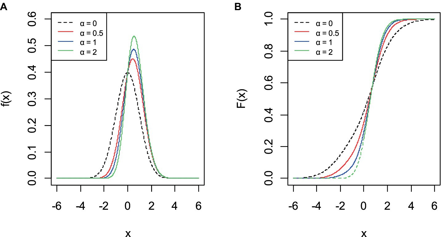
Figure 1. Graph of probability density (A) and cumulative distribution function (B) of AGED.

Figure 2

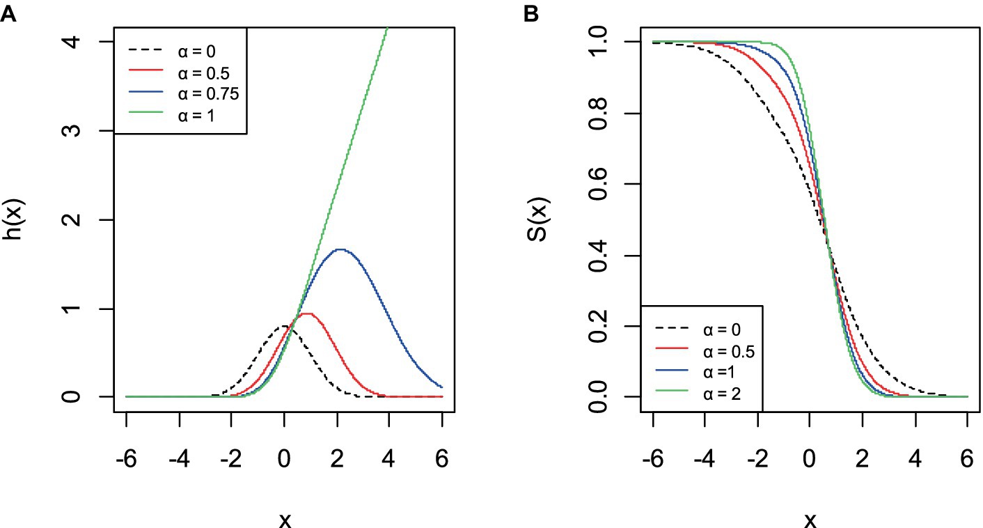
Figure 2. Graph of survival function (B) and hazard function (A) of AGED.

Extremely illustrated properties instantly follow from definition 1 and Figure 1 is as follows:

If $X~AGED\left(\mu ,\sigma ,\beta ,\alpha \right)$, then the following properties are concluded directly from theorem (1) and Figures 1, 3, 4:

• If $\alpha =0$, then $X~GED\left(\mu ,\sigma ,\beta \right)$: The distribution reduced to the generalized error distribution with location parameter $\mu$, scale parameter $\sigma$, and shape parameter $\beta$ (21).

• If $\alpha \to \infty$, then $X~HAGED\left(\mu ,\sigma ,\beta ,\alpha \right)$: The distribution becomes a half asymmetric generalized error distribution with location parameter $\mu$, scale parameter $\sigma$, and shape parameter $\beta$.

• If $\alpha =0.5$ and $\beta =$1, then $X~ALap\left(\mu ,\sigma ,\beta \right)$: The distribution is asymmetric Laplace distribution with location parameter $\mu$ and scale parameters $\sigma$ and $\beta$ (27).

• If $\alpha =2$, then $X~AST\left(\alpha \right)$: The AGED distribution goes to asymmetric student $t-$ distribution with location parameter $\mu$, scale parameter $\sigma$, and shape parameters $\alpha$ and $\beta$ (26).

Figure 3

Figure 3. Graph of the density function of AGED with different values of parameters.

Figure 4

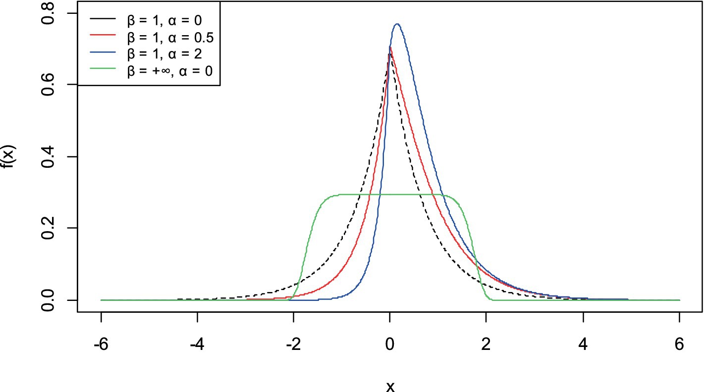
Figure 4. Graph of density functions of AGED for different values of parameters.

5 Moment and its measures

Let $X$ be a random variable from AGED with pdf defined in Eq. 5, the $r^{\prime }th$ moments of the random variable $X$ is obtained as follows (36):

${\pi }_r=E\left[X^r\right]={\displaystyle \underset{-\infty }{\overset{\infty }{\int }}}{x}^{r}2g\left(x\right)G\left(\alpha x\right)dx$

$\begin{array}{l}={\displaystyle \underset{-\infty }{\overset{\infty }{\int }}}2x^{r}G\left(\alpha x\right)\times {\left\{\frac{\Gamma \left(3/\beta \right)}{\Gamma \left(1/\beta \right)}\right\}}^{\frac{1}{2}}\frac{1}{2\sigma \Gamma \left(1+1/\beta \right)}\\ \exp \left(-{\left\{\frac{\Gamma \left(3/\beta \right)}{\Gamma \left(1/\beta \right)}{\left(\frac{x-\mu }{\sigma }\right)}^2\right\}}^{\frac{\beta }{2}}\right)dx\end{array}$

$\begin{array}{ll}=E\left[2X_g^{r}G\left(\alpha X_g\right)\right]& (17)\end{array}$

where $X_g~GED\left(\mu ,\sigma ,\beta \right)$. However, for a random variable $X~AGED\left(\mu ,\sigma ,\beta ,\alpha \right)$ with pdf given in Eq. 5, it follows the form of the binomial theorem:

${\pi }_r=E\left[X^r\right]=E\left[{\left(\mu +\sigma Z\right)}^r\right]$

$={\displaystyle \sum _{k=0}^r}\left(\begin{array}{c}r\\ k\end{array}\right){\mu }^{r-k}{\sigma }^{k}E\left[Z^k\right]\text{ (18)}$

Consider a random variable $Z~AGED\left(0,1,\beta ,\alpha \right)$ with pdf in Eq. 5, then

$\begin{array}{l}E\left[Z^k\right]={\displaystyle \underset{-\infty }{\overset{\infty }{\int }}}{z}^k{\left\{\frac{\Gamma \left(3/\beta \right)}{\Gamma \left(1/\beta \right)}\right\}}^{\frac{1}{2}}\frac{2}{2\Gamma \left(1+1/\beta \right)}\exp \left(-z^{\beta }\right)G\left(\alpha z\right)dz\\ ={\displaystyle \underset{0}{\overset{\infty }{\int }}}{z}^k{\left\{\frac{\Gamma \left(3/\beta \right)}{\Gamma \left(1/\beta \right)}\right\}}^{\frac{1}{2}}\frac{2}{2\Gamma \left(1+1/\beta \right)}\exp \left(-z^{\beta }\right)G\left(\alpha z\right)dz\\ +{\left(-1\right)}^k{\displaystyle \underset{0}{\overset{\infty }{\int }}}{z}^k{\left\{\frac{\Gamma \left(3/\beta \right)}{\Gamma \left(1/\beta \right)}\right\}}^{\frac{1}{2}}\frac{2}{2\Gamma \left(1+1/\beta \right)}\exp \left(-z^{\beta }\right)G\left(-\alpha z\right)dz\\ =E_1+E_2\end{array}\text{ (19)}$

$\begin{array}{l}{E}_1={\displaystyle \underset{0}{\overset{\infty }{\int }}}{\left(\frac{\Gamma \left(3/\beta \right)}{\Gamma \left(1/\beta \right)}\right)}^{\frac{1}{2}}\frac{2}{2\Gamma \left(1+1/\beta \right)}\exp \left(-z^{\beta }\right)G\left(\alpha z\right)dz\\ =\frac{2\Gamma \left[\left(k+1\right)/\beta \right]}{2\beta \Gamma \left(1+1/\beta \right)}E\left[G\left(\alpha W^{1/\beta }\right)\right]& (20)\end{array}$

where $W=z^{\beta }$ and similarly,

$E_2={\left(-1\right)}^K{\displaystyle \underset{0}{\overset{\infty }{\int }}}{z}^k{\left(\frac{\Gamma \left(3/\beta \right)}{\Gamma \left(1/\beta \right)}\right)}^{\frac{1}{2}}\frac{2}{2\Gamma \left(1+1/\beta \right)}\exp \left(-z^{\beta }\right)G\left(-\alpha z\right)dz$

$\begin{array}{l}={\left(-1\right)}^K{\displaystyle \underset{0}{\overset{\infty }{\int }}}\frac{W^{k/\beta }}{\beta w^{1-1/\beta }}{\left(\frac{\Gamma \left(3/\beta \right)}{\Gamma \left(1/\beta \right)}\right)}^{\frac{1}{2}}\frac{2}{2\Gamma \left(1+1/\beta \right)}\\ \exp \left(-w\right)G\left(-\alpha W^{1/\beta }\right)dw\end{array}$

$\begin{array}{ll}={\left(-1\right)}^K\frac{2\Gamma \left[\left(k+1\right)/\beta \right]}{2\beta \Gamma \left(1+1/\beta \right)}E\left[1-G\left(\alpha W^{1/\beta }\right)\right]& (21)\end{array}$

and $k^{\prime }th$ moment of $Z$ becomes:

$E\left[Z^k\right]=\frac{\Gamma \left[\left(k+1\right)/\beta \right]}{\beta \Gamma \left[1+1/\beta \right]}\left\{E\left[G\left(\alpha W^{1/\beta }\right)+{\left(-1\right)}^{k}E\left(1-G\left(\alpha W^{1/\beta }\right)\right)\right]\right\}$

$=\{\begin{array}{l}\frac{\Gamma \left[\left(k+1\right)/\beta \right]}{\beta \Gamma \left[1+1/\beta \right]}ifkeven\\ \frac{\Gamma \left[\left(k+1\right)/\beta \right]}{\beta \Gamma \left[1+1/\beta \right]}\left\{2E\left[G\left(\alpha W^{1/\beta }\right)\right]-1\right\}ifkodd\end{array}\text{ (22)}$

Therefore, for a random variable $X~AGED\left(\mu ,\sigma ,\beta ,\alpha \right)$, the $r^{\prime }th$ moment for a random variable $X$ can be defined as:

$\begin{array}{l}E\left[X^r\right]={\mu }^r{\displaystyle \sum _{k=0}^r}\left(\begin{array}{c}r\\ k\end{array}\right){\left(\frac{\sigma }{\mu }\right)}^k\frac{\Gamma \left[\left(k+1\right)/\beta \right]}{\beta \Gamma \left[1+1/\beta \right]}\\ \left\{E\left[G\left(\alpha W^{1/\beta }\right)\right]+{\left(-1\right)}^{k}E\left[1-G\left(\alpha W^{1/\beta }\right)\right]\right\}\end{array}\text{ (23)}$

In particular, the first four moments of a random variable $X$ are defined as:

${\pi }_1=E\left[X\right]=\mu +\sigma E\left[Z\right]$

${\pi }_2=E\left[X^2\right]={\mu }^2+2\mu \sigma E\left[Z\right]+{\sigma }^{2}E\left[Z^2\right]$

${\pi }_3=E\left[X^3\right]={\mu }^3+3{\mu }^2\sigma E\left[Z\right]+3\mu {\sigma }^{2}E\left[Z^2\right]+{\sigma }^{3}E\left[Z^3\right]$

$\begin{array}{l}{\pi }_4=E\left[X^4\right]={\mu }^4+4{\mu }^3\sigma E\left[Z\right]+6{\mu }^2{\sigma }^{2}E\left[Z^2\right]\\ +4\mu {\sigma }^{3}E\left[Z^3\right]+{\sigma }^{4}E\left[Z^4\right]\end{array}$

The skewness and kurtosis of the asymmetric generalized error distribution are functions of $\mu ,\sigma ,\beta$, and $\alpha$. However, the actual equations in terms of $\mu ,\sigma ,\beta$, and $\alpha$ are quite expansive. In compact form, we can write the variance $\left(\omega \right)$, skewness $\left({\gamma }_3\right)$, and kurtosis $\left({\gamma }_4\right)$ of $X$ using the standardized moments of $Z$ and defined as:

$\omega ={\sigma }^2\left[E\left[Z^2\right]-{\left(E\left[Z\right]\right)}^2\right]$

${\gamma }_3=\frac{E{\left[\sigma Z-E\left(\sigma Z\right)\right]}^3}{{\left(E{\left[\sigma Z-E\left(\sigma Z\right)\right]}^2\right)}^{\frac{3}{2}}}$

${\gamma }_4=\frac{E{\left[\sigma Z-E\left(\sigma Z\right)\right]}^4}{{\left(E{\left[\sigma Z-E\left(\sigma Z\right)\right]}^2\right)}^2}$

We perform a brief comparison illustrating that the tails of the AGED are heavier than those of the GED. Table 1 noted that the AGED has much heavier tails than the GED, as Figure 1 depicts the AGED for different values of parameters.

Table 1

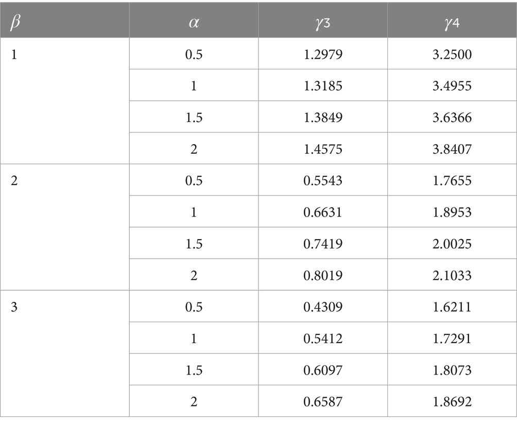
Table 1. The skewness $\left({\gamma }_3\right)$ and kurtosis coefficient $\left({\gamma }_4\right)$ of AGED for selected values of parameters.

Similarly, the degree of asymmetry and peakedness of the AGED for different values of $\beta$ and $\alpha$ are shown, and for small values of $\beta$, the kurtosis coefficient increases in the AGED. The ranges of both coefficients are smaller in GED. Thus, the AGED is more flexible for modeling data with larger coefficients of asymmetry and kurtosis.

6 Estimation of the parameters

In this section, we go over how to estimate the AGED parameters using the maximum likelihood approach.

6.1 Maximum likelihood estimation

Let $X_1,X_2,\cdots ,X_n$ be an independent and identically distributed (i.i.d.) random variable and $X_i$ having the density function $AGED\left(\mu ,\sigma ,\beta ,\alpha \right)$ defined in Eq. 5, then the likelihood function of AGED is defined as (36):

$\begin{array}{ll}{\Lambda }_n\left(\theta \right)={\displaystyle \prod _{i=1}^n}f\left(X_i;\theta \right)& (24)\end{array}$

The maximum likelihood estimator is the value $\theta$ that maximizes the likelihood function (36). Rather than the likelihood function, the log-likelihood function of AGED is given as:

$\begin{array}{ll}{\mathcal{L}}_n\left(\theta |x_i\right)=nln\left(2\right)+{\displaystyle \sum _{i=1}^n}lng\left(\frac{x_i-\mu }{\sigma }\right)+{\displaystyle \sum _{i=1}^n}lnG\left(\alpha \frac{x_i-\mu }{\sigma }\right)& (25)\end{array}$

where $\ln (.)$ is the natural logarithm function, and $\theta =\left(\mu ,\sigma ,\beta ,\alpha \right)$.

By differentiating Eq. 25 with respect to the parameters $\mu ,\sigma ,\beta ,$ and $\alpha$ and equating them to 0, we obtain:

$\begin{array}{ll}\frac{\partial {\mathcal{L}}_n^{\prime }\left(\theta \right)}{\partial \mu }=\frac{\beta }{\sigma }{\displaystyle \sum _{i=1}^n}-\frac{1}{2}{\left(\frac{x_i-\mu }{\sigma }\right)}^{\beta -1}-\frac{\alpha }{\sigma }{\displaystyle \sum _{i=1}^n}\frac{g\left(\alpha \frac{x_i-\mu }{\sigma }\right)}{G\left(\alpha \frac{x_i-\mu }{\sigma }\right)}=0& (26)\end{array}$

$\begin{array}{l}\frac{\partial {\mathcal{L}}_n^{\prime }\left(\theta \right)}{\partial \sigma }=-\frac{n}{\sigma }-\frac{1}{2}\beta {\displaystyle \sum _{i=1}^n}\left(\frac{x_i-\mu }{{\sigma }^2}\right){\left(\frac{x_i-\mu }{\sigma }\right)}^{\beta -1}\\ -{\displaystyle \sum _{i=1}^n}\alpha \left(\frac{x_i-\mu }{{\sigma }^2}\right)\frac{g\left(\alpha \frac{x_i-\mu }{\sigma }\right)}{G\left(\alpha \frac{x_i-\mu }{\sigma }\right)}=0\end{array}\text{ (27)}$

$\begin{array}{l}\frac{\partial {\mathcal{L}}_n^{\prime }\left(\theta \right)}{\partial \beta }=-n\left(\frac{\ln \left(2\right)}{{\beta }^2}+\frac{n{\Gamma }^{\prime }\left(1+1/\beta \right)}{\Gamma \left(1+1/\beta \right)}\right)\\ +\frac{1}{2}{\displaystyle \sum _{i=1}^n}{\left(\frac{x_i-\mu }{\sigma }\right)}^{\beta }\ln \left(\frac{x_i-\mu }{\sigma }\right)=0\end{array}\text{ (28)}$

$\begin{array}{ll}\frac{\partial {\mathcal{L}}_n^{\prime }\left(\theta \right)}{\partial \alpha }={\displaystyle \sum _{i=1}^n}\left(\frac{x_i-\mu }{\sigma }\right)\frac{g\left(\alpha \frac{x_i-\mu }{\sigma }\right)}{G\left(\alpha \frac{x_i-\mu }{\sigma }\right)}=0& (29)\end{array}$

Solving Eqs 26–29, we get MLEs of $\mu ,\sigma ,\beta ,$ and $\alpha$. However, there is no explicit form for the solutions to these equations; thus, we obtain the MLEs numerically using the fitdistrplus package in R (37).

Maximum likelihood estimators are consistent in the sense that ${\hat{\theta }}_n\stackrel{p}{\to }\theta$ as $n\to \infty$ and asymptotically normally distributed: such that $\sqrt{n}\left|{\hat{\theta }}_n-\theta \right|\stackrel{d}{\to }{N}_4\left(0,\mathrm{\Sigma }\right)$, where $\mathrm{\Sigma }$ is the variance–covariance matrix and can be obtained by inverting the Fisher information matrix $I$ (38).

We now take the second partial derivatives of Eqs 26–29, and the observed hessian matrix of the AGED distribution can be obtained and is given by:

$\widehat{{\rm H}}=\left(\begin{array}{c}\frac{{\partial }^2{\mathcal{L}}_n}{\partial {\mu }^2},\frac{{\partial }^2{\mathcal{L}}_n}{\partial \mu \partial \sigma },\frac{{\partial }^2{\mathcal{L}}_n}{\partial \mu \partial \beta },\frac{{\partial }^2{\mathcal{L}}_n}{\partial \mu \partial \alpha }\\ \frac{{\partial }^2{\mathcal{L}}_n}{\partial \mu \partial \sigma },\frac{{\partial }^2{\mathcal{L}}_n}{\partial {\sigma }^2},\frac{{\partial }^2{\mathcal{L}}_n}{\partial \sigma \partial \beta },\frac{{\partial }^2{\mathcal{L}}_n}{\partial \sigma \partial \alpha }\\ \frac{{\partial }^2{\mathcal{L}}_n}{\partial \mu \partial \beta },\frac{{\partial }^2{\mathcal{L}}_n}{\partial \sigma \partial \beta },\frac{{\partial }^2{\mathcal{L}}_n}{\partial {\beta }^2},\frac{{\partial }^2{\mathcal{L}}_n}{\partial \beta \partial \alpha }\\ \frac{{\partial }^2{\mathcal{L}}_n}{\partial \mu \partial \alpha },\frac{{\partial }^2{\mathcal{L}}_n}{\partial \sigma \partial \alpha },\frac{{\partial }^2{\mathcal{L}}_n}{\partial \beta \partial \alpha },\frac{{\partial }^2{\mathcal{L}}_n}{\partial {\alpha }^2}\end{array}\right)$

Based on the above, the observed Fisher information matrix $\hat{I}=-\widehat{{\rm H}}$, from which we can derive the estimated dispersion matrix as:

$\hat{\mathrm{\Sigma }}=I^{-1}=\left(\begin{array}{c}{\hat{\mathrm{\Sigma }}}_{11},{\hat{\mathrm{\Sigma }}}_{12},{\hat{\mathrm{\Sigma }}}_{13},{\hat{\mathrm{\Sigma }}}_{14}\\ {\hat{\mathrm{\Sigma }}}_{21},{\hat{\mathrm{\Sigma }}}_{22},{\hat{\mathrm{\Sigma }}}_{23},{\hat{\mathrm{\Sigma }}}_{24}\\ {\hat{\mathrm{\Sigma }}}_{31},{\hat{\mathrm{\Sigma }}}_{32},{\hat{\mathrm{\Sigma }}}_{33},{\hat{\mathrm{\Sigma }}}_{34}\\ {\hat{\mathrm{\Sigma }}}_{41},{\hat{\mathrm{\Sigma }}}_{42},{\hat{\mathrm{\Sigma }}}_{43},{\hat{\mathrm{\Sigma }}}_{44}\end{array}\right)$

In addition, ${\mathrm{\Sigma }}_{ij}={\mathrm{\Sigma }}_{ji}$ for $i\ne j=1,2$,3,4. The asymptotic normality distribution of MLEs is guaranteed. More precisely, the random vector of $\hat{\theta }=\left(\hat{\mu },\hat{\sigma },\hat{\beta },\hat{\alpha }\right)$ follows the multivariate normal distribution $N_4\left(\hat{\theta },\hat{\mathrm{\Sigma }}\right)$.

7 Simulations studies

To establish the performance of an estimator, we conduct a simulation study. We choose parameter values that are consistent with the graph depicted in Figure 1. The effect of various shape parameter values on the distribution is shown in Figure 1.

The simulations of the AGED are done based on the accept-reject method. Three designs are presented and used to generate random samples from AGED for a parameter considered. The designs for parameters of the AGED considered are $\left(0,1,2,\alpha \right)$, $\left(0,1,1,\alpha \right)$, and $\left(0,1,3,\alpha \right)$ for designs 1, 2, and 3, respectively. We use three values of the asymmetry parameter, $\alpha =0.5,1,2,$ to cover the cases where the distribution is asymmetric. The realization plot, histogram, and density plot are assessed.

7.1 The acceptance-rejection method

We use a very clever method known as the acceptance-rejection method (39, 40). The acceptance-rejection (A-R) method is one of the standard methods used for generating random samples from distributions (41, 42). We generate a random sample of size hundred thousand from the target density AGED, $f\left(x\right)$ defined in Eq. 5, and density, $g\left(x\right),$ which we choose to be the standard normal distribution.

Numerically maximized, there exists a finite constant $m$, such that $m=\sup \left[f\left(x\right)/g\left(x\right)\right]$, and record a maximum value as $m$. Then, define $h\left(x\right)=\left[f\left(x\right)/mg\left(x\right)\right]$. The acceptance-rejection algorithm is:

1. Generate $X$ from the standard normal distribution, $g\left(x\right)$, i.e., $X~N\left(0,1\right)$.

2. Generate $U$ from uniform distribution $U~U\left(0,1\right)$ and independent of $X$.

3. If $U\le h\left(x\right),$ accept $X$ as candidate samples; otherwise, reject $X$, and go back to step (1).

4. Repeat step (1) to (3), until $X$ is successfully generated.

Figures 5, 6 show the results of the A-R algorithm for the parameter considered. The histograms associated with samples of size hundred thousand generated from AGED and the fitted pdf of AGED to the random samples are illustrated.

Figure 5

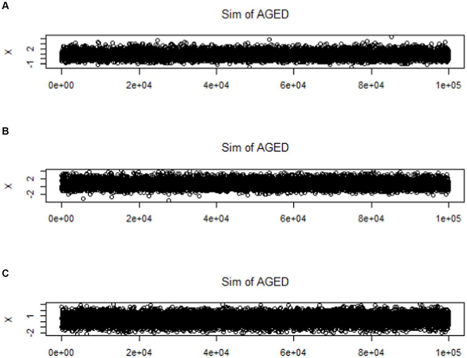
Figure 5. Graphs of realized random samples of size 100,000 taken from AGED with the corresponding pdf (5): (A) design 1, (B) design 2, and (C) design 3.

Figure 6

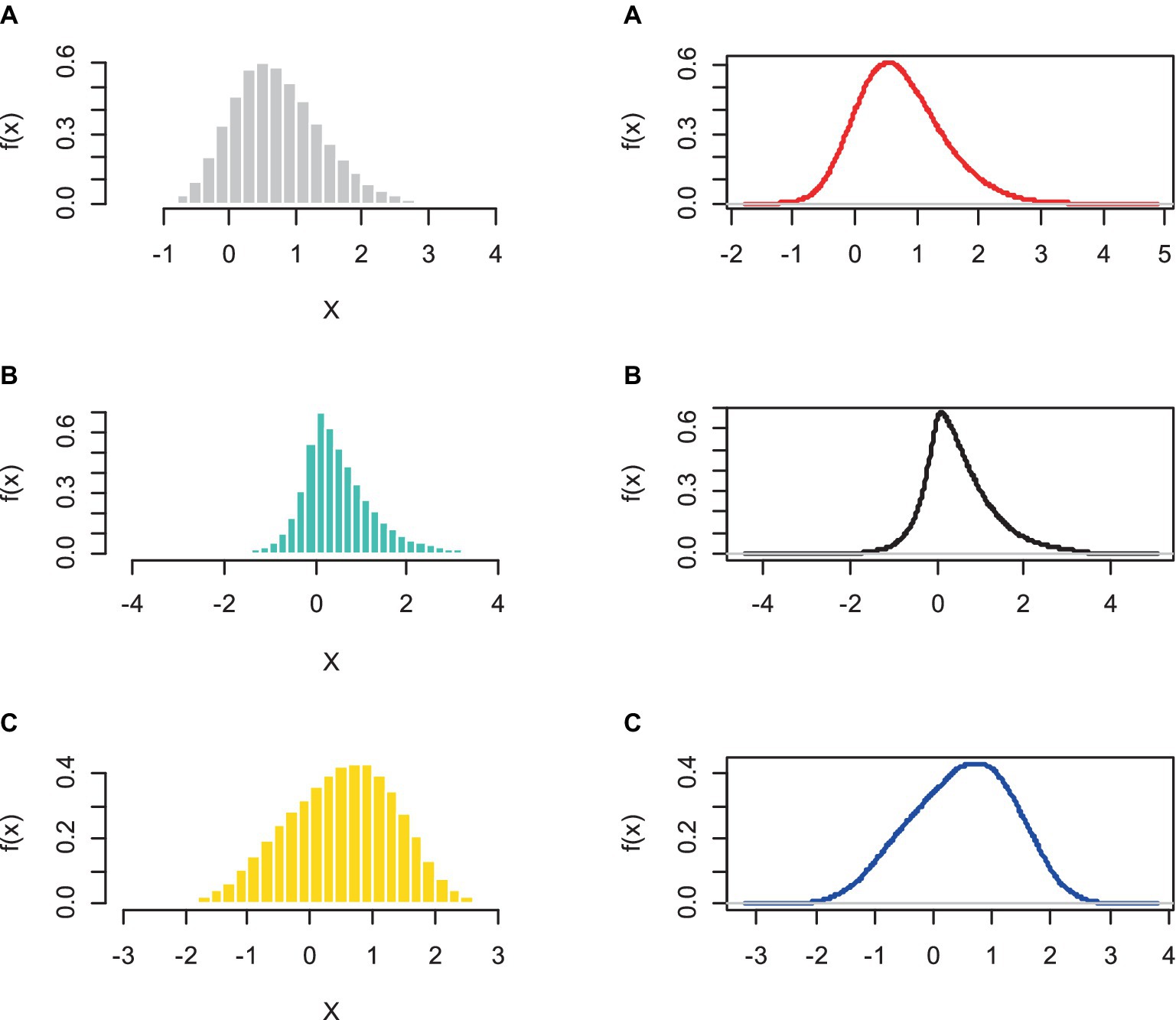
Figure 6. Histograms (left) and density (right) of random samples of size 100,000 taken from AGED with corresponding pdf (5): for (A) design 1, (B) design 2, and (C) design 3, respectively.

The histogram and density of the AGED are plotted. All points under the curve are an accepted random sample and have $x-$ coordinated distributed AGED. The points above the curve are rejected.

8 Parameter estimation using the MLE method

8.1 Applications—fitting to simulated data

In this section, we study and evaluate the long-term performance of the maximum likelihood estimators (MLEs) of AGED parameters based on finite random samples. Several finite samples of sizes $n=100$, 500, 1,000, and 100,000 are considered. Three different designs for parameters $\mu ,\sigma ,\beta ,$ and $\alpha$ are considered. Thus, asymmetry and kurtosis are constructed.

For each sample size $\left(n\right)$ and the specified values of the parameters defined in the simulation design, datasets are generated from the AGED, as per Eq. 5. From each dataset, the estimates of the parameters $\left(\mu ,\sigma ,\beta ,\alpha \right)$ are obtained by the maximum likelihood method. For comparing the performance of the estimators, we use bias and mean square error (MSE) (43).

The average estimates of the parameters, bias, and MSE are calculated using an optimization algorithm in R software. The result verifies the consistency of MLEs. The consistency of MLE can be verified as bias, and the MSE of the estimators is reasonable and diminished for increasing sample size, indicating that estimated values of parameters tend to their true value (Tables 2–4).

Table 2

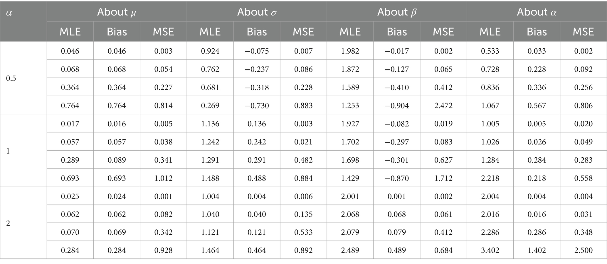
Table 2. Bias and MSE of the maximum likelihood estimators of design 1.

Table 3

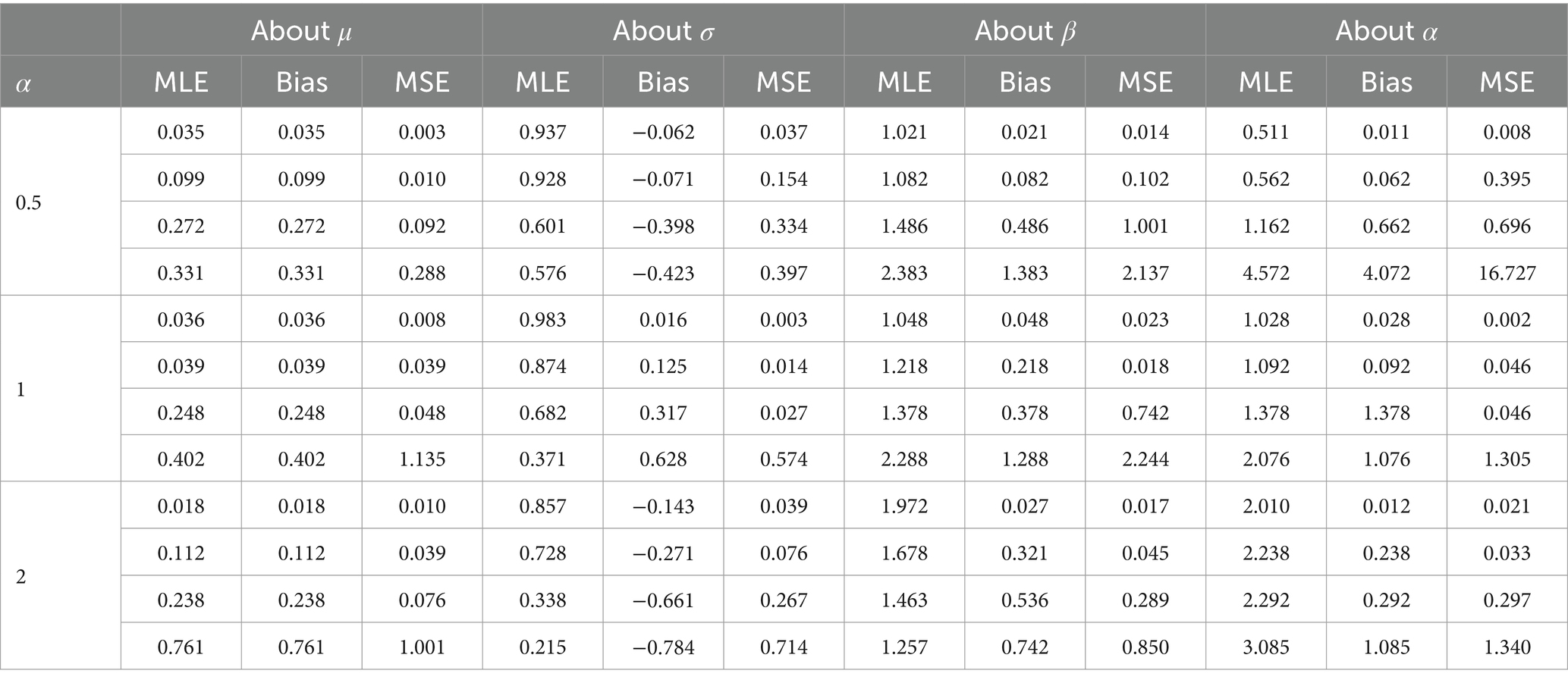
Table 3. Bias and MSE of the maximum likelihood estimator of design 2.

Table 4

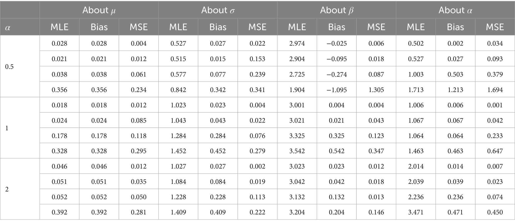
Table 4. Bias and MSE of the maximum likelihood estimator of design 3.

8.2 Applications—fitting to real data

In this section, we illustrate the modeling performance of the asymmetric generalized error distribution (AGED) by modeling data with asymmetry and excess kurtosis. Three practical datasets are used to assess the performance of AGED compared to other distributions.

8.2.1 Datasets

Three practical datasets are considered. The first data are the cyber attacks, which are measured as the average length time of cyber attacks per week. It consists of an average time of attacks of 363 weeks and is obtained from (44).

The second dataset is heart failure data. This dataset comprises a substantial number of individuals diagnosed with heart failure and its associated factors, which consists of 304 patients following treatment and was taken from (45). In this respect, we model a number of cholesterol levels in heart failure patients. Statistical measures and the ML estimates of the AGED are obtained and compared with the competing distributions.

The third dataset is reported in (46), which includes 63 observations of the strengths of 1.5 cm of glass fiber, originally obtained from workers at the National Physical Laboratory, England, and used in the work (47). We have utilized these data to present the modeling performance of the AGED compared to other competing distributions. Table 5 reports the summary of data, whereas the goodness of fit (GOF) statistics can be viewed in Tables 6–8.

Table 5

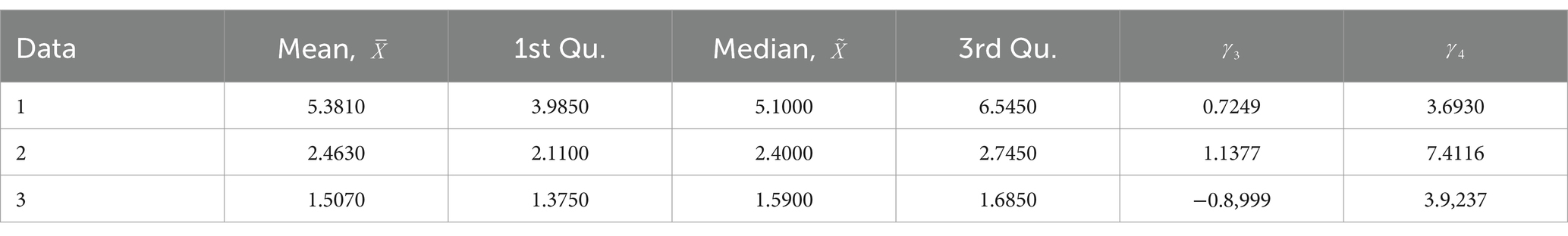
Table 5. Summary statistics of datasets.

Table 6

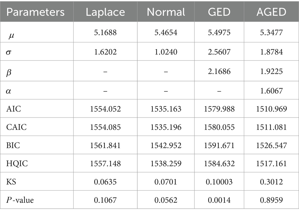
Table 6. MLEs and GOF statistics results of the cyber dataset.

Table 7

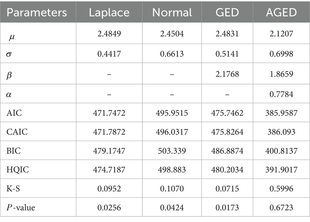
Table 7. MLEs and GOF statistics results of the heart failure dataset.

Table 8

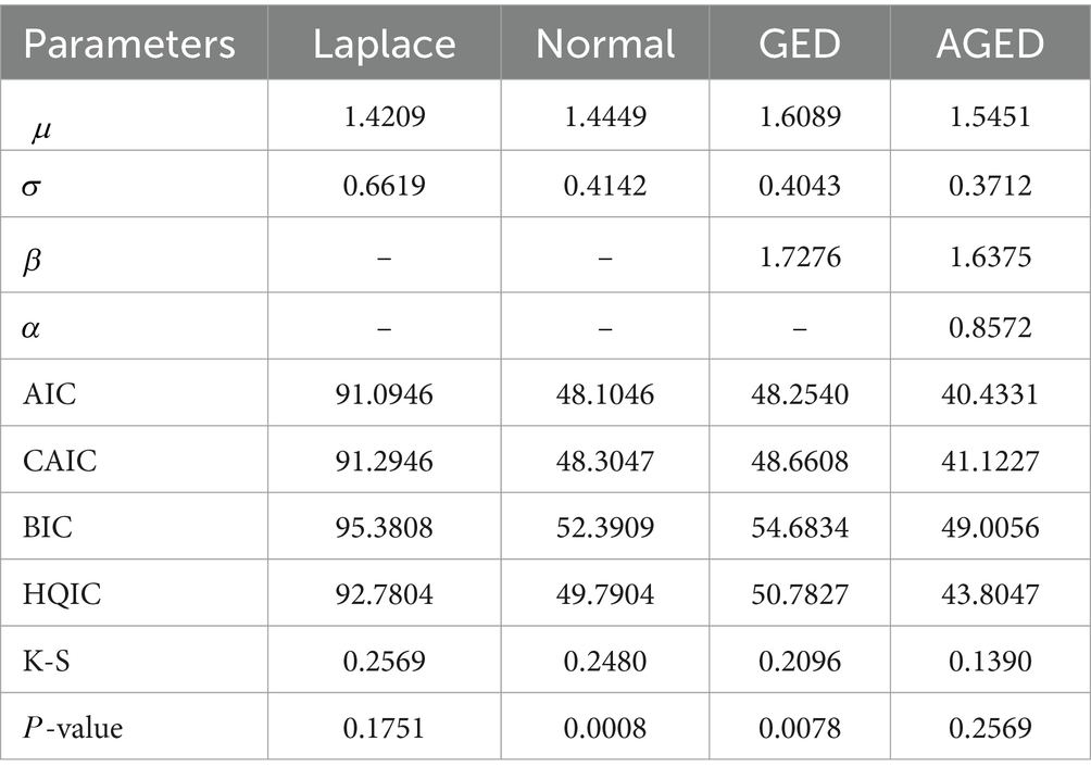
Table 8. MLEs and GOF statistics results of the strengths of glass fibers dataset.

Some descriptive statistics for the data, including skewness and kurtosis coefficients, are displayed in Table 5, where ${\gamma }_3$ and ${\gamma }_4$ denote skewness and kurtosis coefficients, respectively. In this respect, we highlight the peakedness and asymmetry of the data.

Second, different distributions are considered to model these datasets. There are many distributions that have been proposed; however, distributions having special cases for the suggested pdf would be used. The generalized error distribution, the Laplace distribution, and the normal distribution are used to fit the data and are compared with AGED.

We examined the performance of the AGED. Using mostly the prominent goodness-of-fit statistics, Kolmogorov–Smirnov statistics (K-S), consistent Akaike’s information criteria (CAIC), Hannan–Quinn information criteria (HQIC), and Bayesian information criterion (BIC) (48), we compared the competing distribution with AGED.

When the estimates of parameters are computed, we examine via GOF statistics which of the four pdfs is the best fit for the data. The lower those values, the better the fit (48–50). The corresponding maximum likelihood estimates and goodness-of-fit (GOF) statistics are presented in Tables 6–8.

It can be seen that the GOF statistic values of the AGED are lower than those of competing distributions, indicating its superiority in fitting all datasets compared to competing distributions. In light of this, we can conclude that the AGED provides a better fit than a competing distribution.

Figures 7–9 display the histogram of the three practical datasets with the estimated pdf of the AGED along with the competing distributions. The figures show that a closer fit to the data was provided by the AGED for all datasets. In light of this, we can draw the conclusion that the AGED is a better fit for all datasets compared to competing distributions.

Figure 7

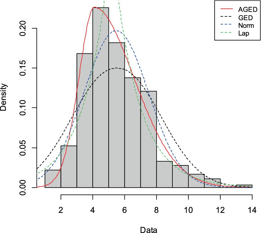
Figure 7. Histogram and fitted probability density function of AGED, GED, Normal, and Laplace distribution for cyber dataset.

Figure 8

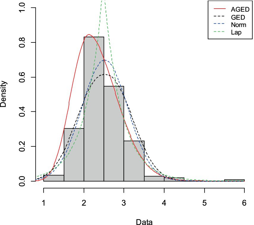
Figure 8. Histogram and fitted probability density function of AGED, GED, Normal, and Laplace distribution for heart failure dataset.

Figure 9

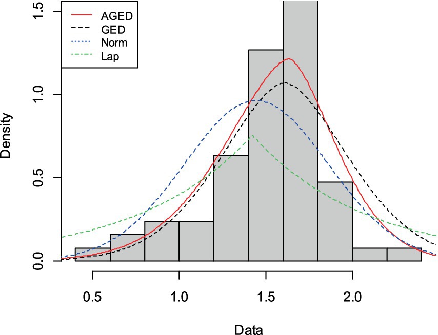
Figure 9. Histogram and fitted probability density function of AGED, GED, Normal, and Laplace distribution for strengths of glass fibers dataset.

For all datasets, Figures 7–9 show that AGED fits better than the competing distributions. In particular, the peakedness can be fitted. The asymmetry illustrated in Table 5 has also been fitted, as unequally distributed histograms around the location in the figures can show that there is an asymmetry in the datasets.

9 Conclusion

The main finding of this study is the derivation of a new probability distribution that reveals interesting properties, especially with various asymmetry and kurtosis behaviors; we call it the asymmetric generalized error distribution (AGED). AGED is a new contribution to the field of statistical theory and provides a more flexible pdf, cdf, and hazard function than the base distribution. The mathematical and statistical features of the distribution are derived and discussed. To estimate the distribution parameters, maximum likelihood estimators are derived. A simulation study is done using the acceptance-rejection algorithm. In the applications, the datasets have high kurtosis and skewness. The criteria indicate that the AGED provides better fits to the datasets. This implies that the new distribution is a good alternative for modeling data with asymmetric and excess kurtosis behavior. We expect that the distribution can be applied to many more real datasets, and the findings of the study can be used as the basis for future research in the field.

Data availability statement

The raw data supporting the conclusions of this article will be made available by the authors, without undue reservation.

Author contributions

TA: Conceptualization, Investigation, Software, Data curation, Formal analysis, Methodology, Visualization, Writing – original draft, Writing – review & editing. AG: Conceptualization, Software, Data curation, Formal analysis, Methodology, Visualization, Writing – original draft, Writing – review & editing.

Funding

The author(s) declare that no financial support was received for the research, authorship, and/or publication of this article.

Acknowledgments

We thank Kotebe University of Education for providing necessary facilities. The authors also gratefully acknowledge the Editor and referees for their insightful comments and constructive suggestions that led to a marked improvement of the article.

Conflict of interest

The authors declare that the research was conducted in the absence of any commercial or financial relationships that could be construed as a potential conflict of interest.

Publisher’s note

All claims expressed in this article are solely those of the authors and do not necessarily represent those of their affiliated organizations, or those of the publisher, the editors and the reviewers. Any product that may be evaluated in this article, or claim that may be made by its manufacturer, is not guaranteed or endorsed by the publisher.

References

1. Cahoy, DO (2015). Some skew-symmetric distributions which include the bimodal ones. Commun Stat Theory Methods 44:554–63. doi: 10.1080/03610926.2012.746986

Crossref Full Text | Google Scholar

2. Arellano-Valle, RB, Gómez, HW, and Quintana, FA (2005). Statistical inference for a general class of asymmetric distributions. J Stat Plan Infer 128:427–43. doi: 10.1016/j.jspi.2003.11.014

PubMed Abstract | Crossref Full Text | Google Scholar

3. Fernández, C, and Steel, MF (1998). On Bayesian modelling of fat tails and skewness. J Am Stat Assoc 93:359–71. doi: 10.1080/01621459.1998.10474117

Crossref Full Text | Google Scholar

4. Abdulah, E, and Elsalloukh, H (2013). Analyzing skewed data with the epsilon skew gamma distribution. J Stat Appl Probab 2:195. doi: 10.12785/jsap/020302

Crossref Full Text | Google Scholar

5. Theodossiou, P (2015). Skewed generalized error distribution of financial assets and option pricing. Multinatl Financ J 19:223–66. doi: 10.17578/19-4-1

Crossref Full Text | Google Scholar

6. Fagiolo, G, Napoletano, M, and Roventini, A (2008). Are output growth-rate distributions fat-tailed? Some evidence from OECD countries. J Appl Econ 23:639–69. doi: 10.1002/jae.1003

Crossref Full Text | Google Scholar

7. Hampel, FR, Ronchetti, EM, Rousseeuw, PJ, and Stahel, WA. (2011). Robust statistics: The approach based on influence functions. New York, USA: John Wiley & Sons.

Google Scholar

8. Arellano-Valle, RB, and Genton, MG (2005). On fundamental skew distributions. J Multivar Anal 96:93–116. doi: 10.1016/j.jmva.2004.10.002

PubMed Abstract | Crossref Full Text | Google Scholar

9. Weldensea, M. (2019). Bayesian analysis of the epsilon skew exponential power distribution. New York, USA: University of Arkansas at Little Rock.

Google Scholar

10. Hutson, AD (2019). An alternative skew exponential power distribution formulation. Commun Stat Theory Methods 48:3005–24. doi: 10.1080/03610926.2018.1473600

PubMed Abstract | Crossref Full Text | Google Scholar

11. Jia, P, Liao, X, and Peng, Z (2015). Asymptotic expansions of the moments of extremes from general error distribution. J Math Anal Appl 422:1131–45. doi: 10.1016/j.jmaa.2014.09.030

Crossref Full Text | Google Scholar

12. Pewsey, A (2000). Problems of inference for Azzalini’s Skewnormal distribution. J Appl Stat 27:859–70. doi: 10.1080/02664760050120542

PubMed Abstract | Crossref Full Text | Google Scholar

13. Azzalini, A, and Valle, AD (1996). The multivariate skew-Normal distribution. Biometrika 83:715–26. doi: 10.1093/biomet/83.4.715

PubMed Abstract | Crossref Full Text | Google Scholar

14. Mudholkar, GS, and Hutson, AD (2000). The epsilon–skew–Normal distribution for analyzing near-Normal data. J Stat Plan Infer 83:291–309. doi: 10.1016/S0378-3758(99)00096-8

Crossref Full Text | Google Scholar

15. Olmos, NM, Varela, H, Gómez, HW, and Bolfarine, H (2012). An extension of the half-Normal distribution. Stat Pap 53:875–86. doi: 10.1007/s00362-011-0391-4

PubMed Abstract | Crossref Full Text | Google Scholar

16. Azzalini, A (1985). A class of distributions which includes the Normal ones. Scand J Stat :171–8. doi: 10.6092/ISSN.1973-2201

Crossref Full Text | Google Scholar

17. Azzalini, A (1986). Further results on a class of distributions which includes the Normal ones. Statistica 46:199–208. doi: 10.6092/issn.1973-2201/711

Crossref Full Text | Google Scholar

18. Ohagan, A, and Leonard, T (1976). Bayes estimation subject to uncertainty about parameter constraints. Biometrika 63:201–3. doi: 10.1093/biomet/63.1.201

PubMed Abstract | Crossref Full Text | Google Scholar

19. Salinas, HS, Arellano-Valle, RB, and Gómez, HW (2007). The extended skew-exponential power distribution and its derivation. Commun Stat Theory Methods 36:1673–89. doi: 10.1080/03610920601126118

Crossref Full Text | Google Scholar

20. Diciccio, TJ, and Monti, AC (2004). Inferential aspects of the skew exponential power distribution. J Am Stat Assoc 99:439–50. doi: 10.1198/016214504000000359

Crossref Full Text | Google Scholar

21. Evans, M, Hastings, N, and Peacock, B (2001). Statistical distributions. Meas Sci Technol 12:117–7. doi: 10.1088/0957-0233/12/1/702

Crossref Full Text | Google Scholar

22. Subbotin, MT (1923). On the law of frequency of error. Математический Сборник 31:296–301.

Google Scholar

23. Tiao, GC, and Box, GE (1973). Some comments on “Bayes” estimators. Am Stat 27:12–4.

Google Scholar

24. Bottazzi, G, and Secchi, A (2011). A new class of asymmetric exponential power densities with applications to economics and finance. Ind Corp Chang 20:991–1030. doi: 10.1093/icc/dtr036

Crossref Full Text | Google Scholar

25. Giller, G. L. (2005). A generalized error distribution. Giller Investments Research. Available at: https://dx.doi.org/10.2139/ssrn.2265027.

Google Scholar

26. Davis, C. (2015). The skewed generalized T distribution tree package vignette. Chicago: R Foundation for Statistical Computing.

Google Scholar

27. Catherine, F, Merran, E, Nicholas, H, and Brian, P. (2011). Statistical distributions. Hoboken: John Wiley & Sons Inc (2011).

Google Scholar

28. Owen, DB (1956). Tables for computing bivariate Normal probabilities. Ann Math Stat 27:1075–90. doi: 10.1214/aoms/1177728074

PubMed Abstract | Crossref Full Text | Google Scholar

29. Young, J, and Minder, CE (1974). Algorithm AS 76: an integral useful in calculating non-central T and bivariate Normal probabilities. Appl Stat :455–7. doi: 10.2307/2347148

Crossref Full Text | Google Scholar

30. Hill, I (1978). A remark on algorithm AS 76: an integral useful in calculating non-central T and bivariate Normal probabilities. J R Stat Soc C Appl Stat 27:379–9. doi: 10.1111/j.1467-9876.1978.tb01084.x

Crossref Full Text | Google Scholar

31. Boys, RJ (1989). Algorithm AS R80: a remark on algorithm AS 76: an integral useful in calculating noncentral T and bivariate Normal probabilities. J R Stat Soc C Appl Stat 38:580–2. doi: 10.2307/2347894

Crossref Full Text | Google Scholar

32. Lehmann, EL. Elements of large-sample theory. (1999). New York, USA: Springer.

Google Scholar

33. Altman, DG. Practical statistics for medical research. (1990). New York, USA: CRC Press.

Google Scholar

34. Astorga, JM, Reyes, J, Santoro, KI, Venegas, O, and Gómez, HW (2020). A reliability model based on the incomplete generalized Integro-exponential function. Mathematics 8:1537. doi: 10.3390/math8091537

PubMed Abstract | Crossref Full Text | Google Scholar

35. Fox, J, Weisberg, S, Adler, D, Bates, D, Baud-Bovy, G, Ellison, S, et al. (2012). Package ‘car’. Vienna: R Found. Statist. Comput. 16:333.

Google Scholar

36. Karr, AF. Introduction to Probabiity. (1999). New York, NY: Springer New York.

Google Scholar

37. Team, RDC. (2010). R: a language and environment for statistical computing. R Foundation for Statistical Computing.

Google Scholar

38. Arellano Valle, R. B., Gómez Geraldo, H., and Salinas, H. S. (2013). A note on the fisher information matrix for the skew-generalized-Normal model. SORT-Statistics and Operations Res. Trans. 37, 19–28.

Google Scholar

39. Lange, K, Chambers, J, and Eddy, W. (2010). Numerical analysis for statisticians, vol. 1 New York: Springer.

Google Scholar

40. Nguyen, N, and Ökten, G (2016). The acceptance-rejection method for low-discrepancy sequences. Monte Carlo Methods Appl 22:133–48. doi: 10.1515/mcma-2016-0104

Crossref Full Text | Google Scholar

41. Casella, G, and Berger, RL. Statistical inference (Cengage Learning). Belmont, CA, USA. 47–218.

Google Scholar

42. Moskowitz, B, and Caflisch, RE (1996). Smoothness and dimension reduction in quasi-Monte Carlo methods. Math Comput Model 23:37–54. doi: 10.1016/0895-7177(96)00038-6

Crossref Full Text | Google Scholar

43. Ahmed, AA, Algamal, ZY, and Albalawi, O (2024). Bias reduction of maximum likelihood estimation in Exponentiated Teissier distribution. Front Appl Math Stat 10:1351651. doi: 10.3389/fams.2024.1351651

Crossref Full Text | Google Scholar

44. Kaggle. (2023). Heart Failure Datasets. Available at: https://www.kaggle.com/Datasets/Vaibhavsuman/Heart-Failure-Dataset

Google Scholar

45. Gjika, E. Fitting probability distribution in R. Dataset Cyber Data (2021). Available at: https://rpubs.com/Eraldagjika/715261.

Google Scholar

46. Smith, RL, and Naylor, J (1987). A comparison of maximum likelihood and Bayesian estimators for the three-parameter Weibull distribution. J R Stat Soc C Appl Stat 36:358–69. doi: 10.2307/2347795

Crossref Full Text | Google Scholar

47. Baharith, LA, and Aljuhani, WH (2021). New method for generating new families of distributions. Symmetry 13:726. doi: 10.3390/sym13040726

PubMed Abstract | Crossref Full Text | Google Scholar

48. Akaike, H (1974). A new look at the statistical model identification. IEEE Trans Autom Control 19:716–23. doi: 10.1109/TAC.1974.1100705

Crossref Full Text | Google Scholar

49. Schwarz, G (1978). Estimating the dimension of a model. Ann Stat. 6:461–4.

Google Scholar

50. Algamal, ZY, Alobaidi, NN, Hamad, AA, Alanaz, MM, and Mustafa, MY (2024). Neutrosophic Beta-Lindley distribution: mathematical properties and modeling bladder Cancer data. Int J Neutrosophic Sci 23:186–6. doi: 10.54216/IJNS.230215

Crossref Full Text | Google Scholar