 Roman Taranets
 Nataliya Vasylyeva
 Belgacem Al-Azem
- 1Department of Nonlinear Analysis and Equations of Mathematical Physics, Institute of Applied Mathematics and Mechanics of National Academy of Sciences of Ukraine, Slovyansk, Ukraine
- 2Department of Hydrodynamics of Wave and Channel Processes, Institute of Hydromechanics of National Academy of Sciences of Ukraine, Kyiv, Ukraine
- 3Dipartimento di Matematica, Politecnico di Milano, Milan, Italy
- 4Institute of Mathematical Sciences, Claremont Graduate University, Claremont, CA, United States
Compartmental models are widely used in mathematical epidemiology to describe the dynamics of infectious diseases or in mathematical models of population genetics. In this study, we study a time-dependent Susceptible-Infectious-Susceptible (SIS) Partial Differential Equation (PDE) model that is based on a diffusion-drift approximation of a probability density from a well-known discrete-time Markov chain model. This SIS-PDE model is conservative due to the degeneracy of the diffusion term at the origin. The main results of this article are the qualitative behavior of weak solutions, the dependence of the local asymptotic property of these solutions on initial data, and the existence of Dirac delta function type solutions. Moreover, we study the long-term behavior of solutions and confirm our analysis with numerical computations.
1 Introduction
Despite undeniable, vast modern improvements in the development of highly efficient antibiotics and vaccines, infectious diseases still contribute significantly to deaths worldwide. The earlier recognized diseases such as cholera or plague still sometimes pose problems in underdeveloped countries, even erupting occasionally in epidemics. In developed countries, new diseases are emerging, such as the case of AIDS (1981) or hepatitis C and E (1989–1990). New variants are constantly surfacing, such as recent bird flu (SARS) epidemic in Asia, the very dangerous Ebola virus in Africa, and the recent worldwide spread of COVID-19. Overall, infectious diseases continue to be one of the most significant and challenging health problems.
Modeling of epidemiological phenomena has a very long history. The first model for smallpox was formulated by Daniel Bernoulli in 1760. A large number of models have been constructed and analyzed from the early 20th century in response to epidemics of various infectious diseases [see for example [1–6] (and references therein)]. Compartmental models are well established as mathematical modeling techniques. It is often applied to the mathematical modeling of infectious diseases. In this type of modeling, the population is subdivided into compartments or categories such as susceptible, infectious, and recovered in the widely used SIR model or susceptible, infectious, and susceptible like in SIS epidemiological scheme. Here, we are interested in analyzing the SIS model that provides the simplest description of the dynamics of a disease that is contact-transmitted and that does not lead to immunity like it is the case for COVID-19. Discrete-time Markov chain-type SIS models are considered to be a classical approach in modern mathematical modeling in epidemiology. The most recent development in mathematical epidemiology is based on the introduction of continuous modeling based on partial differential equations like in [7, 8].
In our study, for T>0 and Ω = (0, 1), ΩT = Ω × (0, T), we study a time-dependent Susceptible-Infectious-Susceptible (SIS) model derived in the study mentioned in the reference [9], which is a generalized PDE version of a Kimura model [see [10]] in the unknown function p: = p(x, t): :
coupled with the boundary condition
and initial data
Here, represents the fraction of infected, N is the size of the population of interest, p is the probability to find a fraction x at time t in a population of size N, and R0≥0 is the basic reproductive factor.
are connected with variance and the mean of the change of x in the frame of Kimura model. Note that (1.1) is parabolic equation with non-negative characteristic form, and it is degenerated on the boundary of the domain at x = 0. The corresponding Fichera function for (1.1) [see e. g. [11, (1.1.3), p.17]] is on {x = 0} × {t>0}. Hence, according to [11, 12], the problem (1.1–1.3) is well-posed without any boundary conditions at x = 0 for all t>0. Reduced number of boundary conditions required for well-posedness of degenerated problems is a well-known phenomenon, and some interesting examples are shown in the study mentioned in the reference [13, 14]. Imposing zero boundary condition at x = 0 makes the problem to be over-determined, and because some weak solutions have this property, the set of solutions for the over-determined problem will not be empty.
It is worth noting that processes defined by similar models were studied by Feller in the early 1950s and used to great effect by Kimura, et al. in the 1960s and 70s to give quantitative answers to a wide range of questions in population genetics. However, rigorous analysis of the analytic properties of these equations is only the focus of applied mathematicians. The study of initial or/and initial-boundary value problems for degenerated equations, including Kimura-type operators, has a long history. Here, we do not provide a complete survey of the published results pertaining to these degenerated equations. Instead, we survey some of them for the benefit of the interested reader. Indeed, the investigation of elliptic and parabolic problems, leading to degenerated equations containing operators such as
with a(x) ≈ |x|α, α > 0, and aij and satisfying ellipticity conditions, are extensively studied by many authors with various analytical approaches [see e.g. [11, 12, 15–26]] including stochastic calculus [27–35].
Under suitable assumptions on the asymptotic behavior of the operator's coefficients at the boundary of the domain, the uniqueness of bounded and unbounded solutions, as well as solutions belonging to the weighted Sobolev spaces, was shown in the study mentioned in the reference [12, 20, 22–24, 36] without prescribing any boundary conditions at the origin. The qualitative properties of the corresponding solutions, including the maximum principle and the Harnack inequality, are discussed in the study mentioned in the reference [31–33, 37–39] (see also references therein). Local asymptotic behavior of solutions for different types of degenerate equations was rigorously studied in the study mentioned in the reference [40–42]. We also refer the reader to the study mentioned in the reference [30–32, 34, 43], where the theories of existence and uniqueness of solutions to stochastic differential equations with degenerate diffusion coefficients are developed. Additionally, the well-posedness of the related problems in the case of α = 1 is discussed in the study mentioned in the reference [27–29]. It is worth noting that degenerate diffusion is examined in the context of measure-valued process [see [44–46]] via the semigroup techniques [47–49].
Finally, for the well-posedness of parabolic degenerate problems, we refer to the study mentioned in the reference [15, 16, 18, 21, 25, 26, 35, 50–52], where the existence of weak and classical solutions is established for different values of α>0. Previous researchers such as Chen and Weth-Wadman [53] and Epstein and Mazzeo [31] restricted their attention to the solutions with the best possible regularity properties, which leads to considerable simplifications and limitations. For real applications, it is important to consider solutions with more complicated behavior, which is the goal of our study.
The outline of the study is as follows: in Section 2, we show the existence of stationary solutions, analyze the dependence of their asymptotic behavior, near the origin, on initial data, confirm numerically their meta-stability, and analyze convergence; in Section 3, we analyze particular classical and weak solutions. We used COMSOL Multiphysics® software to perform the numerical simulations [54].
2 Weak solutions: convergence to steady state and asymptotic behavior as t → +∞
Throughout the whole article, we encounter the usual spaces W1, p(Ω), Lp(Ω), and . It is worth noting that the last class is a weighted space L2 with a weight ω and the induced norm
Moreover, we use the notations H1(Ω) and for W1, 2(Ω) and , respectively.
In this section, as it is mentioned in the introduction, we discuss the long-term behavior of a weak solution to problem (1.1–1.3). To that end, we first construct the explicit stationary solution Ps: = Ps(x): related to (1.1-1.3), and then, we examine a set of initial data which provide the convergence of the weak solution as T → +∞. In particular, we consider a case of convergent p(x, t) to Ps(x).
2.1 Existence of a steady state
First, we start with getting an analytical formula for a stationary solution for (1.1):
coupled with the boundary condition:
Integrating (2.1) in x and taking into account (2.2), we get
It is apparent that this equation has a general solution
where
As a result, we obtain the explicit form of the classical stationary solution to (1.1–1.3)
Observe that the changing-sign convection term for R0 = 2 equals zero at x = 0.5, leading to a wave-like solution that moves toward this point, forming a meta-stable steady-state shape. This illustrates that the solution's short-term behavior is driven by the convection, as shown in Figures 1, 2. It takes a long-time for meta-stable steady state (a wave-like solution that slowly changes its shape) to move mass toward the origin. These long-term dynamics are due to a slow diffusion effect, and eventually, the solution blows up at the origin, which is indeed the case for two different sets of parameter values, as shown in Figures 3, 4. All numerical simulations show high accuracy of the mass conservation property even for long-term computations, which suggests the existence of a solution of Delta function type that acts as a global attractor in this dynamical system.

Figure 1. These two pictures illustrate the dominant behavior of convection in the short-term t ∈ [0, 0.1]. (Left) Convection moves the solutions toward the steady state from the right side to the left one for R0 = 2 and N = 200, (Right) convection moves the solutions toward the steady state from the left side to the right one for the same parameter values. The initial data are plotted with a dashed line.
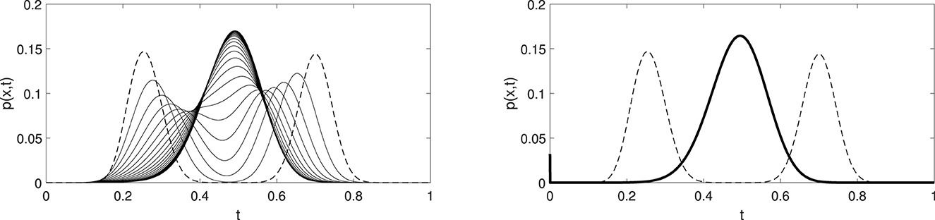
Figure 2. These two pictures illustrate t ∈ [0, 0.1] short-term dynamics for R0 = 2 and N = 100 (Left) and t ∈ [0, 2000] long-term dynamics with blow up at the origin (Right). The initial data are plotted with a dashed line.
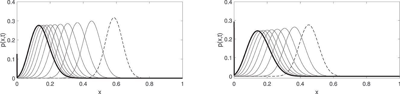
Figure 3. These two pictures illustrate the dominant behavior of convection in the short-term t ∈ [0, 0.1]. (Left) Convection moves solutions toward the origin, here R0 = 0.5 and N = 100 and where solutions blow up. (Right) Convection again moves solutions toward the origin, here R0 = 1 and N = 100 and where solutions blow up. The initial data are plotted with a dashed line.
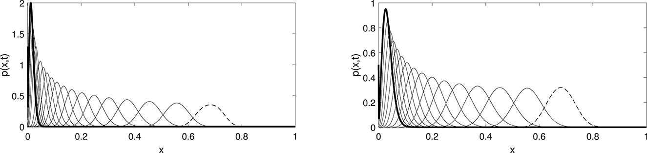
Figure 4. These two pictures illustrate the dominant behavior of convection in the short term t ∈ [0, 0.1]. (Left) Convection moves solutions toward the origin, here R0 = 0 and N = 100, where the solutions blow up. (Right) Convection again moves solutions toward the origin, here R0 = 0 and N = 200, where the solutions blow up. The initial data are plotted with a dashed line.
2.2 Long-term behavior of a weak solution
Assuming that ω(x) is defined by Equation (2.4) and that
We define a weak solution of (1.1–1.3) in the following sense:
Definition 2.1. A non-negative function is a weak solution of problem (1.1)–(1.3) for any T>0 if
and p satisfies (1.1) in the sense
for all ψ ∈ L2(0, T; H1(Ω)), and ψ (0, t) = 0 for allt ∈ [0, T]. Here, is a dual pair of elements u ∈ (H1)′ and v ∈ H1.
Now, we are ready to state our first main result related to the asymptotic behavior of a weak solution to (1.1–1.3).
Theorem 1. (i) Let and , a weak solution p(x, t) satisfies the relation
Moreover, if , ω(x)p(x, t)∈C([0, +∞);H1(Ω)), and there is convergence
(ii) Let , if p(x, t) is a weak solution to (1.1–1.3) and , where is the same constant as in Equation (2.3), there exists a constant , depending on R0 and N, such that
Moreover, if , there exist a constant C1>0 and a time T*>0, depending on R0 and N, such that
Numerical simulations in Figures 5, 6 illustrate the convergence result in Equation (2.6).
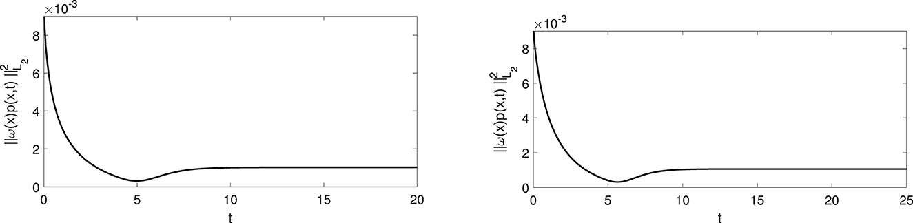
Figure 5. These two pictures illustrate convergence of weighted L2-norm of p(x, t) to a constant for R0 = 0 and N = 100, (left) and R0 = 0 and N = 200, (right).
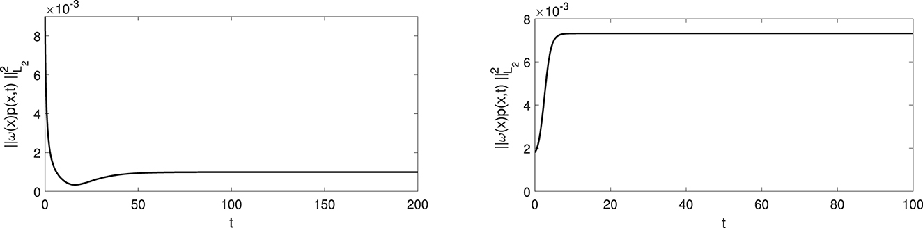
Figure 6. These two pictures illustrate convergence of weighted L2-norm of p(x, t) for R0 = 0.5 and N = 100, (left) and R0 = 2 and N = 200, (right).
Note that Theorem 1 describes a behavior of a weak solution to direct well-posed problem (1.1)–(1.3), depending on the different types of behavior ω(x)p(x, t) at x = 0, taking into account two explicit solutions: steady state (subsection 2.1) and Fourier series solutions (subsection 3.1). In other words, our main result has a conditional characteristic via inserting additional assumptions on the term ω(x)p(x, t) as x → 0 in the statement of the Theorem 1 but not to the statement of the problem (1.1)–(1.3). In the context of infectious disease spreading dynamic, Theorem 1 says that a different regularity of the initial data at x = 0 leads to a different rate of the disease extinction, i. e., more regular initial data give us faster decay of infection.
Remark 2.1. In this study, we do not discuss the existence and uniqueness of weak solutions vanishing at the origin. As for these issues, we refer the interested readers to Section 7 in the study mentione4d in the reference [51], where the related questions are analyzed.
Remark 2.2. In particular, Theorem 1 provides the following properties:
(i) (2.5) implies
where we deduce that limt → +∞p(x, t) = 0 a. e. ;
(ii) (2.6) gives the stability of the steady state Ps.
Proof of Theorem 1. Introducing a new function z: = ω(x)p(x, t) and rewriting problem (1.1)–(1.3) in the more suitable form:
Note that if , we can define a new function , and we reduce the case to a problem similar to Equation (2.7). Since the approximation approach is well developed for this type of problem, to avoid technical details, we proceed with formal computations. Our formal computations can be rigorously justified by introducing a sequence of approximate solutions with extra regularity property, taking advantage of the standard approximation arguments, and passing to the limit in the final estimates. The weak solution will be obtained as a limit as ε → 0 of smooth solutions for the corresponding approximating problems. For any ε>0, we consider the approximating problems of Equation (2.7), where instead of ω(x) and z0(x), we take and such that zε, 0(x) → z0(x) strongly in H1(Ω) as ε → 0. As these approximating problems are uniformly parabolic, by general PDE theory for the second order parabolic equations (see, e.g. [55]), we find a solution . By going through all routine calculations for zε, and then passing to the limit with respect to ε → 0, we arrive at the required estimates for the corresponding limit solution z.
We now verify claim (i) of Theorem 1. To this end, multiplying the equation in (2.7) by z(x, t) and integrating over Ω, we obtain as follows:
Next, we take advantage of Hardy inequality [56, p. 22, (1.25) with p = q = 2]
with z(0) = 0. Here, the constant CH(R0) satisfies the inequalities:
Note that
where it follows that . Thus, statement (2.8) along with Hardy inequality, see [9], leads to the relation
Multiplying the equation in (2.7) by and integrating over Ω, we obtain the equation
which implies
To handle the second term in the left-hand side of this equality, we apply to the following inequality:
Hence, we end up with the relation
As a result, we obtain the following convergence:
provided the following inequality holds:
As a simple consequence of this fact and the convergence of (2.9), we obtain an upper bound on z(x, t):
which, in turn, provides the desired relation
We now proceed by showing that statement (ii) of Theorem 1 is in fact valid. We multiply (2.7) by ω(x)ψ(x)z(x, t) and integrate over Ω to obtain
Then, choosing here
we arrive at the equality
where
Thus, we easily conclude that
where Now, multiplying the equation in (2.7) by and integrating over Ω, we obtain
Now, consider ϕ(x) such that (ω(x)ϕ′(x))′F2(x) = 2f(x)ψ(x), i. e.,
we have
The above equality, along with (2.10), leads to
Now, applying to , the following estimate
where
to (2.11) and conclude that
where
As a result, there exists a time T*>0 such that
provided the following inequality holds:
This completes the proof of assertion (ii) and, as a consequence, of Theorem 1.
3 Solutions in weighted L2-space
In this section, we will illustrate an application of Theorem 1 by constructing solutions, using the spectral decomposition method, in a weighted L2-space. First, we analyze classical solutions to problem (2.7), and then, we discuss some classes of weak solutions.
3.1 Fourier series solutions in a weighted space
Introducing a new variable
and denoting by
we rewrite problem (2.7) in the form as follows:
It is worth noting that to establish (3.1), we have made use of the following simple and verifiable relations:
or as consequence
Separating variables in (3.1):
leads to the problems
where
with
Now, multiplying (3.2) by , we immediately obtain the equation
Then, setting
we arrive at the classical Sturm–Liouville problem with the continuous potential q(s)
From here, we rely on standard computational methods to obtain the following asymptotic behavior of eigenvalues and eigenfunctions to problem 3.3:
or returning to (3.2):
Thus, problem (3.1) has a particular solution
which, in turn, means
where
Finally, keeping in mind the relation z(x, t) = ω(x)p(x, t), we deduce the formal solution
that is a weak solution in a weighted L2-space in the sense of the Definition 2.1. It is worth noting that the asymptotic behavior of the solution as x → 0+ is in agreement with Theorem 1 (i).
3.2 The Dirac delta function solutions
In this section, we show that Dirac delta function type solutions belong to our class of weak solutions. The main problem here is that, with zero on the boundary, the integral is a priori not well defined (over-determined ill-posed problem was previously considered in the study mentioned in the reference [9]). Now, we denote positive and non-negative cut of functions by f(x)χ{x>0} and f(x)χ{x≥0}, respectively. This corresponds to integrating δ function against the function f(x)χ{x>0} (or possibly f(x)χ{x≥0}), which is not continuous at the origin x = 0, where the support of the Dirac delta function lies. With the Dirac delta function at the boundary of the integration, only formal expressions could be found in the literature: . This is the justification for choosing a symmetrization method by considering a problem of extended domain [−1, 1] for our Dirac delta function type solutions. Now, we look for a solution to a symmetrically extended problem (1.1)–(1.3) on the interval (−1, 1) in the form of p(x, t) = η(t)δ0(x), where δ0(x) is the Dirac delta function concentrated at the origin.
Multiplying symmetrized Equation (1.1) by ϕ(x)∈C2[−1, 1] with compact support and ϕ(0)≠0, after integrating by parts in QT: = (−1, 1) × (0, T), we have
where and are even continuation of f and g, respectively. Taking p(x, t) = η(t)δ0(x) in the last equality, we deduce that
Due to the inequality ϕ(0)≠0, we have
As a result, symmetrized Equation (1.1) has the following solution:
Convergence of a weak solution to the Dirac delta function is shown in Figure 7. It is interesting to mention that a non-smooth change of variables (for the case R0 = 0) will remove the degeneracy from the equation. However, the whole long-term dynamics will not be recovered in terms of y as a global attractor-type solution. Cet that satisfies no-flux boundary conditions in terms of variable y will not be satisfying no-flux boundary conditions in terms of variable x. Although Cet solves the original problem with Neumann boundary conditions (which make the original problem ill-posed), it is unstable. Indeed, a slight perturbation will drive the dynamics toward the Dirac delta function.
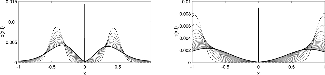
Figure 7. These two pictures illustrate the existence of the Dirac delta function type solutions for symmetrized problems with R0 = 0 and N = 10. The initial data are plotted with a dashed line.
Data availability statement
The original contributions presented in the study are included in the article/supplementary material, further inquiries can be directed to the corresponding author.
Author contributions
RT: Writing – original draft. NV: Writing – original draft. BA-A: Writing – original draft.
Funding
The author(s) declare financial support was received for the research, authorship, and/or publication of this article. RT and NV were partially supported by the Foundation of the European Federation of Academy of Sciences and Humanities (ALLEA), the Grant EFDS-FL2-08.
Conflict of interest
The authors declare that the research was conducted in the absence of any commercial or financial relationships that could be construed as a potential conflict of interest.
Publisher's note
All claims expressed in this article are solely those of the authors and do not necessarily represent those of their affiliated organizations, or those of the publisher, the editors and the reviewers. Any product that may be evaluated in this article, or claim that may be made by its manufacturer, is not guaranteed or endorsed by the publisher.
References
1. Allen LJS. Some discrete-time SI, SIR, and SIS epidemic models. Mathemat Biosci. (1994) 124:83–105. doi: 10.1016/0025-5564(94)90025-6
2. Allen LJS, Burgin AM. Comparison of deterministic and stochastic SIS and SIR models in discrete time. Math Biosci. (2000) 163:1–33. doi: 10.1016/S0025-5564(99)00047-4
3. Bailey NTJ. The mathematical Theory of Infectious Diseases and its Applications, 2nd Edition. New York: Hafner Press [Macmillan Publishing Co., Inc.] (1975).
4. Diekmann O, Heesterbeek H, Britton T. Mathematical Tools for Understanding Infectious Disease Dynamics. Princeton, NJ: Princeton University Press (2013).
6. Feng Z, Huang W. Castillo-Chavez C. Global behavior of a multi- group sis epidemic model with age structure. J Differential Equat. (2005) 218:292–324. doi: 10.1016/j.jde.2004.10.009
7. Wang Y, Xu K, Kang Y, Wang H, Wang F, Avram A. Regional influenza prediction with sampling twitter data and pde model. Int J Environ Res Public Health. (2020) 17:678. doi: 10.3390/ijerph17030678
8. Li XZ, Yang J, Martcheva M. Age Structured Epidemic Modeling. Vol. 52. Cham: Springer Nature (2020).
9. Chalub ACC, Souza MO. Discrete and continuous SIS epidemic models: a unifying approach. Ecol Compl. (2014) 18:83–95. doi: 10.1016/j.ecocom.2014.01.006
10. Kimura M. On the probability of fixation of mutant genes in a population. Genetics. (1962) 6:713. doi: 10.1093/genetics/47.6.713
11. Oleinik OA, Radkevic EV. Second-Order Equations with Non-Negative Characteristic form, 1st Edition. Boston: Springer-Verlag US. (1973).
12. Fichera G. Sulle equazioni differenziali lineri ellittico-paraboliche del secondo ordine. Atti Accad Naz Lincei Mem Cl Sei Fiz Mat Nat Sez I. (1956) 5:1–30.
13. Chugunova M, Karabash IM, Pyatkov SG. On the nature of ill-posedness of the forward-backward heat equation. Integral Equ Operat Theory. (2009) 65:319–44. doi: 10.1007/s00020-009-1720-z
14. Chugunova M, Pelinovsky D. Spectrum of a non-self-adjoint operator associated with the periodic heat equation. J Math Analysis Appl. (2008) 342:970–88. doi: 10.1016/j.jmaa.2007.12.036
15. Bazaliy BV, Krasnoschek NV. Regularity of solutions to multidimensional free boundary problems for the porous medium equation. Math Trudy. (2002) 5:38-91. Available online at: http://mathscinet.ams.org/mathscinet-getitem?mr=1944066
16. Feehan PMN, Pop CA. A Schauder approach to degenerate-parabolic partial differential equations with unbound coefficients. J Differential Equat. (2013) 254:4401–45. doi: 10.1016/j.jde.2013.03.006
17. Feehan PMN, Pop CA. On the martingale problem for degenerate-parabolic partial differential operators with unbounded coefficients and a mimicking theorem for Ito processes. Trans Amer Math Soc. (2015) 367:7565–93. doi: 10.1090/tran/6243
18. Feehan PMN, Pop CA. Boundary-degenerate elliptic operators and Hölder continuity for solutions to variational equations and inequalities. Ann Inst H Poincaré-Anal Nonlin. (2017) 34:1075–129. doi: 10.1016/j.anihpc.2016.07.005
19. Monticelli DD, Punzo F. Distance from sub-manifolds with boundary and applications to Poincaré inequalities and to elliptic and parabolic problems. J Differential Equat. (2019) 267:4274–92. doi: 10.1016/j.jde.2019.04.038
20. Nobili C, Punzo F. Uniqueness for degenerate parabolic equations in weighted L1 spaces. J Evol Equa. (2022) 22:7. doi: 10.1007/s00028-022-00805-7
21. Pozio MA, Punzo F. Tesei A. Criteria for well-posedness of degenerate elliptic and parabolic problems. J Math Pures Appl. (2008) 90:353–86. doi: 10.1016/j.matpur.2008.06.001
22. Pozio MA, Punzo F, Tesei A. Uniqueness and non-uniqueness of solutions to parabolic problems with singular coefficients. DCDS-A. (2011) 30:891–916. doi: 10.3934/dcds.2011.30.891
23. Pozio MA, Tesei A. On the uniqueness of bounded solutions to singular parabolic problems, DCDS-A. (2005) 13:117–37. doi: 10.3934/dcds.2005.13.117
24. Punzo F. Uniqueness of solutions to degenerate parabolic and elliptic equations in weighted Lebesgue spaces. Math Nachr. (2013) 286:1043–54. doi: 10.1002/mana.201200040
25. Stroock D, Varadhan SRS. On degenerate elliptic-parabolic operators of second order and their associate diffusion. Commun Pure Appl Math. (1972) 25:651–713. doi: 10.1002/cpa.3160250603
26. Venni A. Maximal regularity for a singular parabolic problem. Rend Sem Mat Univ Politec Torino. (1994) 52:87–101.
27. Athreya S, Barlow M, Bass R, Perkins E. Degenerate stochastic differential equations and super-markov chains. Probab Theory Related Fields. (2002) 128:484–520. doi: 10.1007/s004400100191
28. Bass RE. Perkins Degenerate stochastic differential equations with HI' older continuous coefficients and super-markov chains. Trunsactions Amer Math Society. (2002) 355:373–405. doi: 10.1090/S0002-9947-02-03120-3
29. Cherny AS. On the uniqueness in law and the path-wise uniqueness for stochastic differential equations. Theory Prob Appl. (2001) 46:483–97. doi: 10.1137/S0040585X97979093
30. Cherny AS, Engelbert H-J. Singular Stochastic Differential Equations. Cham: Springer, Lecture Notes in Mathematics Series. (2005).
31. Epstein CL, Mazzeo R. Degenerate Diffusion Operators Arising in Population Biology, v 185 in the series Annals of Mathematics Studies. Princeton: Princeton University Press. (2013). p. 320.
32. Epstein CL, Mazzeo R. The geometric micro-local analysis of generalized Kimura and Heston diffusion. In: Analysis Topology in Nonlinear Differential Equations Progress and Their Applications. Cham: Springer International Publishing; Birkhäuser (2014). p. 241–266.
33. Epstein CL, Pop CA. Transition probabilities for degenerate diffusion arising in population genetics. Prob Theory Related Fields. (2019) 173:537–603. doi: 10.1007/s00440-018-0840-2
34. Kumar KS. A class of degenerate stochastic differential equations with non-Lipshits coefficients. Proc Indian Acad Sci. (2013) 123:443–54. doi: 10.1007/s12044-013-0141-8
35. Pop CA. Existence, uniqueness and the strong Markov property of solutions to Kimura diffusion with singular drift. Trans Amer Math Soc. (2017) 369:5543–79. doi: 10.1090/tran/6853
36. Punzo F. Integral conditions for uniqueness of solutions to degenerate parabolic equations. J Diff Equa. (2019) 267:6555–73. doi: 10.1016/j.jde.2019.07.003
37. Aronson DG, Besala P. Uniqueness of solutions of the Cauchy problem for parabolic equations. J Math Anal Appl. (1966) 13:516–26. doi: 10.1016/0022-247X(66)90046-1
38. Epstein CL, Mazzeo R. Harnack inequalities and heat-kernel estimates for degenerate diffusion operators arising in population biology. Appl Math Res eXpress. (2016) 2016:217–80. doi: 10.1093/amrx/abw002
39. Epstein CL, Pop CA. The Feynman-kac formula and Harnack inequality for degenerate diffusion. Annuals Probabil. (2017) 45:3336–84. doi: 10.1214/16-AOP1138
40. Vespri V. Analytic semigroups, degenerate elliptic operators and applications to nonlinear Cauchy problems. Annali di Matematica Pura ed Applicata. (1989) 155:353–88 doi: 10.1007/BF01765950
41. Porzio MM, Vespri V. Hölder estimates for local solutions of some doubly nonlinear degenerate parabolic equations. J Differ Equ. (1993) 103:146–78 doi: 10.1006/jdeq.1993.1045
42. DiBenedetto E, Urbano JM, Vespri V. Current issues on singular and degenerate evolution equations. In: Handbook of Differential Equations: Evolutionary Equations 1. North-Holland: Elsevier (2002). p. 169–286.
43. Ethier SN. A class of degenerate diffusion processes occurring in population genetics. Commun Pure Appl Math. (1976) 29:483–93. doi: 10.1002/cpa.3160290503
44. Cerrai S., Clément P. Well-posedness of the martingale problem for some degenerate diffusion processes occurring in dynamics of populations. Bul Sci Math. (2004) 128:355–89. doi: 10.1016/j.bulsci.2004.03.004
45. Dawson DA, March P. Resolvent estimates for Fleming-Viot operators and uniqueness of solutions to related martingale problems. J Func Anal. (1995) 132:417–74. doi: 10.1006/jfan.1995.1111
46. Perkins E. Dawson-watanable super-processes and measure-valued diffusion. In: Lecture Notes in Mathematics. Berlin: Spring-Velag (2001).
47. Barbu V, Favini A, Romanelli S. Degenerate evolution equations and regularity of their associated semigroups. Funkcialaj Ekvacioj. (1996) 39:421-448.
48. Goldstein JA, Cin CY. Degenerate parabolic problems and wentzel boundary condition, semigroup theory applications. Lecture Notes Pure Appl Math. (1989) 116:189–99.
49. Pop CA. C0− estimates and smoothness of solutions to the parabolic equation defined by Kimura operators. J Functional Anal. (2017) 272:47–82. doi: 10.1016/j.jfa.2016.10.014
50. Bazaliy BV, Degtyarev SP. On a boundary-value problem for a strongly degenerate second-order elliptic equation in an angular domain. Ukrain Math J. (2007) 59:955–75. doi: 10.1007/s11253-007-0062-8
51. Chugunova M, Taranets R, Vasylyeva N. Initial-boundary value problems for conservative Kimura-type equations solvability asymptotic and conservation law. J Evol Equ. (2023) 23:17. doi: 10.1007/s00028-023-00869-z
52. Degtyarev SP. Solvability of the first initial-boundary value problem to degenerate parabolic equations in the domains with a singular boundary. Ukr Math Bull. (2008) 5:59–82. Available online at: http://dspace.nbuv.gov.ua/handle/123456789/124297
53. Chen L, Weth-Wadman I. Fundamental solution to 1D degenerate diffusion equation, with locally bounded coefficients. J Math Anal and Appl. (2022) 510:125979. doi: 10.1016/j.jmaa.2021.125979
54. COMSOL Multiphysics. COMSOL AB. COMSOL Multiphysics® v. 6.2. Stockholm (2024). Available online at: www.comsol.com
55. Ladyzhenskaia OA, Solonnikov VA, Uraltseva NN. Linear and Quasilinear Parabolic Equations. New York: Academic Press (1968).
Keywords: epidemic modeling, degenerate differential equations, SIS-PDE model, weak solutions, Kimura model, steady states, asymptotic behavior, well-posedness
Citation: Taranets R, Vasylyeva N and Al-Azem B (2024) Qualitative analysis of solutions for a degenerate partial differential equations model of epidemic spread dynamics. Front. Appl. Math. Stat. 10:1383106. doi: 10.3389/fams.2024.1383106
Received: 06 February 2024; Accepted: 08 April 2024;
Published: 02 May 2024.
Edited by:
Tamara Fastovska, V. N. Karazin Kharkiv National University, UkraineReviewed by:
Casey Johnson, University of California, Los Angeles, United StatesLinan Chen, McGill University, Canada
Aisha Chen, Azusa Pacific University, United States
Copyright © 2024 Taranets, Vasylyeva and Al-Azem. This is an open-access article distributed under the terms of the Creative Commons Attribution License (CC BY). The use, distribution or reproduction in other forums is permitted, provided the original author(s) and the copyright owner(s) are credited and that the original publication in this journal is cited, in accordance with accepted academic practice. No use, distribution or reproduction is permitted which does not comply with these terms.
*Correspondence: Roman Taranets, dGFyYW5ldHNfckB5YWhvby5jb20=