Determination of sample size for a multinomial model coupled with the phenology model

Predicting the timing of phenological events is important in agriculture, especially high-revenue products. A project sponsored by USDA-ARS had the objective of adapting a previously developed model for estimating proportions of insects in different development stages as a function of temperature (degree) and time (days) for predicting bloom in almond orchards. Data for the model normally form a two-way table of counts, with rows corresponding to sample percentages of different development stages and columns to sampling times. In this study, we report a technique developed to estimate sample sizes of multinomial and product multinomial models using a method of moments and determine the empirical coverage of sample size. This study aims to determine an appropriate sample size for data collection. This involves establishing a sampling distribution for the Pearson statistic, defined as the product of the sample size and the deviance of empirical proportions from population proportions. The intended outcome is to predict the optimal timing for harvesting crops at desired development stages when coupled with the phenology model, for which variability of the maximum likelihood estimates of the phenology model depends on sample size.

1 Introduction

Prediction of the timing of developmental stages of plants and insects is important in agricultural management. “Phenology,” or the timing of development stages, is a complex process depending on many factors, such as weather and time [1]. For example, according to the USDA, the 2018–2019 US wheat crop was projected at 1,821 million bushels, a 5% increase from previous year [2]. Actual yields for an individual farmer depended on the collective management actions taken by the farmer for pest control, pollination, and soil fertility. Such actions can vary greatly in effectiveness depending on the development stage of the crop and/or pest.

Dennis et al. [1] developed a model to predict proportions of insects in different development stages as a function of accumulated degree-days (DD). The data for the model are a two-way table of counts, with each row giving the counts of different development stages recorded in a sample of insects taken at a particular time. The model, known in the literature as the Dennis-Kemp model, specifies logistic functions for how the stage proportions change through time [3]. The functions contain unknown parameters requiring statistical estimation. The likelihood function is product multinomial, each multinomial corresponding to one row of the data table. Various statistical inferences for the model have been presented [1, 4] based on standard asymptotic theory for multinomial models [5]. Statistically, the model is a form of ordinal data model with a time covariate [6, 7].

This study was motivated by a non-standard phenology dataset that was collected by the California almond industry, Blue Diamond Growers^® [8], which was retrieved from http://www.bdingredients.com/category/almond-bloom-harvest-reports/. The scheduling of placement of honeybees for pollination is of critical importance in almond growth. The almond trees go through different phenological stages during a growing season, and the bees must be brought in at the onset of flowering for optimal production. There was a USDA-ARS project implemented to adapt the Dennis-Kemp phenology model for use by almond growers. Phenology data on almond trees had been collected by the almond growers for many years. However, the data proved to have a serious shortcoming: the two-way tables contained percentages rather than counts (each row adding to 100), and, to make things worse, the sample sizes corresponding to the row percentages were not recorded. The question arose: can the sample sizes be estimated? Theoretically, there is information about sample sizes in percent-only data. In a multinomial model, the magnitude of the departures of empirical proportions from the modeled proportions – that is, the variability in the data – depends on the sample size. It became apparent from the literature that the estimation of sample size in multinomial models with data on proportions but not counts had not been studied.

“Estimation of sample size in multinomial models” has many different meanings and contexts. Here, some of the questions are outlined which have been previously addressed under that broad banner. Some of the questions involve survey design, that is, determination of how large a sample is needed to achieve some inferential goal. Other questions involve the sample size being unknown due to one or more missing counts, as in mark-recapture models (in which the count of animals not trapped is missing).

Eichenberger et al. [9] developed a model for sample size determination in survey design for groups that might be not detected by the sample. They formulated a technique for determining the smallest sample size necessary to ensure that a group is represented in the sample with probability of at least 1−α. However, in the multinomial phenology models, the group probabilities change through time.

Thompson [10] proposed a method of selecting the smallest sample size n for a random sample from population with known multinomial probabilities p_j, j = 1, 2, …, r, such that the probability will be at least 1−α that all sampled proportions ${\tilde{p}}_1,{\tilde{p}}_2,\dots ,{\tilde{p}}_r$ will simultaneously be within specified distances of true population probabilities. Chosen distances require some previous knowledge about the population of interest. Although Thompson's model does not apply to a product multinomial, it could be adapted for a particular sampling time of interest in a phenology study.

Otis et al. [11] summarized and improved earlier work from the 1950s of population size estimation for mark-recapture in a closed population model. In a population of size N, for q sampling times, on each sampling occasion, an individual is either captured or not captured. There are 2^q possible capture histories, j = 1, 2, …, 2^q. For the number of individuals captured at i^th sampling time y_j, the number of individuals not captured in the experiment is: $n-{\displaystyle \sum _{i=1}^{t-1}}{y}_j$. The last count is missing from the data, posing an estimation problem that is equivalent to having a missing sample size n. Mark-recapture differs from the problem investigated here in that actual counts are available in mark-recapture data (just not all of them).

This study proposes and evaluates a method to estimate sample size n for a multinomial model when the percentages are known but not the counts. Sample size estimation is accomplished by the method of moments approach using the relationship of multinomial counts with the chi-squared distribution. Confidence intervals for n are developed as well. In Section 2, a simplified version of the problem is studied, estimating the sample size n in a multinomial model, when the probabilities, but not the counts, are available. An estimate is developed and circumstances are described for when the estimate will work well. In Section 3, the full problem raised by the non-availability of counts in phenology data is tackled. Specifically, the problem of inference for the phenology model by Dennis et al. [1] is addressed, where the probabilities of observing crops at specific developmental stages depend on temperature and time. In Section 3, we propose rules for pooling sparse cells in datasets when the described method in Section 2 fails. The data from Blue Diamond Growers^® [8] serve to illustrate the concepts.

The nomenclature of parameters that we refer to in this study is presented in Table 1.

Table 1

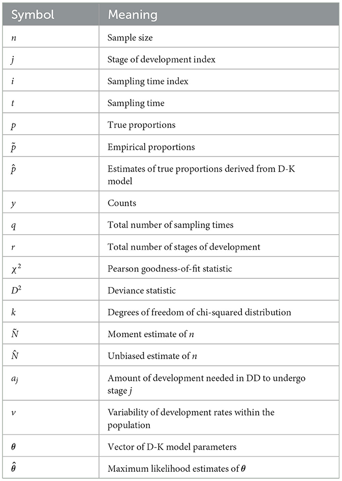
Table 1. Parameter nomenclature.

2 Estimation of sample size with known proportions

2.1 Purpose

This section describes a proposed method for estimating the unknown sample count n for a multinomial model with r possible outcomes, j = 1, 2, …, r, with known probabilities p₁, p₂, …, p_r. The count data y₁, y₂, …, y_r along with n are assumed missing, but data are present in the form of y_j/n.

2.2 Chi-square

For a multinomial model with r possible outcomes, and corresponding known probabilities p₁, p₂, …, p_r, drawing samples Y₁ = y₁, Y₂ = y = 2, …, Y_r = y_r, where $n={\displaystyle \sum _{j=1}^r}{y}_j$, have associated probability mass function:

$\begin{array}{ll}\text{P}(Y_1=y_1,Y_2=y_2,\dots ,Y_r=y_r)=\left(\frac{n!}{y_1!y_2!\dots y_r!}\right)p_1^{y_1}{p}_2^{y_2}\dots p_r^{y_r}.& (1)\end{array}$

We denote empirical proportions sampled from this distribution by ${\tilde{p}}_1,{\tilde{p}}_2,\dots ,{\tilde{p}}_r$.

The Pearson goodness-of-fit statistic for a multinomial with known group probabilities p₁, p₂, …, p_r can be written by factoring n out, thereby expressing the statistic in terms of known probabilities and empirical proportions (Equation 2):

$\begin{array}{ll}{\chi }^2=n{\displaystyle \sum _{j=1}^r}\frac{{({\tilde{p}}_j-p_j)}^2}{p_j}& (2)\end{array}$

or:

$\begin{array}{ll}{\chi }^2=n{D}^2.& (3)\end{array}$

As n becomes large, the sampling distribution of the Pearson statistic asymptotically approaches a chi-squared distribution with k degrees of freedom, k = r−1, and its variance asymptotically approaches the chi-squared distribution variance of 2k.

2.3 Method of moments

A method of moments estimate of the unknown parameter n is constructed by setting (χ²) equal to its expected value, the degrees of freedom k. The moment estimate of n follows from algebraic solution and is (𝔼(χ²)) divided by the deviance statistic, seen in Equation (4):

$\begin{array}{ll}Ñ=\frac{k}{D^2}.& (4)\end{array}$

The estimate increases as the deviance from chi-squared distribution decreases. Thus, the variability of the empirical proportions around the model proportions contains information for estimating n. The Pearson statistic was chosen for the basis of estimating n rather than the likelihood ratio statistic because the Pearson statistic is known to have superior asymptotic properties, such as for sparse tables [12]. For the purpose of evaluating the sampling distribution of Ñ, we rewrite it as follows:

$\begin{array}{ll}Ñ=\frac{nk}{{\chi }^2},& (5)\end{array}$

where (χ² ~)chi-squared(k). A chi-squared random variable divided by a constant has a gamma distribution, and Ñ is observed to be the reciprocal of a gamma random variable. In particular, Ñ = 1/Y where Y ~gamma(k/2, nk/2). The moment estimate Ñ is biased; the expected value of a reciprocal gamma provides a bias correction. If V has a gamma distribution with shape parameter α and rate parameter β (so that 𝔼(V) = α/β), then

$\begin{array}{ll}\text{𝔼}(\frac{1}{V})=\frac{\beta }{\alpha -1},& (6)\end{array}$

Thus from Equation (6), the expected value of the reciprocal of Y is as follows:

$\begin{array}{ll}\text{𝔼}(Ñ)=n\frac{k}{k-2}.& (7)\end{array}$

An unbiased estimate of n thus becomes:

$\begin{array}{ll}\widehat{N}=Ñ\frac{k-2}{k}.& (8)\end{array}$

A 100(1−γ)% confidence interval for n can be constructed from the relationship of the estimate $\widehat{N}$ with a chi-squared distribution. Given two chi-squared percentiles with PDF area 1−γ between them, the equal tail percentiles is as follows:

$\begin{array}{ll}\text{P}({\chi }_{1-\gamma /2}^2,{\chi }_{\gamma /2}^2)\approx 1-\gamma ,& (9)\end{array}$

An approximate 100(1−γ)% confidence interval for n is as follows:

$\begin{array}{ll}\text{P}({\chi }_{1-\gamma /2}^2,{\chi }_{\gamma /2}^2)=\left(\frac{{\chi }_{1-\gamma /2}^2\widehat{N}}{k-2},\frac{{\chi }_{\gamma /2}^2\widehat{N}}{k-2}\right).& (10)\end{array}$

2.4 Convergence of chi-squared

We studied the size n needed for the confidence interval coverage to hold true using iterative sampling from the multinomial distribution. Per each value of n, we performed 10⁴ times of iterative sampling and counted the proportion of confidence intervals that included n and compared that proportion with 1−γ.

Because the point and interval estimates of n were derived from the chi-squared goodness-of-fit statistic, we might expect the statistical properties of the estimates depend heavily on the adequacy of the chi-squared approximation. The conventional rules for the chi-squared statistic to asymptotically converge are for the expected counts e_j = np_j ≥ 5 for at least 80% of the cells and e_j ≥ 1 for all j [13]. Another common, more conservative, approach is setting e_j ≥ 5 for all j [14]. This leads to the conclusion that for higher probabilities, smaller sample sizes are adequate.

2.5 Results

We derive point estimates of n and actual coverage of 100(1−γ)% confidence interval for n using the method of moments, which was described earlier. In this example, we use true cell probabilities p₁, p₂, …, p_r, r = 6, with values of p = 〈1/12, 2/12, 3/12, 2/12, 2/12, 2/12〉 as an example. We chose a vector with low variability between cell probabilities to demonstrate when the method of moments approach works well, where, in next section, we build on technique to demonstrate method of moments estimation on the sparse dataset.

The values of n were set to 10, 50, 90, and 130. For each value of n, 10⁴ empirical counts Y₁ = y₁, Y₂ = y = 2, …, Y_r = y_r were drawn from a multinomial distribution (Equation 1). For each of 10⁴ empirical samples from the multinomial distribution, we obtained empirical proportions ${\tilde{p}}_1,{\tilde{p}}_2,\dots ,{\tilde{p}}_r$. The true probabilities and empirical proportions were then used to calculate point estimates of n (biased and unbiased) and 95% confidence intervals according to the Equation (10) and Table 2. For each of the iterations, we determined if the tested n value fell within the interval defined in the Equation (10). We report the total number of times it did in the percentage, which is defined as the $\widehat{\text{N}}$ empirical coverage of 95% CI. The chi-squared distribution approximation for Pearson's goodness-of-fit statistics is seen in Table 2 and Figure 1.

Table 2

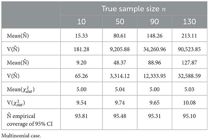
Table 2. Estimates of sample size parameters and empirical coverage of sample size from 10⁴ times of iterative sampling.

Figure 1

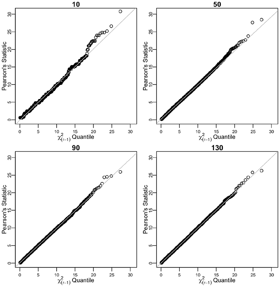
Figure 1. Sorted distances of Pearson's chi-squared statistic for varying n sample sizes (10, 50, 90, and 130) over 10⁴ times of iterative sampling plotted against the quantiles of $({\chi }_{r-1}^2)$ distribution. Multinomial case.

The unbiased estimate $\widehat{N}$ converges quickly to the true value n when p₁, p₂, …, p_r are non-sparse. When n is 50, approximately 83.33% of np_j ≥ 5, being at least 4, meets the requirements of minimum expected counts stated in the literature [13, 14]. The simulated biases of Ñ were considerable at 153.33%, 161.22%, 164.73%, and 163.93% of the n value for n of 10, 50, 90, and 130, respectively, close to nk/(k−2) as stated in Equation (7) for k = 5. The results of the mean value of (χ²) reciprocal over 10⁴ simulations are approximately 1/(k−2), and variance of approximately (2/[(k−2)²(k−4)]), the defined variance [15]. The asymptotic variance of Ñ is found from the reciprocal gamma variance as follows:

$\begin{array}{ll}\text{V}(Ñ)=n^2{k}^2\text{V}(\frac{1}{{\chi }^2})=\frac{2n^2{k}^2}{{(k-2)}^2(k-4)}.& (11)\end{array}$

The variance of Ñ from the iterative sampling, $sim=n^2{k}^2\mathrm{\text{V}}(1/{\chi }_{stat}^2)$, became closer to the asymptotic variance, asym from Equation (11) as n increased (|sim−asym|/asym) within 67.37%, 33.72%, 23.86%, and 3.58% of the asymptotic variance for n = 10, n = 50, n = 90, and n = 130, respectively.

3 Dennis–Kemp model with same n for each time interval

3.1 Purpose

This section implements on method for sample size n estimation described above and applies Dennis–Kemp model [3] for the implementation in forecasting plant development events of Blue Diamond Growers^® Nonpareil almonds. We present a method for the estimation of sample size; when probabilities of a crop being at a certain development stage are a function of degree-days, phenology dataset is recorded in percentages for each of r development stages and q sampling times, as well as how to account for sparseness of contingency tables due to low or zero expected cell probabilities.

3.2 Blue diamond almond counts

The Blue Diamond Growers^® keep track of development in almond orchards during each growing season for sampling times t_i, i = 1, 2, …, q in degree-days (DD) for r stages of tree development between dormancy and full bloom [8]. A project was initiated under the USDA Agricultural Research Service to develop a phenology model for the almonds in order to forecast the best time (10% bloom) to schedule honey bee placement for pollination. When the data were made available to USDA-ARS, the investigators became aware that the sampled proportions y_ij/n_i for each t_i, expressed as percentages, were recorded, but neither y_ij nor the n_i. Because the sampling protocol appeared to be standard, it was assumed that the sample size at each time t_i stayed the same, i.e., n_i = n.

3.3 Model description

We describe how the amount of development needed in DD to undergo stage j, j = 1, 2, …, r is derived from the maximization of the log-likelihood function of the Dennis–Kemp (D-K) model [1] as follows:

$\begin{array}{l}{p}_{ij}=1/[1+exp(-\frac{a_j-t_i}{\sqrt{\nu t_i}})]\text{, for}j=1\text{,}\\ p_{ij}=1/[1+exp(-\frac{a_j-t_i}{\sqrt{\nu t_i}})]-1/[1+exp(-\frac{a_{j-1}-t_i}{\sqrt{\nu t_i}})]\\ \text{, for}j=2,...,r-1\text{,}\\ p_{ij}=1-1/[1+exp(-\frac{a_{j-1}-t_i}{\sqrt{\nu t_i}})]\text{, for}j=r\text{.}& (12)\end{array}$

a_j represents the amount of development in DD needed to undergo stage j and ν is the variability of development rates within the population. The quantity a_j can be interpreted as the DD value at which half of the population is at stage j or an earlier stage. The model assumes the underlying development level of an organism to be a continuous mean-increasing stochastic process, with the organism entering a discernible stage j after attaining development level.

The log-likelihood for the Dennis–Kemp model can be expressed as a sum multinomial, noting that the first term is a constant (Equation 13):

$\begin{array}{ll}\begin{array}{l}\ell (\theta )={\displaystyle \sum _{i=1}^q\left(\begin{array}{c}n\\ y_{i1}{y}_{i2}\dots y_{ir}\end{array}\right)}+n{\displaystyle \sum _{i=1}^q{\displaystyle \sum _{j=1}^r{\tilde{p}}_{ij}\text{log}(p_{ij}),}}\hfill \end{array}& (13)\end{array}$

θ=〈a₁, a₂, …, a_r−1, ν〉. Here the log-likelihood is written under the assumption of the same sample size for each sampling time. Sample sizes n are not needed for maximization of θ.

The log-likelihood is maximized when the double sum is maximized. We derived the log ML parameter estimates $\widehat{\theta }$=$\langle {â}_1,{â}_2,\dots ,{â}_{r-1},\widehat{\nu }\rangle$ as described elsewhere [1] from the dataset (Figure 2 right). The data with q=18 sampling times originally consisted of r=7 development stages; Dormant, Green Tip, Pink Bud, Popcorn, Bloom, Petal Fall, Jacket. For all of the recorded sampling times, the dataset proportion was 0 for development stage j=1, corresponding to Dormant. The Dormant stage was excluded from the dataset, reducing the total number of stages of development to r=6.

Figure 2

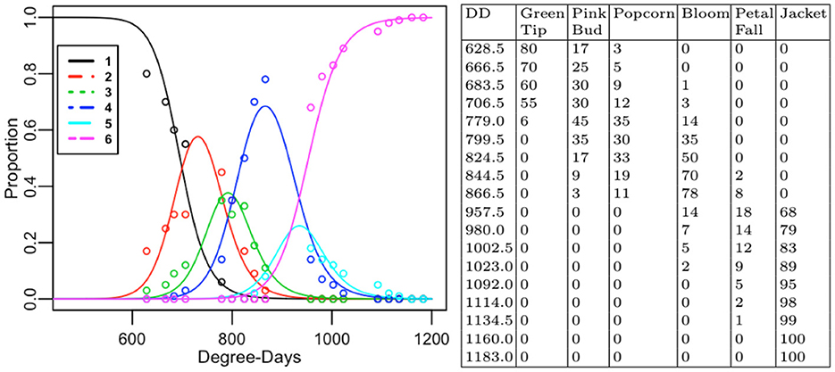
Figure 2. Line plots of estimates of expected proportions from the D-K model ${\widehat{p}}_{ij}$ in stages 1-6 as a function of temperature and time (Degree-Days). Colored circles correspond to proportions from the collected data, expressed in percentages (left). Contingency table showing the sparseness of collected proportions (right).

The estimates of expected proportions, ${\widehat{p}}_{i1},{\widehat{p}}_{i2},\dots ,{\widehat{p}}_{ir},i=1,2,\dots ,q$, were derived from the Dennis–Kemp model from Equation (12) with log ML estimates $\widehat{\theta }$, where $\widehat{\theta }$ = 〈695.593861, 769.75409, 816.23861, 919.06448, 952.97393, 1.08606〉. The (log) ML estimation makes it possible for the descriptive quality of the model to be evaluated for the collected (almond) dataset using the goodness-of-fit test. An estimate of the expected value for the collected dataset counts is $n{\widehat{p}}_{ij}$. The comparison of the fitted estimates of expected proportions as a function of DD from the Dennis–Kemp model against the observed proportions along with the two-way table with row percentages of Blue Diamond Growers^® Nonpareil almonds is shown in Figure 2.

3.4 Variability of maximum likelihood estimates depends on n

We derive the 100(1−γ)% Wald confidence interval for θ, of which the variance of the ML estimates depends on n. For sufficiently large samples, ML estimates $\widehat{\theta }$ follow a multivariate normal distribution with mean vector θ and variance-covariance matrix [13], seen in Equation (14):

$\begin{array}{ll}\text{V}(\theta )=\text{I}{(\theta )}^{-1},& (14)\end{array}$

where I(θ) is the Fisher information matrix for ℓ(θ), seen in Equation (15):

$\begin{array}{ll}\text{I}(\theta )=n{\displaystyle \sum _{i=1}^q}{\displaystyle \sum _{j=1}^r}\frac{1}{p_{ij}}\frac{\partial p_{ij}}{\partial {\theta }_k}\frac{\partial p_{ij}}{\partial {\theta }_l}.& (15)\end{array}$

The variance-covariance matrix V(θ) can be estimated with Hessian matrix $\mathrm{\text{J}}(\widehat{\theta })$ with r×r dimension for r parameters. The 100(1−γ)% Wald confidence interval for θ_j is seen in Equation (16):

$\begin{array}{ll}{\widehat{\theta }}_j\pm {\text{z}}_{\gamma /2}\sqrt{{\widehat{\text{v}}}_{jj}},& (16)\end{array}$

where ${\widehat{\mathrm{\text{v}}}}_{jj}$ is the j^th element on the main diagonal of $\widehat{\mathrm{\text{V}}}(\theta )$.

In Supplementary Table S1, we compare the variability of empirical ML estimates from empirical data sampled with different n values. In Section 3.5, we demonstrate the importance of the method of moments approach and its relation to Pearson goodness of fit statistic in the assessment of adequate n value for ML estimates from the D-K model, whereas in Section 3.6, we introduce the pooling method of sparse cells of $\widehat{p}$.

3.5 Estimation of n from method of moments

The sample size needed for confidence intervals of the Dennis–Kemp model ML is estimated with method of moments and its relation to Pearson goodness-of-fit statistic. From (χ² = nD²) (Equation 3), with a different (D²) than in previous section:

$\begin{array}{ll}{\chi }^2=n{\displaystyle \sum _{i=1}^q}{\displaystyle \sum _{j=1}^r}\frac{{({\tilde{p}}_{ij}-p_{ij})}^2}{p_{ij}},& (17)\end{array}$

where p_ij is estimated as ${\widehat{p}}_{ij}$ from the Dennis–Kemp model. From (χ²~)chi-squared(k):

$\begin{array}{ll}k=q(r-1)& (18)\end{array}$

which reflects the q sampling times, and the empirical proportions ${\tilde{p}}_{ij}$ are sampled from a product multinomial.

As derived in previous section in Equation (5), the moment estimate Ñ is biased, and $\widehat{N}$ in Equation (8) is the new unbiased estimate of n, with k = q(r−1). However, for the model with same r number of parameters, as the number of sampling times q increases, the bias of moment estimate Ñ decreases. For example, for r = 6, with a multinomial k = r−1 (equivalent to k = q(r−1) for q = 1), the expected value is 66.67%, which is too high, where with q = 18 sampling times, the sample size is overestimated only by 2.27%.

The 100(1−γ)% confidence interval for n with equal tail percentiles $(P({\chi }_{1-\gamma /2}^2,{\chi }_{\gamma /2}^2)\approx 1-\gamma )$ Equation (9) remains $(\text{P}({\chi }_{1-\gamma /2}^2,{\chi }_{\gamma /2}^2)=({\chi }_{1-\gamma /2}^2\widehat{N}/(k-2),{\chi }_{\gamma /2}^2\widehat{N}/(k-2)))$, as defined in Equation (10).

3.6 Convergence and low expected counts

The data contain zeroes for some of the development stages per t_i, and we propose a pooling technique. The convergence rule for a chi-squared statistic for product multinomial is same for a multinomial case; np_ij ≥ 1 for all j and np_ij ≥ 5 for at least 80% of the cells or more rigorous np_ij ≥ 5 for all j for each t_i separately. For our model with sparse data commonly observed in phenology, we allow np_ij < 1, otherwise pooling of cells per t_i would yield less than two cells per t_i. This is under the assumption that multinomial distributions for different times are assumed to be independent. Figure 3 illustrates the method.

Figure 3

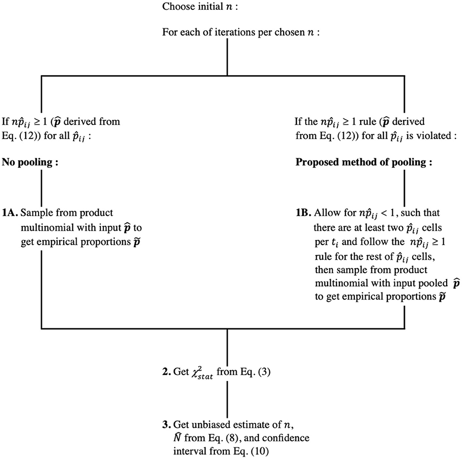
Figure 3. Proposed method of pooling of sparse $\widehat{p}$ to assess adequate sample size.

The estimated multinomial probabilities ${\widehat{p}}_{i1},{\widehat{p}}_{i2},\dots ,{\widehat{p}}_{ir}$ per t_i, i = 1, 2, …, q are found by maximization of vector θ, which have their lower bound set to equal to no less than a chosen constant (10⁻⁶). This allows for sampling of potentially non-zero empirical proportions ${\tilde{p}}_{i1},{\tilde{p}}_{i2},\dots ,{\tilde{p}}_{ir}$ for t₁, t₂, …, t_q. Sampled ${\tilde{p}}_{ij}$, for which a probability of random draw from multinomial distribution is set to the minimum value, will depend on that arbitrarily chosen lowest acceptable probability, leading to an extremely low value of that ${\tilde{p}}_{ij}$. A few low or zero counts can strongly bias sample size estimation. Pooling low expected probabilities ${\widehat{p}}_{i1},{\widehat{p}}_{i2},\dots ,{\widehat{p}}_{ir}$ together as a single stage [13] can be an alternative.

In the pooling case, instead of (χ²) holding q(r−1) degrees of freedom, each row of counts per t_i will contribute r_i−1 degrees of freedom, with r_i being not necessarily the same for i = 1, 2, …, q. Summation of r_i−1 over q sampling times yields new degrees of freedom k, which is distributed with $({\chi }_k^2)$:

$\begin{array}{ll}k={\displaystyle \sum _{i=1}^q}{r}_i-q.& (19)\end{array}$

The D² represented as a double sum in Equation (17) can be rewritten as Equation (20):

$\begin{array}{ll}{D}^2={\displaystyle \sum _{j=1}^{r_1}}\frac{{({\tilde{p}}_{ij}-p_{ij})}^2}{p_{ij}}+{\displaystyle \sum _{j=1}^{r_2}}\frac{{({\tilde{p}}_{ij}-p_{ij})}^2}{p_{ij}}+\cdots +{\displaystyle \sum _{j=1}^{r_q}}\frac{{({\tilde{p}}_{ij}-p_{ij})}^2}{p_{ij}}& (20)\end{array}$

Empirical sample size is derived by setting (𝔼(χ²)) to its expected degrees of freedom divided by the deviance statistic (Equation 21).

$\begin{array}{ll}Ñ=({\displaystyle \sum _{i=1}^q}{r}_i-q)/D^2.& (21)\end{array}$

The expected value of Ñ is defined by Equation (7) but with degrees of freedom from Equation (19). For the reciprocal of Ñ Y, Y~Γ(α, cβ) with

$\begin{array}{ll}c=nk& (22)\end{array}$

and

$\begin{array}{ll}\alpha =k/2,& (23)\end{array}$

(Equations 22, 23) the estimate of sample size n is corrected for bias and set to a new estimate $\widehat{N}$ (Equation 24).

$\begin{array}{ll}\widehat{N}=({\displaystyle \sum _{i=1}^q}{r}_i-q-2)/D^2.& (24)\end{array}$

3.7 Results

Following are the results of sample size estimation method with and without pooling the cells with low expected probabilities from the Dennis–Kemp model. The almond dataset consisted of 18 sampling times t_i, i = 1, 2, …, q, i.e., q = 18. The starting sample sizes were set to 50, 150, 250, and 500 before pooling and 50, 250, 750, and 1,000 with pooling. The parameters Ñ, $\widehat{N}$, and Pearson (χ²) and the coverages of $\widehat{N}$ were estimated from (10⁴) times of iterative sampling.

For the first case, the sample size estimation technique was evaluated for the unpooled model where the cell count per time point was kept constant at six for r = 6 stages of development of almond. The observed empirical proportions were sampled from a product multinomial. The Pearson (χ²) for 10⁴ times of iterative sampling was set to degrees of freedom k from Equation (18), with q = 18 and r = 6. The empirical coverages and variances of sample sizes derived from the method of moments are compared with the empirical coverages and variances of maximum likelihood estimates derived from the phenology model.

The second case involved pooling cells in the table with expected probabilities ${\widehat{p}}_{ij}$ so that each row that corresponded to specified t_i could potentially have different number of cells r_i. Following the cell pooling recommendations [13, 14], cells with ${\widehat{p}}_{ij}<$0.0035 were combined with adjacent ${\widehat{p}}_{ij}$ cells, except for last three sampling times, i = 16, i = 17, and i = 18, where cells were pooled with adjacent cell ${\widehat{p}}_{i5}=0.003488668$ for i = 16, ${\widehat{p}}_{i5}=0.0017957$ for i = 17, and ${\widehat{p}}_{i5}=0.0009966204$ for i = 18, respectively, so the table of pooled expected probabilities had at least two cells per sampling time t_i.

Sorted distances of Pearson's chi-squared statistic from 10⁴ times of iterative sampling were plotted against the quantiles of chi-squared distribution, ${\chi }_{q(r-1)}^2$ for first case (Table 3, Figure 4) and after pooling ${\chi }_k^2$, $k={\displaystyle \sum _{i=1}^q}{r}_i-q$, k = 51 for second case (Table 4, Figure 5).

Table 3

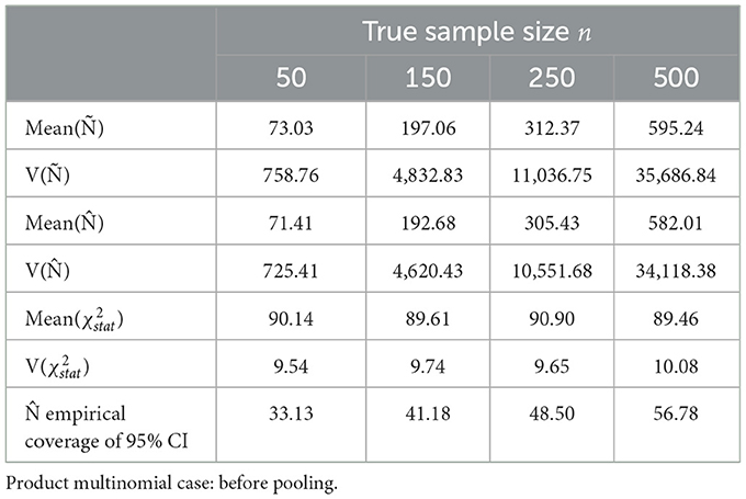
Table 3. Estimates of parameters and empirical coverage of sample size from 10⁴ times of iterative sampling.

Figure 4

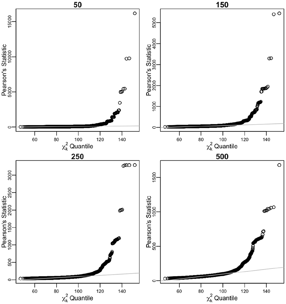
Figure 4. Sorted distances of Pearson's chi-squared statistic for varying n sample sizes (50, 150, 250, and 500) over 10⁴ times of iterative sampling plotted against the quantiles of ${\chi }_k^2$ distribution, k = q(r−1). Product multinomial before pooling case.

Table 4

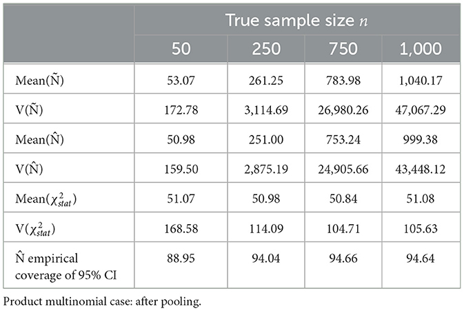
Table 4. Estimates of parameters and empirical coverage of sample size from 10⁴ times of iterative sampling.

Figure 5

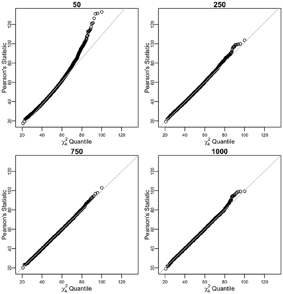
Figure 5. Sorted distances of Pearson's chi-squared statistic for varying n sample sizes (50, 250, 750, and 1,000) over 10⁴ times of iterative sampling plotted against the quantiles of ${\chi }_k^2$ distribution, $k={\displaystyle \sum _{i=1}^q}{r}_i-q$. Product multinomial after pooling case.

For n = 50, n = 150, n = 250, and n = 500 before pooling case, simulated biases of Ñ were considerable at 146.06%, 131.37%, 124.95%, and 119.05% of the n value, respectively, very slowly converging to nk/(k−2) (102.27% for k = 90), as stated in Equation (7). From the relationship of expected value of Ñ from Equation (11), the simulated variance of Ñ was within 1,147.71%, 783.01%, 625.96%, and 486.84% of the asymptotic variance for n = 50, n = 150, n = 250, and n = 500, respectively. The unbiased estimate $\widehat{N}$ converges slowly to n, and the $\widehat{N}$ empirical coverage of 95% CI is low (Table 3).

After pooling the sparse cells, the sample size estimation n improved. For n = 50, n = 250, n = 750, and n = 1, 000, the simulated biases of Ñ were considerable at 106.14%, 104.5%, 104.53%, and 104.02% of the n value, respectively (expected 104.08% for k = 51). For the same corresponding values of n, the simulated variance of Ñ was within 49.92%, 8.11%, 4.05%, and 2.10%, respectively of the asymptotic variance. The unbiased estimate $\widehat{N}$ converged quickly to n, and the $\widehat{N}$ empirical coverage of 95% CI was close to expected 95% (Table 4).

3.8 Discussion

In this study, we utilized the estimated sample size to construct confidence intervals of the population parameters using method of moments and pooling sparse data to estimate the sample size that converges to true coverage. The intended outcome is data sampling with adequate sample size to determine empirical estimates of population proportions. The goal is to predict the optimal timing to harvest crops at desired development stages when coupled with the phenology model.

We pooled our data such that $n{\widehat{p}}_{ij}\ge 1$ for all pooled cells, i.e., n = 286, when ${\widehat{p}}_{ij}\ge 0.0035$, except for last three out of eighteen rows to allow for two cells in these rows. We showed that the variability of the ML estimates depends on the sample size, but the maximum-likelihood method is not adequate to assess the sample size through the convergence of empirical coverage of $\widehat{\theta }$. We showed that without pooling case, the empirical variance of sample size was over 400% of the asymptotic variance and that the coverage of sample size was low, even at n = 500. For the pooling case, we observed a dramatic drop from 49.92% at n = 50 to below 10% in the empirical variance of sample size when n reached 250 and below 5% in the empirical variance of sample size when n reached 750. It is recommended that the rule for pooling is not violated more than the tested limit. The proposed method is an improvement over the existing technique [16] that does not allow exceptions to the pooling. It is also more relevant than the method proposed by Otis et al. [11] for mark-recapture in closed populations.

The developed model is an extension from the Dennis–Kemp model [1], in which the maximization of parameter estimates does not depend on the sample size but their variability does. The expected proportions of almond data are a function of temperature and time, and the implementation of developed sample size estimation with previously developed models can be applied to future phenology data.

The rationale for choosing 10⁴ as the number of iterations in our analysis was to optimize the high computational time associated with the likelihood maximization and the statistical assessment of empirical data. In the future, we will perform a more robust analysis with a larger number of iterations, during which we will explore the performance of the method with other confidence intervals, in addition to the Wald interval, including the Wilson score interval.

For Blue Diamond Growers^® almond data, an assumption of our technique proposed in this study is that constant sample size over sampling time individual multinomials for each t_i is assumed to be independent [13]. Future expansion of this technique is to incorporate a non-product multinomial technique to account for time dependency and allow for variable sample sizes per t_i. A thorough knowledge of the studied population is needed for the assumption to be deemed feasible.

Data availability statement

The original contributions presented in the study are included in the article/Supplementary material, further inquiries can be directed to the corresponding author.

Author contributions

ML: Conceptualization, Data curation, Investigation, Methodology, Software, Validation, Visualization, Writing – original draft, Writing – review & editing. BD: Conceptualization, Data curation, Funding acquisition, Investigation, Project administration, Resources, Software, Supervision, Writing – original draft, Writing – review & editing.

Funding

The author(s) declare financial support was received for the research, authorship, and/or publication of this article. This work was supported by US Department of Agriculture (http://www.ars.usda.gov/main/site_main.htm?modecode=30-00-00-0058-5442-2-327) to BD.

Conflict of interest

The authors declare that the research was conducted in the absence of any commercial or financial relationships that could be construed as a potential conflict of interest.

Publisher's note

All claims expressed in this article are solely those of the authors and do not necessarily represent those of their affiliated organizations, or those of the publisher, the editors and the reviewers. Any product that may be evaluated in this article, or claim that may be made by its manufacturer, is not guaranteed or endorsed by the publisher.

Supplementary material

The Supplementary Material for this article can be found online at: https://www.frontiersin.org/articles/10.3389/fams.2024.1374832/full#supplementary-material

References

1. Dennis B, Kemp WP, Beckwith RC. Stochastic model of insect phenology: estimation and testing. Environ Entomol. (1986) 15:540–6. doi: 10.1093/ee/15.3.540

PubMed Abstract | Crossref Full Text | Google Scholar

2. World Agricultural Supply and Demand Estimates. Technical report. United States Department of Agriculture (2018).

Google Scholar

3. Kemp WP, Dennis B, Beckwith RC. Stochastic phenology model for the western spruce budworm (Lepidoptera: Tortricidae). Environ Entomol. (1986) 15:547–54. doi: 10.1093/ee/15.3.547

PubMed Abstract | Crossref Full Text | Google Scholar

4. Dennis B, Kemp WP. Further statistical inference methods for a stochastic model of insect phenology. Environ Entomol. (1988) 17:887–93. doi: 10.1093/ee/17.5.887

Crossref Full Text | Google Scholar

5. Bishop YM, Fienberg SE, Holland PW. Discrete Multivariate Analysis: Theory and Practice. New York, NY: Springer Science & Business Media. (2007).

PubMed Abstract | Google Scholar

6. Candy SG. Modeling insect phenology using ordinal regression and continuation ratio models. Environ Entomol. (1991) 20:190–5. doi: 10.1093/ee/20.1.190

PubMed Abstract | Crossref Full Text | Google Scholar

7. Candy SG. Predicting time to peak occurrence of insect life-stages using regression models calibrated from stage-frequency data and ancillary stage-mortality data. Agric For Entomol. (2003) 5:43–9. doi: 10.1046/j.1461-9563.2003.00161.x

Crossref Full Text | Google Scholar

8. Bloom/Harvest Reports. Blue Diamond Almonds Growers (2005–2021). Available online at: http://www.bdingredients.com/category/almond-bloom-harvest-reports/ (accessed February 21, 2024).

Google Scholar

9. Eichenberger P, Hulliger B, Potterat J. Two measures for sample size determination. In: Survey Research Methods. (2011). p. 27–37.

Google Scholar

10. Thompson SK. Sample size for estimating multinomial proportions. Am Stat. (1987) 41:42–6. doi: 10.1080/00031305.1987.10475440

Crossref Full Text | Google Scholar

11. Otis DL, Burnham KP, White GC, Anderson DR. Statistical inference from capture data on closed animal populations. Wildlife Monogr. (1978) 62:3–135.

Google Scholar

12. Read TR, Cressie NA. Goodness-of-Fit Statistics for Discrete Multivariate Data. New York, NY: Springer Science & Business Media. (2012).

Google Scholar

13. Tamhane A, Dunlop D. Statistics and Data Analysis: From Elementary to Intermediate. Upper Saddle River, NJ: Prentice Hall. (2000).

Google Scholar

14. Samaniego FJ. Stochastic Modeling and Mathematical Statistics: a Text for Statisticians and Quantitative Scientists. Boca Raton, FL: CRC Press. (2014). doi: 10.1201/b16414

Crossref Full Text | Google Scholar

15. Bernardo JM, Smith AF. Bayesian Theory. vol 405 Hoboken, NJ: John Wiley & Sons. (2009).

Google Scholar

16. Bresnahan JL, Shapiro MM. A general equation and technique for the exact partitioning of chi-square contingency tables. Psychol Bull. (1966) 66:252. doi: 10.1037/h0023728

PubMed Abstract | Crossref Full Text | Google Scholar