Understanding COVID-19 propagation: a comprehensive mathematical model with Caputo fractional derivatives for Thailand

This research introduces a sophisticated mathematical model for understanding the transmission dynamics of COVID-19, incorporating both integer and fractional derivatives. The model undergoes a rigorous analysis, examining equilibrium points, the reproduction number, and feasibility. The application of fixed point theory establishes the existence of a unique solution, demonstrating stability in the model. To derive approximate solutions, the generalized Adams-Bashforth-Moulton method is employed, further enhancing the study's analytical depth. Through a numerical simulation based on Thailand's data, the research delves into the intricacies of COVID-19 transmission, encompassing thorough data analysis and parameter estimation. The study advocates for a holistic approach, recommending a combined strategy of precautionary measures and home remedies, showcasing their substantial impact on pandemic mitigation. This comprehensive investigation significantly contributes to the broader understanding and effective management of the COVID-19 crisis, providing valuable insights for shaping public health strategies and guiding individual actions.

1 Introduction

The novel coronavirus, later identified as SARS-CoV-2, was first reported in Wuhan, China, in December 2019. Investigations suggested that the virus may have originated in bats and was potentially transmitted to humans through an intermediate host, possibly from a wild animal traded at a seafood market in Wuhan. Zoonotic diseases, where pathogens jump from animals to humans, are not uncommon, and past infectious disease outbreaks have similarly had zoonotic origins. Examples include the H1N1 influenza virus, Ebola virus, and Middle East Respiratory Syndrome (MERS) coronavirus. These viruses undergo genetic mutations or reassortment, enabling them to adapt and infect humans. Studying the origins of such diseases is crucial for prevention and control, and ongoing international research aims to comprehend the circumstances leading to the initial transmission of SARS-CoV-2 to humans Mathematical models play an important role in understanding the transmission dynamics of diseases, providing policymakers with a valuable tool for assessing and evaluating potential health risks.

Mathematical modeling in epidemiology plays a crucial role in understanding and predicting the spread of infectious diseases within populations. By employing mathematical equations and statistical techniques, epidemiologists can simulate the dynamics of disease transmission, assess the impact of interventions, and formulate informed public health strategies. These models often consider factors such as the rate of infection, recovery, and contact between individuals to simulate the progression of an outbreak. Through mathematical modeling, researchers can explore different scenarios, evaluate the Impact of various control measures, and ultimately contribute to the development of evidence-based policies targeted at mitigating the influence of infectious diseases on society. Mathematical models in epidemiology serve as powerful tools for decision-makers in their efforts to prevent, manage, and regulate the transmission of disease in society. Indeed, mathematical modeling has been extensively applied to study various infectious diseases, including malaria, chickenpox, and COVID-19. Each disease presents unique challenges, and mathematical models help researchers and public health officials understand the dynamics of transmission, evaluate the impact of interventions, and make informed decisions. For malaria, models might focus on factors like mosquito breeding habitats, vector behavior, and the impact of insecticide-treated bed nets. In the case of chickenpox, models may consider the age structure of the population and the waning immunity over time. The COVID-19 pandemic has witnessed a surge in mathematical modeling efforts to predict the course of the disease, evaluate the influence of non-pharmaceutical interventions, and guide vaccination strategies. These models provide valuable insights that aid policymakers in designing strategies to control and prevent the spread of contagious diseases. In 2023, the study examined the effectiveness of precautionary measures in managing chickenpox in Phuket by utilizing mathematical modeling and conducting bifurcation analysis to evaluate potential outcomes [1], and also in Jose et al. [2] the authors have developed and analyzed a deterministic mathematical model to investigate the transmission dynamics of co-infection involving Dengue Fever (DF) and Zika virus (ZIKV), also Van den Driessche and Watmough [3] presents a two-strain epidemic mathematical model that incorporates vaccination strategies, as discussed in the journal Computer Methods in Biomechanics and Biomedical Engineering and also in Joseph et al. [4] discusses a fractional-order density-dependent mathematical model aimed at identifying the superior strain of Wolbachia, available as an open access article with options for ordering article reprints and citations. Similarly in 2022, a stuy focused on the computational dynamics of a fractional order substance addictions transfer model incorporating the Atangana-Baleanu-Caputo derivative was conducted [5]. And Thomas et al. [6] delves into modeling and analyzing SEIRS epidemic models, specifically focusing on the 2019-nCoV outbreak in India, utilizing the homotopy perturbation method. In 2022, Jose et al. [7] conducts stability analysis and a comparative study on various eco-epidemiological models, particularly focusing on impulsive control strategies, with a stage structure considered for both prey and predator dynamics and the study in Jose et al. [8] explores the impact of strong determination and awareness on substance addictions through a mathematical modeling approach.

After exposure to the virus, symptoms typically manifest in individuals within a range of two to 14 days. The insidious nature of the coronavirus reveals a concerning aspect as individuals harboring the virus may become contagious up to 48 h before symptoms materialize. This contagious phase extends for a variable span of 10 to 20 days, influenced by the intricacies of one's immune response and the severity of the illness. The initial signs of the virus present a diverse array of symptoms, encompassing the familiar culprits such as cough, fever, and shortness of breath. However, the subtlety lies in the nuanced manifestations including, muscle aches, sore throat, loss of taste or smell, and a range of other discomforts. This temporal intricacy and symptomatic diversity underscore the challenges in identifying and containing the spread of the virus effectively. COVID-19 can manifest as mild illness in some individuals, while others may remain asymptomatic. In severe cases, the disease can lead to respiratory distress. Lingering impact resonates within, leaving lasting impressions on the lungs, heart muscles, and intricacies of the nervous system. Renal failure or, in extreme instances, death.

The detailed study of disease momentum is a prevailing theme for many mathematicians and biologists. We can observe numerous works, such as those by Haq et al. [9], Koca [10], and Rida et al. [11]. Many researchers have explored the extensions of mathematical models into fractional dimensions from their original integer order, representing genuine data in a proficient manner, as evidenced in the approaches of Akbari Kojabad and Rezapour [12], Talaee et al. [13], and Qureshi [14]. In recent years, numerous papers have delved into the intricacies of the Caputo-Fabrizio fractional derivative, similar to works by Ali Dokuyucu et al. [15] and Koca [10]. Moreover, in recent years, a multitude of published works based on the fractional derivative, such as Jan et al. [16–18], and Alharbi et al. [19] have emerged. Also in 2021, a paper was published, presenting a predictive model for breast cancer that integrates tolerance-based intuitionistic fuzzy-rough set feature selection with artificial neural network (ANN) algorithms [20], and a paper regarding the analysis of a novel coronavirus model (COVID-19) through the lens of the Caputo-Fabrizio fractional operator represents a pioneering endeavor in applied and computational mathematics [21]. The primary purpose of employing a mathematical model is to simulate the intricate dynamics of disease transmission, with a particular focus on ailments such as coronavirus disease. We can explore a myriad of paper-related topics in fractional calculus, such as Shah et al. [22], Jan et al. [23], Tang et al. [24], Jan et al. [25], Jan et al. [26] Jan et al. [27], and Anggriani et al. [28].

The fractional-order derivative is a broader interpretation, extending beyond the conventional scope of the integer-order derivative. The Caputo fractional derivate has been chosen not only because of its capability to integrate the memory effect on the model but also the completeness of the analytical tools to provide the dynamical behaviors of the model which does not exist on the other fractional derivative such as the Caputo-Fabrizio [29, 30] and Atangana-Baleanu [31] operators. In recent years, fractional-order derivatives have demonstrated superior performance in mathematical modeling compared to other approaches. Therefore, our focus is on investigating the transmission model of COVID-19 utilizing the Caputo fractional-order derivative. Given the global pervasiveness of COVID-19 and its status as the latest global disease, we aim to present predictions based on published statistical and numerical information. Considering that limiting interpersonal interactions in the community is one of the strategies for epidemic control, our study explores the influence of the proportion of contact between infected and wholesome individuals on the circulation of COVID-19.

From a mathematical standpoint, the diffusion of the disease is expected to reduce when the effective reproduction number remains bounded by 1. Additionally, a research on controlling the Spread mechanisms of a virus has been proposed by Edward et al. [32] using a mathematical model. De la Sen et al. [33] presented a novel SEIR epidemic model to investigate the impact of double-dose vaccination feedback. In their study in 2022, Gomes et al. [34] examined the role of the vaccine in contributing to the establishment of immunity in individuals in a population. In 2020, Annas et al. [35] developed a COVID-19 model to investigate the spread of the virus, incorporating factors such as vaccination and isolation. Additionally, in 2021, Moore et al. [36] utilized a certain mathematical model to measure the influence of the vaccine in supervising the sustained momentum of coronavirus.

The study of COVID-19 transmission in Thailand is pivotal in predicting the spread of the disease, offering invaluable insights for estimating healthcare resource requirements such as hospital beds, ventilators, and medical staff. By comprehensively analyzing transmission rates, incubation periods, and the effectiveness of public health interventions, this research illuminates strategies to curtail further spread and maintain control over the outbreak. Through identifying patterns of virus transmission, including peak infection periods and potential hot spots, the study provides essential guidance for mitigation efforts. Moreover, it enhances our understanding of the multifaceted factors influencing viral spread, empowering us to make informed decisions. Utilizing metrics like the reproduction number, we can forecast future transmission rates with greater accuracy. Notably, recognizing the impact of various parameters in the model is crucial, as it can significantly alter outcomes, underscoring the importance of precision in pandemic modeling and response strategies.

This paper is divided into several sections. Second section provides fundamental definitions and concepts of calculus in fractions. In Section 3, we delve into the fractional model of COVID-19 transmission. The discussion of the uniqueness and existence of the solution is presented in Section 4. Finally, Section 5 outlines the numerical method employed for solving the model, accompanied by the presentation of numerical results.

The main highlights:

• Novel mathematical model incorporating integer and fractional derivatives:

The study introduces a unique mathematical model for COVID-19 transmission that goes beyond traditional models by incorporating both integer and fractional derivatives. This innovation allows for a more accurate representation of the complex dynamics involved in the spread of the virus.

• Evaluation of equilibrium points and reproduction number:

The research conducts a thorough analysis of the mathematical model, specifically examining equilibrium points and the reproduction number. This provides a deeper understanding of the stability and characteristics of the system, offering insights into critical aspects of COVID-19 transmission dynamics.

• Establishment of existence of a unique solution using fixed point theory:

The study employs fixed point theory to rigorously establish the occurrence of a unique solution to the proposed mathematical model. This contributes to the mathematical foundation of the model and enhances confidence in its predictive capabilities, demonstrating the robustness of the approach.

• Application of the generalized adams-bashforth-moulton method for approximate solutions:

The research utilizes the generalized Adams-Bashforth-Moulton method to obtain estimated solutions for the mathematical model. This computational technique allows for practical implementation and analysis, facilitating the exploration of the model's behavior and outcomes.

• Real-world application through numerical simulation with Thailand's data: The study goes beyond theoretical developments by applying the mathematical model to real-world scenarios. A numerical simulation based on data from Thailand is conducted, offering a practical examination of COVID-19 transmission dynamics. This application provides valuable insights into the specific context of the pandemic, including data analysis and parameter estimation.

2 Model formation

In this model, individuals can be categorized into six groups: susceptible individuals (S), exposed individuals (E), quarantined individuals(Q), symptomatic infected individuals (I), asymptomatic infected individuals (A), and removed individuals (R), including cured and dead individuals. In the SEQIAR epidemiological model, the quarantine compartment plays a crucial role in representing individuals who have been exposed to the infectious agent but are temporarily isolated from the general population. The Quarantine compartment accounts for those who have closely interacted with individuals carrying the infection and are placed under quarantine to avoid the potential spread of the disease. This compartment acknowledges the incubation period during which individuals may not yet exhibit symptoms but can transmit the infection. The inclusion of a quarantine compartment enhances the SEIAR model's realism by capturing the impact of public health measures, such as isolation and quarantine, in controlling the transmission of infectious illness. Through the incorporation of the quarantine compartment, the SEQIAR model becomes a valuable tool for emulating and understanding the momentum of epidemics and assessing the effectiveness of interventions in mitigating disease transmission. The entire population is represented by N, where N = S + E + Q + I + A + R this model is represented as below;

$\begin{array}{l}\frac{dS}{dt}=\Lambda -\mu S-\frac{\alpha S((I+xA))}{N},\\ \frac{dE}{dt}=\frac{\alpha S((I+xA))}{N}-(\theta +\gamma +\mu )E,\\ \frac{dQ}{dt}=\gamma E-(\varphi +\mu +{\mu }_1+\psi +{\psi }_1)Q,\\ \frac{dA}{dt}=\sigma \theta E+\pi \varphi Q-({\chi }_1+\mu +{\mu }_2)A,\\ \frac{dI}{dt}=(1-\sigma )\theta E+(1-\pi )\varphi Q-(\mu +{\mu }_3+{\chi }_2)I,\\ \frac{dR}{dt}={\chi }_{1}A+{\chi }_{2}I+(\psi +{\psi }_1)Q-\mu R,& (1)\end{array}$

with,

S(0) = S₀, E(0) = E₀, I(0) = I₀, A(0) = A₀, Q(0) = Q₀ are the initial conditions of the system.

Referencing the detailed provided in Table 1, one can find an exhaustive compilation of the parameters alongside their comprehensive descriptions, facilitating a thorough understanding of the system's intricacies.

Table 1

Table 1. Detailed description of parameters of the model (Equation 1).

3 Quantitative evaluation of the model

In this section, we've examined the invariant region, the positivity of the solution, the presence of equilibria, disease-free and disease-endemic equilibrium points, the basic reproduction number and also conducted stability analysis.

3.1 Positive invariance

Using the following theorem we can demonstrate the nonnegativity,

Theorem 3.1. Solutions of the all dynamic attribute (S(t),E(t),Q(t),A(t),I(t),R(t)) with initial condition satisfy S(t) > 0, E(t) > 0, Q(t) > 0, A(t) > 0, I(t) > 0, R(t) > 0 for every t > 0, then the system (Equation 1) is positively invariant

Proof. now choose the equation of $\frac{dS}{dt}$ from the system (Equation 1),

$\begin{array}{l}\frac{dS}{dt}=\Lambda -\mu S-\frac{\alpha S(I+xA)}{N}\\ \frac{dS}{dt}=\Lambda -yS\end{array}$

where,

$\begin{array}{l}y=\mu +\frac{\alpha (I+xA)}{N}\end{array}$

Now, we get the following expression from integrating the above equation

$\begin{array}{l}S(t)=S_{0}exp(-{\displaystyle {\int }_0^t}y(v)dv)+\Lambda exp(-{\displaystyle {\int }_0^t}y(v)dv)\\ S(t)\ge S_{0}exp(-{\displaystyle {\int }_0^t}y(v)dv)>0\end{array}$

Now we can show the positive invariance for all variables

$\begin{array}{l}\frac{dE}{dt}=\frac{\alpha (I+xA)}{N}-(\theta +\gamma +\mu )E\\ \frac{dE}{dt}\ge -(\theta +\gamma +\mu )E\end{array}$

by integrating the above equation, we get

$\begin{array}{l}E(t)\ge E_{0}exp(-{\displaystyle {\int }_0^t}(\theta +\gamma +\mu )dv)>0\\ Q(t)\ge Q_{0}exp(-{\displaystyle {\int }_0^t}(\varphi +\mu +{\mu }_1+\psi +{\psi }_1)dv)>0\\ A(t)\ge A_{0}exp(-{\displaystyle {\int }_0^t}({\chi }_1+\mu +{\mu }_2)dv)>0\\ I(t)\ge I_{0}exp(-{\displaystyle {\int }_0^t}(\mu +{\mu }_3+{\chi }_2)dv)>0\\ R(t)\ge R_{0}exp(-{\displaystyle {\int }_0^t}\mu dv)>0\end{array}$

Hence the proof.

3.2 Boundedness

We examined the model (Equation 1) to obtain the a biologically feasible solution set. now, the following theorem assures that the system's solutions find their realm within a specified set, elegantly abiding by conditions of non-negativity.

Theorem 3.2. The set of feasible solution of the system of Equation 1 with the initial conditions which initiate in $R_{+}^6$ are bounded uniformly in Δ, where Δ = (S, E, Q, A, I, R) belongs $R_{+}^6:S+E+Q+A+I+R=N$ is the positively invariant region.

Proof. By using the non-negative initial conditions in the system (Equation 1), it is noticed that each of the Varying parameter remains non-negative, by Theorem 3.1. Now, when we sum each equation in Equation 1 to determine the overall population size, N(t), one must consider the scenario where there are no fatalities attributed to COVID-19.

$\begin{array}{l}\frac{dN}{dt}=\frac{dS}{dt}+\frac{dE}{dt}+\frac{dQ}{dt}+\frac{dA}{dt}+\frac{dI}{dt}+\frac{dR}{dt}\\ \Rightarrow \frac{dN}{dt}=\mu N-\mu S-\mu E-\mu Q-{\mu }_{1}Q-\mu A-\\ {\mu }_{2}A-\mu I-{\mu }_{3}I-\mu R\\ \Rightarrow \frac{dN}{dt}=0\end{array}$

Upon integration of the aforementioned equation, the result is obtained as, N(t) is a constant.

Accordingly, with the constant magnitude of the population, we obtain that all feasible solutions of each of the system of Equation 1 with variable parameters i.e., S,E,Q,A,I, and R are bounded in the invariant region.

3.3 Evaluation of equilibrium points and its stability

In examining the transmission of an infection, the disease-free equilibrium (DFE) represents a population state crucial for understanding when the disease is not widespread. The determination of the disease-free equilibrium involves setting E, Q, A, I, and R to zero in the system of Equation 1. Therefore, the disease-free equilibrium for model (Equation 1) is characterized by the following system of equations being satisfied:

$\begin{array}{l}\frac{dS}{dt}=\frac{dE}{dt}=\frac{dQ}{dt}=\frac{dA}{dt}=\frac{dI}{dt}=\frac{dR}{dt}=0\end{array}$

The solution to the algebraic equations allows us to identify the system's equilibrium points. The disease-free equilibrium point is reached when the absence of any ailment prevails, given by $E^0=(\frac{\Lambda }{\mu },0,0,0,0,0)$.

And also, if R₀ > 1, then the system (Equation 1) also has a positive endemic equilibrium $E_1^{*}=(S^{*},E^{*},I^{*},A^{*},R^{*},Q^{*})$,

$\begin{array}{l}{E}^{*}=\frac{\varphi +\mu +{\mu }_1+\psi +{\psi }_1}{\gamma }{Q}^{*}\\ A^{*}=\frac{\sigma \theta \varphi +\sigma \theta \mu +\sigma \theta {\mu }_1+\sigma \theta \psi +\sigma \theta {\psi }_1+\gamma \pi \varphi }{\gamma {\chi }_1+\gamma \mu +\gamma {\mu }_2}{Q}^{*}\\ I^{*}=\frac{\begin{array}{c}\varphi +\mu +{\mu }_1+\psi +{\psi }_1-\sigma \theta \varphi -\sigma \theta \mu -\sigma \theta {\mu }_1-\sigma \theta \psi \\ -\sigma \theta {\psi }_1+\theta \gamma -\pi \varphi \gamma \end{array}}{\gamma \mu +\gamma {\mu }_3+\gamma {\chi }_2}{Q}^{*}\\ R^{*}=\frac{{\chi }_1\beta +{\chi }_2\delta +(\psi +{\psi }_1)}{\mu }{Q}^{*}\\ S^{*}=\frac{(\theta +\gamma +\mu )N\kappa }{\alpha (\delta +\beta x)}\\ Q^{*}=\frac{\Lambda -\mu \upsilon }{\alpha \upsilon (\delta +\beta x)}\end{array}$

where,

$\begin{array}{l}\beta =\frac{\sigma \theta \varphi +\sigma \theta \mu +\sigma \theta {\mu }_1+\sigma \theta \psi +\sigma \theta {\psi }_1+\gamma \pi \varphi }{\gamma {\chi }_1+\gamma \mu +\gamma {\mu }_2}\\ \delta =\frac{\begin{array}{c}\varphi +\mu +{\mu }_1+\psi +{\psi }_1-\sigma \theta \varphi -\sigma \theta \mu -\sigma \theta {\mu }_1-\sigma \theta \psi \\ -\sigma \theta {\psi }_1+\theta \gamma -\pi \varphi \gamma \end{array}}{\gamma \mu +\gamma {\mu }_3+\gamma {\chi }_2}\\ \kappa =\frac{\varphi +\mu +{\mu }_1+\psi +{\psi }_1}{\gamma }\\ \upsilon =\frac{(\theta +\gamma +\mu )N\kappa }{\alpha (\delta +\beta x)}\end{array}$

The stability of E⁰ relies on the basic reproductive number R₀, which represents the average number of secondary cases generated by a COVID-19 infected individual throughout their contagious period when introduced to a population of susceptible individuals without any interventions. We examine the equilibrium's stability using the next-generation operator. Referring to the notations in Van den Driessche and Watmough [3] for model (Equation 1), the matrices F, representing new infections, and V, representing the remaining transfer terms, are provided as follows.

$\begin{array}{l}F=\left[\begin{array}{c}\frac{\alpha S(t)((I(t)+xA(t))}{N}\\ 0\\ 0\\ 0\end{array}\right]\end{array}$

and

$\begin{array}{l}V=\left[\begin{array}{c}(\theta +\gamma +\mu )E(t)\\ -\gamma E(t)+(\varphi +\mu +{\mu }_1+\psi +{\psi }_1)Q(t)\\ -\sigma \theta E(t)-\pi \varphi Q(t)+({\chi }_1+\mu +{\mu }_2)A(t)\\ -(1-\sigma )\theta E(t)-(1-\pi )\varphi Q(t)+(\mu +{\mu }_3+{\chi }_2)I(t)\end{array}\right]\end{array}$

The Jacobian matrix for F and V at E₀ obtained as

$\begin{array}{l}{J}_F(E_0)=\left[\begin{array}{cccc}0& 0& \alpha x\frac{\Lambda }{\mu N}& \alpha \frac{\Lambda }{\mu N}\\ 0& 0& 0& 0\\ 0& 0& 0& 0\\ 0& 0& 0& 0\end{array}\right]\end{array}$

and

$\begin{array}{l}{J}_V(E_0)\\ ={\lambda }^{\eta -1}\left[\begin{array}{cccc}\theta +\gamma +\mu & 0& 0& 0\\ -\gamma & \varphi +\mu +{\mu }_1+\psi +{\psi }_1& 0& 0\\ -\sigma \theta & -\pi \varphi & {\chi }_1+\mu +{\mu }_2& 0\\ -(1-\sigma )\theta & -(1-\pi )\varphi & 0& \mu +{\mu }_3+{\chi }_2\end{array}\right]\end{array}$

FV⁻¹ is known as the next generation matrix for the system, then the basic reproduction number is defined as $R_0=\rho (F{V}^{-1}),$ i.e.,

$\begin{array}{l}\frac{\alpha x\Lambda (\theta \sigma (\varphi +\mu +{\mu }_1+\psi +{\psi }_1))}{\mu N(\theta +\mu +\gamma )(\varphi +\mu +{\mu }_1+\psi +{\psi }_1)({\chi }_1+\mu +{\mu }_2)}\\ +\frac{\alpha \Lambda (\gamma (1-\pi )\varphi +(\varphi +\mu +{\mu }_1+\psi +{\psi }_1)(1-\sigma )\theta )}{\mu N(\theta +\mu +\gamma )(\varphi +\mu +{\mu }_1+\psi +{\psi }_1)(\mu +{\mu }_3+{\chi }_2)}\end{array}$

3.4 Stability analysis of the equilibrium point

Theorem 3.3. The disease-free equilibrium, $E^0=(S^0,0,0,0,0,0)=(\frac{\Lambda }{\mu },0,0,0,0,0)$, of the system (Equation 1) is globally asymptotically stable if R₀ < 1 and unstable if R₀ > 1.

Proof. We consider the following Lyapunov functional L₀ as in Yaagoub et al. [37], given by

$\begin{array}{l}{L}_0=S^0\left(\frac{S}{S^0}-ln\left(\frac{S}{S^0}\right)-1\right)+E+\frac{(\theta +\gamma +\mu )}{\gamma }Q\\ +\frac{(\varphi +\mu +{\mu }_1+\psi +{\psi }_1)(\theta +\gamma +\mu )}{\gamma \pi \varphi }A\\ +\frac{(\varphi +\mu +{\mu }_1+\psi +{\psi }_1)(\theta +\gamma +\mu )}{\gamma (1-\pi )\varphi }I.& (2)\end{array}$

Then,

$\begin{array}{l}{\dot{L}}_0\le \left(1-\frac{S}{S^0}\right)+Ė+\frac{(\theta +\gamma +\mu )}{\gamma }\dot{Q}\\ +\frac{(\varphi +\mu +{\mu }_1+\psi +{\psi }_1)(\theta +\gamma +\mu )}{\gamma \pi \varphi }Ȧ\\ +\frac{(\varphi +\mu +{\mu }_1+\psi +{\psi }_1)(\theta +\gamma +\mu )}{\gamma (1-\pi )\varphi }İ.\end{array}$

Then, after calculation, we will have

$\begin{array}{l}{\dot{L}}_0\le \mu S^0\left(2-\frac{S}{S^0}-\frac{S^0}{S}\right)\\ +\frac{\left(\theta +\gamma +\mu \right)\left(\varphi +\mu +{\mu }_1+\psi +{\psi }_1\right)\left({\chi }_1+\mu +{\mu }_2\right)}{\gamma \pi \varphi }\\ \left(\frac{\alpha S^0\gamma \pi \varphi }{N\left(\theta +\gamma +\mu \right)\left(\varphi +\mu +{\mu }_1+\psi +{\psi }_1\right)\left({\chi }_1+\mu +{\mu }_2\right)}-1\right)\\ +\frac{\left(\theta +\gamma +\mu \right)\left(\varphi +\mu +{\mu }_1+\psi +{\psi }_1\right)\left(\mu +{\mu }_3+{\chi }_2\right)}{\gamma \left(1-\pi \right)\varphi }\\ \left(\frac{\alpha S^0\gamma \left(1-\pi \right)\varphi }{N\left(\theta +\gamma +\mu \right)\left(\varphi +\mu +{\mu }_1+\psi +{\psi }_1\right)\left(\mu +{\mu }_3+{\chi }_2\right)}-1\right)\\ \le \mu S^0\left(2-\frac{S}{S^0}-\frac{S^0}{S}\right)+\frac{\begin{array}{c}\left(\theta +\gamma +\mu \right)\left(\varphi +\mu +{\mu }_1+\psi +{\psi }_1\right)\\ \left({\chi }_1+\mu +{\mu }_2\right)\end{array}}{\gamma \pi \varphi }\\ \left(C_1-1\right)+\frac{\begin{array}{c}\left(\theta +\gamma +\mu \right)\left(\varphi +\mu +{\mu }_1+\psi +{\psi }_1\right)\\ \left(\mu +{\mu }_3+{\chi }_2\right)\end{array}}{\gamma \left(1-\pi \right)\varphi }\left(C_2-1\right)\end{array}$

Since the arithmetic mean either exceeds or equals the geometric mean, so

$\begin{array}{ll}2-\frac{S}{S^0}-\frac{S^0}{S}\le 0,& (3)\end{array}$

Moreover, if R₀ < 1, then we will have C₁ < 1 and C₂ < 1, therefore we will have ${\dot{L}}_0<0$. So the disease-free equilibrium point E⁰ is globally asymptotically stable.

4 Caputo fractional model

Within this section, we usher in a moderating influence into the system, initiating a transformation where the conventional time derivative yields to the nuanced impact of the Caputo fractional derivative. This shift, however, induces a dimensional incongruity between the right and left facets of the equation. To harmonize this dissonance, we introduce a pivotal auxiliary parameter, aptly labeled as ξ and characterized by dimensions in seconds. This strategic introduction of ξ serves as a calibrated lever, skillfully adjusting the fractional operator. The overarching goal is to orchestrate a balanced equation where both sides coalesce seamlessly, sharing a harmonized dimensionality.

In light of the explained methodology, the fractional model for coronavirus transmission, valid for u > 0 and η ∈ (0, 1), is expressed as follows

$\begin{array}{l}{\xi }^{\eta -1c}{D}_u^{\eta }S(t)=\Lambda -\mu S(u)-\frac{\alpha S((I+xA))}{N}\\ {\xi }^{\eta -1c}{D}_u^{\eta }E(t)=\frac{\alpha S((I+xA))}{N}-(\theta +\gamma +\mu )E(u)\\ {\xi }^{\eta -1c}{D}_u^{\eta }Q(u)=\gamma E(u)-(\varphi +\mu +{\mu }_1+\psi +{\psi }_1)Q(u)\\ {\xi }^{\eta -1c}{D}_u^{\eta }A(u)=\sigma \theta E(u)+\pi \varphi Q(u)-({\chi }_1+\mu +{\mu }_2)A(u)\\ {\xi }^{\eta -1c}{D}_u^{\eta }I(u)=(1-\sigma )\theta E(u)+(1-\pi )\varphi Q(u)\\ -(\mu +{\mu }_3+{\chi }_2)I(u)\\ {\xi }^{\eta -1c}{D}_u^{\eta }R(u)={\chi }_{1}A(u)+{\chi }_{2}I(u)+(\psi +{\psi }_1)Q(u)-\mu R(u)& (4)\end{array}$

with initial conditions of the system of Equation 1 let, $\Delta =(S,E,Q,I,A,R)ϵR_{+}6:S+E+Q+I+A+R\ge \frac{\Lambda }{\mu },$ now we show that the region of feasibility of the system is the closed set Δ.

4.1 Equilibrium points and reproduction number

The equilibrium points of the fractional order system are determined by solving the given equations.

$\begin{array}{r}{}^{c}D{}^{\eta }S(u)={}^{c}D{}^{\eta }E(u)={}^{c}D{}^{\eta }Q(u)={}^{c}D{}^{\eta }A(u)={}^{c}D{}^{\eta }I(u)\\ ={}^{c}D{}^{\eta }R(u)=0\end{array}$

we obtain equilibrium points same as in model (Equation 1) by solving the algebraic equations mentioned above. Also, R₀ is known as the basic reproduction number which is obtained using the next-generation method. So, to find R₀, first we have to consider the system as follows,

$\begin{array}{}{}^{c}D{}^{\eta }\Omega (u)=F(\Omega (u))-V(\Omega (u))\end{array}$

Then the basic reproduction number of the Fractional model is the same as the model (Equation 1).

4.2 Existence and uniqueness of the solution

In this section, we are going to show that the system has a unique solution, we write the equation as follows,

$\begin{array}{l}\{\begin{array}{c}{\xi }^{\eta -1c}{D}_u^{n}S(u)=W_1(u,S(u))\\ {\xi }^{\eta -1c}{D}_u^{n}E(u)=W_2(u,E(u))\\ {\xi }^{\eta -1c}{D}_u^{n}I(u)=W_3(u,I(u))\\ {\xi }^{\eta -1c}{D}_u^{n}A(u)=W_4(u,A(u))\\ {\xi }^{\eta -1c}{D}_u^{n}Q(u)=W_5(u,Q(u))\\ {\xi }^{\eta -1c}{D}_u^{n}R(u)=W_6(u,R(u))\end{array}\end{array}$

By basic definitions we can write these as,

$\begin{array}{l}\{\begin{array}{c}S(u)-S(0)=\frac{{\xi }^{1-\eta }}{\Gamma (\eta )}{\int }_0^u{W}_1(\lambda ,S){(t-\lambda )}^{\eta -1}d\lambda \\ E(u)-E(0)=\frac{{\xi }^{1-\eta }}{\Gamma (\eta )}{\int }_0^u{W}_2(\lambda ,E){(u-\lambda )}^{\eta -1}d\lambda \\ I(u)-I(0)=\frac{{\xi }^{1-\eta }}{\Gamma (\eta )}{\int }_0^u{W}_3(\lambda ,I){(u-\lambda )}^{\eta -1}d\lambda \\ A(u)-A(0)=\frac{{\xi }^{1-\eta }}{\Gamma (\eta )}{\int }_0^u{W}_4(\lambda ,A){(u-\lambda )}^{\eta -1}d\lambda \\ Q(u)-Q(0)=\frac{{\xi }^{1-\eta }}{\Gamma (\eta )}{\int }_0^u{W}_5(\lambda ,Q){(u-\lambda )}^{\eta -1}d\lambda \\ R(u)-R(0)=\frac{{\xi }^{1-\eta }}{\Gamma (\eta )}{\int }_0^u{W}_6(\lambda ,R){(u-\lambda )}^{\eta -1}d\lambda \end{array}\end{array}$

Now we will show that the kernels W_m, 1 ≤ m ≤ 6 fulfill the Lipschitz condition and contraction.

Theorem 4.1. The kernel W₁ fullfil the Lipchitz condition and contraction if the inequality holds 0 ≤ μ + α(δ₃ + xδ₄) < 1

Proof.

$\begin{array}{l}\Vert W_1(u,S)-W_1(u,S_1)\Vert =\Vert -\mu (S(u)-S_1(u))-\alpha (I(u)\\ +xA(u))(S(u)-S_1(u))\Vert \\ \le \mu \Vert (S(u)-S_1(u))\Vert +\alpha \Vert (I(u)\\ +kA(u))\Vert \Vert (S(u)-S_1(u))\Vert \\ \le (\mu +\alpha \Vert I(u)\Vert \\ +k\Vert A(u)\Vert )(\Vert (S(u)-S_1(u))\Vert )\\ \le \mu +\alpha ({\delta }_3+x{\delta }_4)\Vert S-S_1\Vert \end{array}$

let, a₁ = (μ + α(δ₃ + kδ₄)), where, ||I(u)|| ≤ δ₃, ||A(u)|| ≤ δ₄, is function with boundary, so ||W₁(u, S) − W₁(u, S₁)|| ≤ a₁||(S(u) − S₁(u))|| Thus, for W₁ the Lipchitz condition is satisfied and if 0 ≤ (μ + α(δ₃ + xδ₄)) < 1, then W₁ is a contraction.

Similarly, the Lipschitz condition for W_m, 1 ≤ m ≤ 6 is given as follows,

$\begin{array}{ll}\Vert W_2(u,E)-W_2(u,E_1)\Vert & \le a_2\Vert (E(u)-E_1(u))\Vert \\ \Vert W_3(u,I)-W_3(u,I_1)\Vert & \le a_3\Vert (I(u)-I_1(u))\Vert \\ \Vert W_4(u,A)-W_4(u,A_1)\Vert & \le a_4\Vert (A(u)-A_1(u))\Vert \\ \Vert W_5(u,Q)-W_5(u,Q_1)\Vert & \le a_5\Vert (Q(u)-Q_1(u))\Vert \\ \Vert W_6(u,R)-W_6(u,R_1)\Vert & \le a_6\Vert (R(u)-R_1(u))\Vert \end{array}$

where, ||S(u)|| ≤ δ₁, ||E(u)|| ≤ δ₂, ||I(u)|| ≤ δ₃, ||A(u)|| ≤ δ₄, ||Q(u)|| ≤ δ₅, ||R(u)|| ≤ δ₆ and a₂ = (θ + γ + μ), a₅ = (ϕ + μ + μ₁ + ψ + ψ₁), a₄ = (χ₁ + μ + μ₂), a₃ = (μ + μ₃ + χ₂), a₆ = μ are bounded functions, if 0 ≤ a_m < 1, m = 2, 3, 4, 5, 6 then W_m, 2 ≤ m ≤ 6 are contraction from the above system of equations, we can construct these recursive forms as shown in below,

$\begin{array}{l}{K}_{1n}(u)=S_n(u)-S_{n-1}(u)=\frac{{\xi }^{1-\eta }}{\Gamma (\eta )}{\displaystyle {\int }_0^u(W_1(}\lambda ,S_{n-1})\\ -W_1(\lambda ,S_{n-2}){(u-\lambda )}^{\eta -1}d\lambda \\ K_{2n}(u)=E_n(u)-E_{n-1}(u)=\frac{{\xi }^{1-\eta }}{\Gamma (\eta )}{\displaystyle {\int }_0^u(W_2(}\lambda ,E_{n-1})\\ -W_2(\lambda ,E_{n-2}){(u-\lambda )}^{\eta -1}d\lambda \\ K_{3n}(u)=I_n(u)-I_{n-1}(u)=\frac{{\xi }^{1-\eta }}{\Gamma (\eta )}{\displaystyle {\int }_0^u(W_3(}\lambda ,I_{n-1})\\ -W_3(\lambda ,I_{n-2}){(u-\lambda )}^{\eta -1}d\lambda \\ K_{4n}(u)=A_n(u)-A_{n-1}(u)=\frac{{\xi }^{1-\eta }}{\Gamma (\eta )}{\displaystyle {\int }_0^u(W_4(}\lambda ,A_{n-1})\\ -W_4(\lambda ,A_{n-2}){(u-\lambda )}^{\eta -1}d\lambda \\ K_{5n}(u)=Q_n(u)-Q_{n-1}(u)=\frac{{\xi }^{1-\eta }}{\Gamma (\eta )}{\displaystyle {\int }_0^u(W_5(}\lambda ,Q_{n-1})\\ -W_5(\lambda ,Q_{n-2}){(u-\lambda )}^{\eta -1}d\lambda \\ K_{6n}(u)=R_n(u)-R_{n-1}(u)=\frac{{\xi }^{1-\eta }}{\Gamma (\eta )}{\displaystyle {\int }_0^u(W_6(}\lambda ,R_{n-1})\\ -W_6(\lambda ,R_{n-2}){(u-\lambda )}^{\eta -1}d\lambda \end{array}$

with initial conditions of the system Equation 1.

Proceeding, we evaluate the norm of the first equation within the described system of equations, then

$\begin{array}{l}\Vert K_{1n}(u)\Vert =\Vert S_{(u)}-S_{n-1}\Vert \\ =\Vert \frac{{\xi }^{1-\eta }}{\Gamma (\eta }{\displaystyle {\int }_0^u(W_1(}\lambda ,S_{n-1})-W_1(\lambda ,S_{n-2}){(u-\lambda )}^{\eta -1}d\lambda \Vert \\ \le \frac{{\xi }^{1-\eta }}{\Gamma (\eta }{\displaystyle {\int }_0^u\Vert (}{W}_1(\lambda ,S_{n-1})-W_1(\lambda ,S_{n-2}){(u-\lambda )}^{\eta -1}\Vert d\lambda \end{array}$

From Lipchitz conditions, we have

$\begin{array}{l}\Vert K_{1n}(u)\Vert \le \frac{{\xi }^{1-\eta }}{\Gamma (\eta )}{a}_1{\displaystyle {\int }_0^u}\Vert K_{1(n-1)}(\lambda )\Vert d\lambda \end{array}$

similarly, we obtain

$\begin{array}{ll}\Vert K_{2n}(u)\Vert & \le \frac{{\xi }^{1-\eta }}{\Gamma (\eta )}{a}_2{\displaystyle {\int }_0^u}\Vert K_{2(n-1)}(\lambda )\Vert d\lambda \\ \Vert K_{3n}(u)\Vert & \le \frac{{\xi }^{1-\eta }}{\Gamma (\eta )}{a}_3{\displaystyle {\int }_0^u}\Vert K_{3(n-1)}(\lambda )\Vert d\lambda \\ \Vert K_{4n}(u)\Vert & \le \frac{{\xi }^{1-\eta }}{\Gamma (\eta )}{a}_4{\displaystyle {\int }_0^u}\Vert K_{4(n-1)}(\lambda )\Vert d\lambda \\ \Vert K_{5n}(u)\Vert & \le \frac{{\xi }^{1-\eta }}{\Gamma (\eta )}{a}_5{\displaystyle {\int }_0^u}\Vert K_{5(n-1)}(\lambda )\Vert d\lambda \\ \Vert K_{6n}(u)\Vert & \le \frac{{\xi }^{1-\eta }}{\Gamma (\eta )}{a}_6{\displaystyle {\int }_0^u}\Vert K_{6(n-1)}(\lambda )\Vert d\lambda \end{array}$

thus we can write,

$\begin{array}{l}{S}_n(u)={\displaystyle \sum _{j=1}^n}{K}_{1j}(u),E_n(u)={\displaystyle \sum _{j=1}^n}{K}_{2j}(u),I_n(u)={\displaystyle \sum _{j=1}^n}{K}_{3j}(u),\\ A_n(u)={\displaystyle \sum _{j=1}^n}{K}_{4j}(u),Q_n(u)={\displaystyle \sum _{j=1}^n}{K}_{5j}(u),R_n(u)={\displaystyle \sum _{j=1}^n}{K}_{6j}(u)\end{array}$

Now, we are going to show that the uniqueness of the solution

Theorem 4.2. A system of solutions given by the fractional COVID-19 model exist if there exist t₁ such that $\frac{{\xi }^{1-\eta }}{\Gamma (\eta )}{u}_1{a}_i<1$

Proof. from the recursive technique, we can say

$\begin{array}{l}\Vert K_{1n}(u)\Vert \le \Vert S_n(0)\Vert {(\frac{{\xi }^{1-\eta }}{\Gamma (\eta )}{a}_{1}u)}^n\\ \Vert K_{2n}(u)\Vert \le \Vert E_n(0)\Vert {(\frac{{\xi }^{1-\eta }}{\Gamma (\eta )}{a}_{2}u)}^n\\ \Vert K_{3n}(u)\Vert \le \Vert I_n(0)\Vert {(\frac{{\xi }^{1-\eta }}{\Gamma (\eta )}{a}_{3}u)}^n\\ \Vert K_{4n}(u)\Vert \le \Vert A_n(0)\Vert {(\frac{{\xi }^{1-\eta }}{\Gamma (\eta )}{a}_{4}u)}^n\\ \Vert K_{5n}(u)\Vert \le \Vert Q_n(0)\Vert {(\frac{{\xi }^{1-\eta }}{\Gamma (\eta )}{a}_{5}u)}^n\\ \Vert K_{6n}(u)\Vert \le \Vert R_n(0)\Vert {(\frac{{\xi }^{1-\eta }}{\Gamma (\eta )}{a}_{6}u)}^n\end{array}$

Thus, we can say the system has a continuous solution. Now we show that the above functions establish a solution,

we assucume that,

$\begin{array}{l}S(u)-S(0)=S_n(u)-C_{1n}(u)\\ E(u)-E(0)=E_n(u)-C_{2n}(u)\\ I(u)-I(0)=I_n(u)-C_{3n}(u)\\ A(u)-A(0)=A_n(u)-C_{4n}(u)\\ Q(u)-Q(0)=Q_n(u)-C_{5n}(u)\\ R(u)-R(0)=S_n(u)-C_{6n}(u)\end{array}$

so,

$\begin{array}{l}\Vert C_{1n}(u)\Vert =\Vert \frac{{\xi }^{1-\eta }}{\Gamma (\eta )}{\displaystyle {\int }_0^u(W_1(}\lambda ,S)-W_1(\lambda ,S_{n-1}d\lambda \Vert \\ \le \frac{x{i}^{1-\eta }}{\Gamma (\eta )}{\displaystyle {\int }_0^u\Vert (}{W}_1(\lambda ,S)-W_1(\lambda ,S_{n-1}\Vert d\lambda \\ \le \frac{{\xi }^{1-\eta }}{\Gamma (\eta )}{a}_1\Vert S-S_n-1\Vert u\end{array}$

Now we repeat the method and we obtained,

$\begin{array}{l}\Vert C_{1n}(t)\Vert \le {(\frac{{\lambda }^{1-\eta }}{\Gamma (\eta )}t)}^{n+1}{a}_1^{n+1}p\end{array}$

at t₁, we get

$\begin{array}{l}\Vert C_{1n}(t)\Vert \le {(\frac{{\lambda }^{1-\eta }}{\Gamma (\eta )}{t}_1)}^{n+1}{a}_1^n+1p\end{array}$

Now take the limit on the recent equation and let n tends to ∞, we obtain

$\begin{array}{l}\Vert C_{1n}(u)\Vert \to 0\end{array}$

similarly we can show that ||C_in(u)|| → 0, 2 ≤ i ≤ 6.

Hence the proof.

Now, we going to show the uniqueness of the solution, we consider that the system has another solution say S₁(u), E₁(u), I₁(u), A₁(u), Q₁(u) and R₁(u), then we can write

$\begin{array}{l}S(u)-S_1(u)=\frac{{\xi }^{1-\eta }}{\Gamma (\eta )}{\displaystyle {\int }_0^u}(W_1(\lambda ,S)-W_1(\lambda ,S_1))d\lambda \end{array}$

now we take the norm of the equation

$\begin{array}{l}\Vert S(u)-S_1(u)\Vert =\frac{{\xi }^{1-\eta }}{\Gamma (\eta )}{\displaystyle {\int }_0^u}\Vert (W_1(\lambda ,S)-W_1(\lambda ,S_1))\Vert d\lambda \end{array}$

By using lipschitz condition

$\begin{array}{l}\Vert S(u)-S_1(u)\Vert \le \frac{{\xi }^{1-\eta }}{\Gamma (\eta )}{a}_{1}u\Vert S(u)-S_1(u)\end{array}$

Then

$\begin{array}{l}\Vert S(u)-S_1(u)\Vert (1-\frac{{\xi }^{1-\eta }}{\Gamma (\eta )}{a}_{1}u)\le 0\end{array}$

Theorem 4.3. the solution of the model (Equation 1) is unique if it satisfies the following condition

$\begin{array}{l}1-\frac{{\xi }^{1-\eta }}{\Gamma (\eta )}{a}_1>0\end{array}$

Proof. let the above condition is satisfied

$\begin{array}{l}\Vert S(u)-S_1(u)\Vert (1-\frac{{\xi }^{1-\eta }}{\Gamma (\eta )}{a}_{1}u)\le 0\end{array}$

Then we can say, ||S(u)−S₁(u)|| = 0. So, this implies S(u) = S₁(u). Likewise, we can establish the equivalence for E, I, A, Q, and R.

5 Numerical investigations and outcomes

5.1 Numerical method

In this context, we employ the numerical technique known as the Generalized Adams-Bashforth-Moulton (ABM) method [38]. Since we are focusing on the dynamical behaviors, the numerical ABM scheme is employed rather than other analytical solutions such as Srivastava polynomials [39] and modified double Laplace transform method [40]. The ABM method works on any explicit Caputo fractional-order differential equation with small error and time efficiency. To initiate this method, we start by addressing a specific nonlinear equation.

$\begin{array}{c}{}^{c}D{}_t^{\eta }=g(u,m(u)),0\le u\le U\\ m^{(f)}(0)=m_0^f,f=0,1,2,\mathrm{.......}{\rm Y}\mathrm{..},{\rm Y}=[\eta ]\end{array}$

Now, the equation mentioned above can be expressed as an equivalent Volterra integral.

$\begin{array}{l}m(u)={\displaystyle \sum _{f=0}^{{\rm Y}-1}{m}_0^{(f)}}\frac{u^f}{f!}+\frac{1}{\Gamma (\eta }{\displaystyle {\int }_0^u{(u-s)}^{\eta -1}}g(s,m(s))ds\end{array}$

When tackling integration challenges, the Adams-Bashforth-Moulton method stands out as a reliable numerical technique. Let $z=\frac{U}{N}$, t_n = nz, nϵZ⁺, so we can express the system through its representation.

$\begin{array}{l}{S}_{n+1}=S_0+\frac{z^{\eta }{\xi }^{1-\eta }}{\Gamma (\eta +2)}[\Lambda -\mu S_{n+1}^p-\frac{\alpha S_{n+1}^p(I_{n+1}^p+x{A}_{n+1}^p)}{N}]\\ +\frac{z^{\eta }{\xi }^{1-\eta }}{\Gamma (\eta +2)}{\displaystyle \sum _{i=0}^n{d}_{i,n+1}}[\xi -\mu S_i-\frac{\alpha S_i(I_i+x{A}_i)}{N}]\\ E_{n+1}=E_0+\frac{z^{\eta }{\xi }^{1-\eta }}{\Gamma (\eta +2)}[\frac{\alpha S_{n+1}^p(I_{n+1}^p+x{A}_{n+1}^p)}{N}\\ -(\theta +\gamma +\mu )E_{n+1}^p]+\frac{z^{\eta }{\xi }^{1-\eta }}{\Gamma (\eta +2)}{\displaystyle \sum _{i=0}^n{d}_{i,n+1}}[\frac{\alpha S_i(I_{i}p+x{A}_i)}{N}\\ -(\theta +\gamma +\mu )E_i]\\ Q_{n+1}=Q_0+\frac{z^{\eta }{\xi }^{1-\eta }}{\Gamma (\eta +2)}[\gamma E_{n+1}^p-(\varphi +\mu +{\mu }_1+\psi +{\psi }_1)Q_{n+1}^p]\\ +\frac{z^{\eta }{\xi }^{1-\eta }}{\Gamma (\eta +2)}{\displaystyle \sum _{i=0}^n{d}_{i,n+1}}[\gamma E_i-(\varphi +\mu +{\mu }_1+\psi +{\psi }_1)Q_i]\\ A_{n+1}=A_0+\frac{z^{\eta }{\xi }^{1-\eta }}{\Gamma (\eta +2)}[\sigma \theta E_{n+1}^p+\pi \varphi Q_{n+1}^p\\ -({\chi }_1+\mu +{\mu }_2)A_{n+1}^p]+\frac{z^{\eta }{\xi }^{1-\eta }}{\Gamma (\eta +2)}{\displaystyle \sum _{i=0}^n{d}_{i,n+1}}[\sigma \theta E_i\\ +\pi \varphi Q_i-({\chi }_1+\mu +{\mu }_2)A_i]\\ I_{n+1}=I_0+\frac{z^{\eta }{\xi }^{1-\eta }}{\Gamma (\eta +2)}[(1-\sigma )\theta E_{n+1}^p+(1-\pi )\varphi Q_{n+1}^p\\ -(\mu +{\mu }_3+{\chi }_2)I_{n+1}^p]+\frac{z^{\eta }{\xi }^{1-\eta }}{\Gamma (\eta +2)}{\displaystyle \sum _{i=0}^n{d}_{i,n+1}}[(1-\sigma )\theta E_i\\ +(1-\pi )\varphi Q_i-(\mu +{\mu }_3+{\chi }_2)I_i]\\ R_{n+1}=R_0+\frac{z^{\eta }{\xi }^{1-\eta }}{\Gamma (\eta +2)}[{\chi }_1{A}_{n+1}^p+{\chi }_2{I}_{n+1}^p+(\psi +{\psi }_1)Q_{n+1}^p\\ -\mu R_{n+1}^p]+\frac{z^{\eta }{\xi }^{1-\eta }}{\Gamma (\eta +2)}{\displaystyle \sum _{i=0}^n{d}_{i,n+1}}[{\chi }_1{A}_i+{\chi }_2{I}_i\\ +(\psi +{\psi }_1)Q_i-\mu R_i]\end{array}$

where,

$\begin{array}{l}{S}_{n+1}^p=S_0+\frac{{\xi }^{1-\eta }}{\Gamma (\eta )}{\displaystyle \sum _{i=0}^n{\Psi }_{i,n+1}}[\Lambda -\mu S_i-\frac{\alpha S_i(I_i+x{A}_i)}{N}]\\ E_{n+1}^p=E_0+\frac{{\xi }^{1-\eta }}{\Gamma (\eta )}{\displaystyle \sum _{i=0}^n{\Psi }_{i,n+1}}[\frac{\alpha S_i(I_i+x{A}_i)}{N}-(\theta +\gamma +\mu )E_i]\\ Q_{n+1}^p=Q_0+\frac{{\lambda }^{1-\eta }}{\Gamma (\eta )}{\displaystyle \sum _{i=0}^n{\Psi }_{i,n+1}}[\gamma E_i-(\varphi +\mu +{\mu }_1+\psi +{\psi }_1)Q_i]\\ A_{n+1}^p=A_0+\frac{{\xi }^{1-\eta }}{\Gamma (\eta )}{\displaystyle \sum _{i=0}^n{\Psi }_{i,n+1}}[\sigma \theta E_i+\pi \varphi Q_i-({\chi }_1+\mu +{\mu }_2)A_i]\\ I_{n+1}^p=I_0+\frac{{\xi }^{1-\eta }}{\Gamma (\eta )}{\displaystyle \sum _{i=0}^n{\Psi }_{i,n+1}}[(1-\sigma )\theta E_i+(1-\pi )\varphi Q_i\\ -(\mu +{\mu }_3+{\chi }_2)I_i]\\ R_{n+1}^p=R_0+\frac{{\xi }^{1-\eta }}{\Gamma (\eta )}{\displaystyle \sum _{i=0}^n{\Psi }_{i,n+1}}[{\chi }_1{A}_i+{\chi }_2{I}_i+(\psi +{\psi }_1)Q_i-\mu R_i]\end{array}$

in which,

$\begin{array}{l}{d}_{i,n+1}=\{\begin{array}{ll}{n}^{{\eta }_k+1}-(n-{\eta }_k){(n+1)}^{n_k},& i=0\\ \begin{array}{c}{(n-i+2)}^{n_k+1}+{(n-i)}^{n_k+1}\\ -2{(n-i+1)}^{n_k+1}\end{array},& 1\le i\le n\\ 1,& i=n+1\end{array}\end{array}$

and

$\begin{array}{l}{\text{Ψ}}_{i,n+1}=\frac{Z^{{\eta }_k}}{{\eta }_k}({(n-i+1)}^{{\eta }_k}-{(n-i)}^{{\eta }_k}),\\ 0\le i\le n\text{with }j=1,2,3.\end{array}$

5.1.1 Data analysis and parameter estimation

In this section, initially, we conducting a data exploration by plotting a bar chart of Daily Cumulative Cases with Slope Lines (Figure 1) and a Violin plot of COVID Cases Distribution (Figure 2). In Figure 1, a bar chart is constructed to depict the cumulative COVID-19 cases observed between May 19, 2022, and June 22, 2022, inclusive, incorporating slope lines for enhanced interpretation. This graphical representation offers an insightful perspective on the progression of COVID-19 cases throughout the specified time frame. Notably, the initial 15 days from May 19, 2022, exhibit a pronounced upward trajectory in COVID-19 cases. Subsequently, over the ensuing 20 days leading up to June 22, 2022, there is a discernible attenuation in the rate of COVID-19 spread, as elucidated by the trend lines in Figure 1.

Figure 1

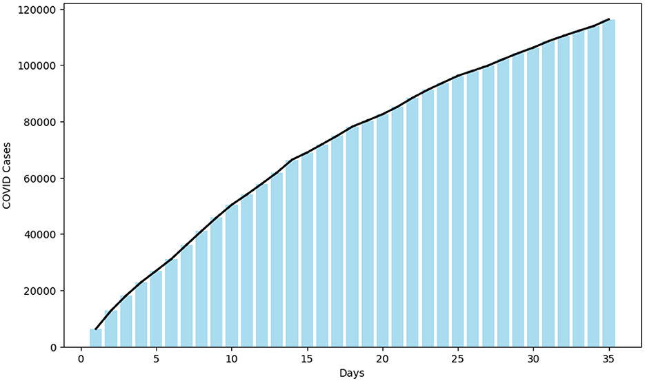
Figure 1. Daily cumulative COVID cases with slope lines.

Figure 2

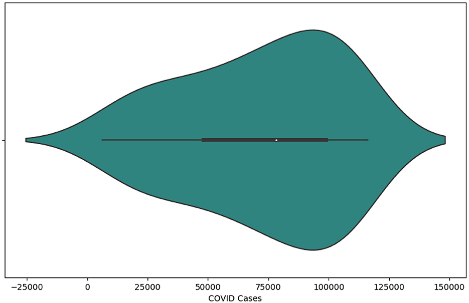
Figure 2. COVID cases distribution illustrated with violin plot.

The integrated violin and box plot depicted in Figure 2 offers a comprehensive visualization of the COVID data, presenting both the distribution characteristics and summary statistics within a unified representation. The white dot within the violin serves as a visual cue for the median, while the distinct central gray bar graphically represents the interquartile range. Adjacent to this bar, a subtle gray line extends to illustrate the broader data distribution. Kernel density estimations on either side of this central gray line delineate the shape of the data's distribution. The varying width of the violin dynamically conveys the density or frequency of data points, with a broader section indicating a higher concentration within the given range. The symmetry of the violin plot indicates the absence of skewness in the dataset.

Subsequently, we conduct a numerical modeling simulation utilizing authentic data to model the transference momentum of COVID-19 in Thailand. The approach involves the estimation of certain parameters, drawing from existing literature, while the remaining parameters are meticulously adjusted to enhance model accuracy. We fitted the COVID-19 Model (Equation 1) to the increasing cases of COVID-19 in Thailand. Specifically, we focus on the Daily Cumulative cases of COVID-19 spanning from May 19, 2022, to June 22, 2022, as reported by the World Health Organization (WHO).¹ The fitting of the model was executed utilizing the fmincon algorithm within the MATLAB environment. This integration of real-world data into our simulation not only bolsters the reliability of our model but also facilitates a more extensive comprehension of the COVID-19 transmission dynamics within the context of Thailand during the specified time.

In this study, we conducted numerical simulations to validate the outcomes of our proposed model, employing the Caputo fractional derivative and solvers implemented in the MATLAB programming language. The purpose of these simulations was to complement and validate the analytical results obtained. To provide a visual illustration, we chose baseline values of parameter (refer to Table 2) that align with the characteristics of COVID-19 contamination and transmission.

Table 2

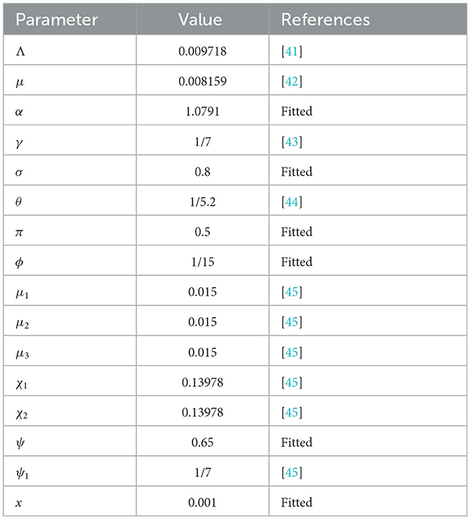
Table 2. Parameter values of model.

For data fitting, we gathered daily authenticated cases of COVID-19 in Thailand from May 19, 2022, to June 22, 2022, sourced from the World Health Organization (WHO), as outlined in Table 3. The results of the data fitting process are visually presented in Figure 3, utilizing the values derived from this dataset. The model was initialized with the initial conditions (Equation 3)

$\begin{array}{l}S(0)=7\times 10^7,E(0)=8\times 10^3,Q(0)=2\times 10^3,A(0)=3\times 10^2,\\ I(0)=5005,R(0)=0.\end{array}$

Table 3

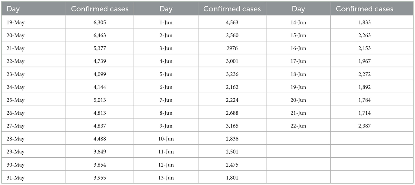
Table 3. The daily confirmed cases of COVID-19 in Thailand from May 19, 2022, to June 22, 2022.

Figure 3

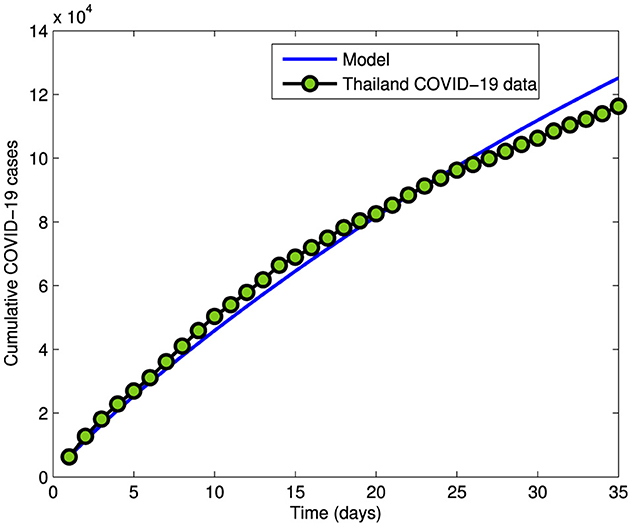
Figure 3. Daily cumulative cases of COVID-19 from May 19, 2022 to June 22, 2022.

Figure 4 displays the variations observed in the numerical simulation of Model (Equation 2), initialized with values specified in Equation 3 and utilizing parameter values from Table 2. The simulation involves varying the order of the fractional derivative, denoted as η, with values ranging from 0 to 1. Specifically, we explore the impact on the dynamics of S(t), A(t), I(t), Q(t), E(t), and R(t) over time. In this analysis, η is considered with discrete values of 0.4, 0.6, 0.8, and 1, allowing us to observe and analyze the resulting changes in the model's outputs.

Figure 4

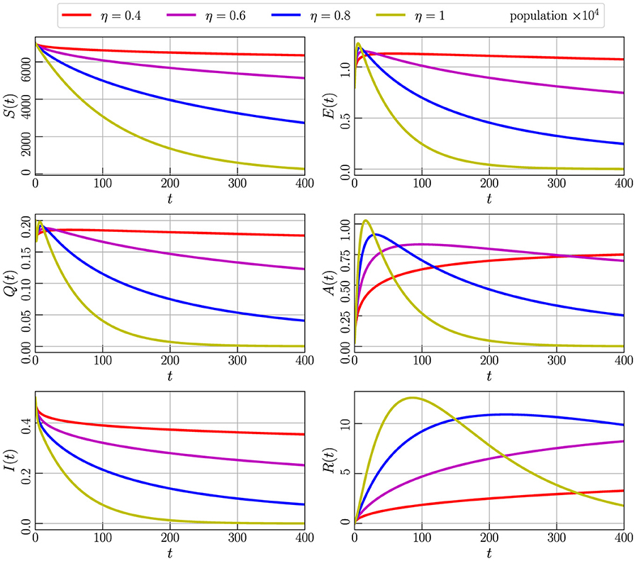
Figure 4. Numerical simulation of model (Equation 4) with initial values (Figure 3) using parameter values given by Table 2 and varying the order of the derivative η.

5.1.2 Impact of parameters

The importance of home remedies in influencing the spread rate of COVID-19 is crucial, particularly during times of quarantine. By employing a combination of precautionary measures and home remedies, individuals can observe a noticeable shift toward recovery. This section aims to demonstrate the impact of a specific parameter, denoted as ψ₁. Through the implementation of various levels of ψ₁, we can analyze and understand how these home-based interventions contribute to the overall trajectory of recovery. Home remedies, ranging from herbal infusions and nutritional supplements to respiratory exercises, not only bolster the immune system but also play a significant role in managing symptoms and reducing the severity of the illness. As we explore the effectiveness of different levels of ψ₁ in this context, it becomes evident that personalized and targeted home-based interventions can be instrumental in mitigating the transmission of the virus and expediting the recovery procedure for individuals affected by COVID-19.

In Figure 5, we represent the outcome of the numerical simulation of Model (Equation 2) with initial values specified in Equation 3, employing parameter values from Table 2, and setting α = 0.85 The simulation involves varying the parameter ψ₁, and we observe corresponding variations in all compartments. Specifically, we consider values for ψ₁ as 0.1, 0.2, 0.3, and 0.4. The graph illustrates that an increment in the ψ₁ parameter leads to a decline in the populations of compartments A, I, Q, and E, while the number of recovered individuals increases. Detailed numerical data supporting these observations can be found in Table 4. This graphical representation underscores the significance of the ψ₁ parameter in influencing the dynamics of the model and its impact on the various compartments.

Figure 5

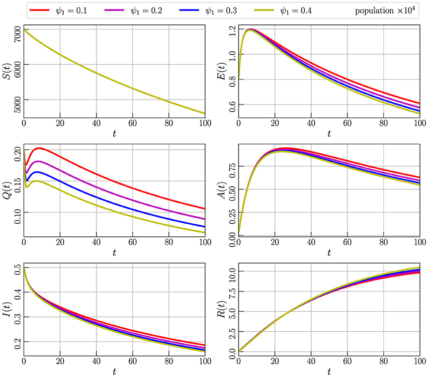
Figure 5. Numerical simulation of model (Equation 4) with initial values (Figure 3) using parameter values given by Table 2, α = 0.85, and varying the parameter ψ₁.

Table 4

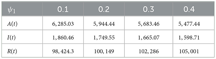
Table 4. Results of fractional model with various of ψ₁.

Figure 6 illustrates the outcome of the numerical simulation for Model (Equation 2) with initial values specified in Equation 3, utilizing parameter values from Table 2 and setting α to 0.85. The simulation involves varying the parameter γ, which represents the transmission of the population from E (exposed) to Q (quarantine). Specifically, we consider γ values of 0.1, 0.2, 0.3, and 0.4. It becomes evident from the graph that an increase in the γ parameter corresponds to a higher number of individuals transitioning to quarantine over time. This, in turn, leads to a decrease in the populations of symptomatic (A and I) and asymptomatic (E) compartments, while the number of cured people increases. The observed dynamics highlight the influence of the γ parameter on the distribution of individuals across different compartments and underscore its role in shaping the outcomes of the model.

Figure 6

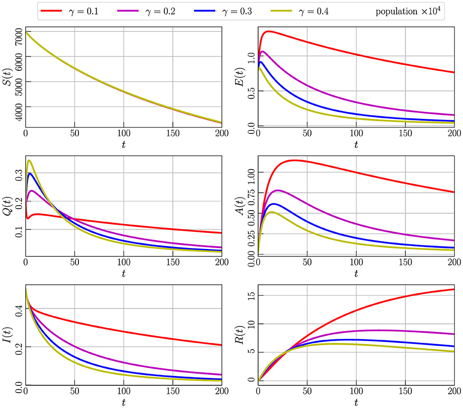
Figure 6. Numerical simulation of model (Equation 4) with initial values (Figure 3) using parameter values given by Table 2, α = 0.85, and varying the parameter γ.

Figure 7 depicts the numerical simulation outcome of Model (Equation 2) with initial values specified in Equation 3, utilizing parameter values from Table 2 and setting α to 0.85. The simulation involves varying the parameter ϕ, which shows the transmission rate of individuals from the quarantine compartment (Q) to the infected compartment (I). Specifically, we examine the impact of ϕ by assigning values of 0.01, 0.06, 0.11, and 0.16. The graphical representation indicates that a decrease in the transmission rate corresponds to a reduction in the compartments containing COVID-19 positive individuals over time. This observation suggests that maintaining a low value for the ϕ parameter is crucial for the stability of the system. The figure underscores the importance of carefully tuning this parameter to control the dynamics of the model and ensure its stability.

Figure 7

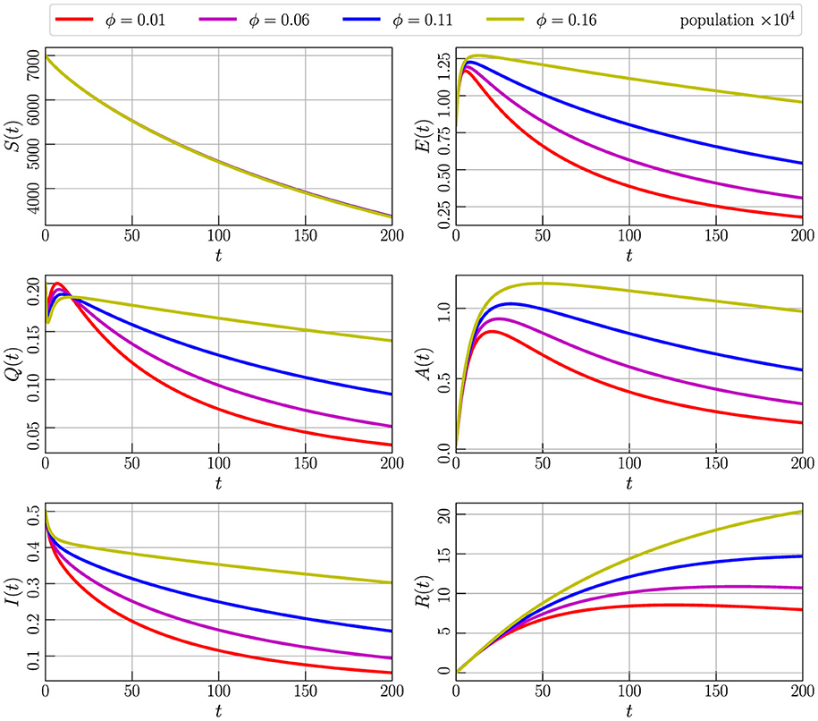
Figure 7. Numerical simulation of model (Equation 4) with initial values (Figure 3) using parameter values given by Table 2, α = 0.85, and varying the parameter ϕ.

In Figure 8, we present the results of numerical simulations for Model (Equation 2) with initial values specified in Equation 3, employing parameter values from Table 2 while setting α to 0.85. The simulations involve the variation of the parameter θ, representing the decease spreading rate of individuals from the exposed compartment (E) to the asymptomatic compartment (A). The graphs depict the behavior of the model as θ takes values of 0.1, 0.2, 0.3, and 0.4. Notably, an increase in θ leads to a corresponding increase in the population across all compartments. To maintain stability, it becomes apparent that a smaller value for θ is necessary. This observation emphasizes the critical role of parameter tuning, particularly for θ, in governing the stability of the model and influencing the dynamics within each compartment over time.

Figure 8

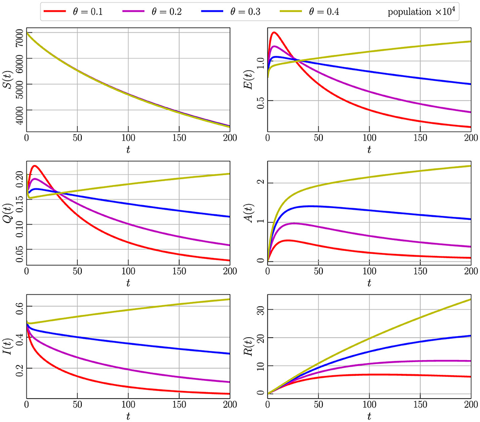
Figure 8. Numerical simulation of model (Equation 4) with initial values Figure 3 using parameter values given by Table 2, α = 0.85, and varying the parameter θ.

6 Conclusion

This study has investigated the intricate momentum of COVID-19 spreading by formulating a mathematical model that incorporates the integer fractional-order Caputo derivative. Our exploration encompassed crucial aspects such as identifying the region of feasibility, pinpointing equilibrium points, and calculating the fundamental reproduction number R₀. The application of fixed-point theory robustly established the existent of a unique solution to the model. Utilizing the Adams-Bashforth scheme, we derived approximate solutions for the system, allowing for a practical understanding of its behavior. Our simulations, based on real-world COVID-19 reports from Thailand, spanning from May 19, 2022, to June 22, 2022, provided valuable insights into equilibrium points and the reproduction number. Our findings confirm that the disease is anticipated to dwindle within the populace when the basic reproduction number is bounded by one, while persistence prevails when R₀ exceeds one. Moreover, our data analysis has deepened our understanding of disease transmission dynamics, offering a nuanced perspective on how COVID-19 behaves in the specific context of Thailand. Notably, our study sheds light on the impact of home remedies and precautionary measures on diminishing the disease and enhancing recovery rates, from Table 4, it is clear that home remedies influence the recovered individuals, as the value of ψ₁ increases from 0.1 to 0.4, causing individuals in compartments like A(t) and I(t) to decrease. This indicates how home remedies influence the rate of recovery even before individuals enter the asymptotically or symptomatically infected classes. In a similar vein, each graphical representation depicting the impact of a parameter provides a detailed insight into how that specific parameter influences the number of individuals involved in a given scenario. These representations serve as visual tools, offering a clear understanding of the dynamics at play within the system under consideration. By observing these graphs, we can discern the trends and patterns associated with the parameter's effect on the population dynamics. Furthermore, these graphical depictions offer valuable information on how we can effectively manage and control the spread of a certain phenomenon. By analyzing the trends illustrated in the graphs, we can identify strategies and interventions that prove effective in mitigating the spread of the phenomenon in question. Whether it involves adjusting certain parameters, implementing targeted interventions, or adopting preventive measures, these graphical representations serve as essential guides in devising strategies to curb the spread and maintain control over the situation. The comprehensive nature of our investigation not only contributes to the theoretical understanding of COVID-19 dynamics but also provides practical implications for managing and mitigating the impact of the pandemic. As we continue to navigate the complexities of the ongoing health crisis, these insights offer valuable guidance for public health strategies and individual actions in the pursuit of controlling and eventually overcoming the challenges posed by COVID-19.

Data availability statement

Publicly available datasets were analyzed in this study. This data can be found here: https://covid19.who.int/region/searo/country/th.

Author contributions

SE: Conceptualization, Data curation, Formal analysis, Investigation, Methodology, Resources, Software, Validation, Visualization, Writing – original draft, Writing – review & editing. SJ: Conceptualization, Data curation, Formal analysis, Investigation, Methodology, Project administration, Software, Supervision, Validation, Visualization, Writing – original draft, Writing – review & editing. HP: Data curation, Formal analysis, Investigation, Methodology, Resources, Software, Validation, Visualization, Writing – original draft, Writing – review & editing. AJ: Data curation, Formal analysis, Funding acquisition, Investigation, Project administration, Software, Supervision, Validation, Visualization, Writing – review & editing. BO: Data curation, Investigation, Methodology, Resources, Software, Validation, Visualization, Writing – review & editing. ZY: Formal analysis, Investigation, Methodology, Resources, Validation, Writing – review & editing.

Funding

The author(s) declare that no financial support was received for the research, authorship, and/or publication of this article.

Conflict of interest

The authors declare that the research was conducted in the absence of any commercial or financial relationships that could be construed as a potential conflict of interest.

Publisher's note

All claims expressed in this article are solely those of the authors and do not necessarily represent those of their affiliated organizations, or those of the publisher, the editors and the reviewers. Any product that may be evaluated in this article, or claim that may be made by its manufacturer, is not guaranteed or endorsed by the publisher.

Footnotes

1. ^https://covid19.who.int/region/searo/country/th

References

1. Jose SA, Raja R, Dianavinnarasi J, Baleanu D, Jirawattanapanit A. Mathematical modeling of chickenpox in Phuket: efficacy of precautionary measures and bifurcation analysis. Biomed Signal Proc Control. (2023) 84:104714. doi: 10.1016/j.bspc.2023.104714

Crossref Full Text | Google Scholar

2. Jose SA, Raja R, Omede BI, Agarwal RP, Alzabut J, Cao J, et al. Mathematical modeling on co-infection: transmission dynamics of Zika virus and Dengue fever. Nonlinear Dyn. (2023) 111:4879–914. doi: 10.1007/s11071-022-08063-5

Crossref Full Text | Google Scholar

3. Van den Driessche P, Watmough J. Reproduction numbers and sub-threshold endemic equilibria for compartmental models of disease transmission. Math Biosci. (2002) 180:29–48. doi: 10.1016/S0025-5564(02)00108-6

PubMed Abstract | Crossref Full Text | Google Scholar

4. Joseph D, Ramachandran R, Alzabut J, Jose SA, Khan H. A fractional-order density-dependent mathematical model to find the better strain of wolbachia. Symmetry. (2023) 15:845. doi: 10.3390/sym15040845

Crossref Full Text | Google Scholar

5. Jose SA, Ramachandran R, Baleanu D, Panigoro HS, Alzabut J, Balas VE. Computational dynamics of a fractional order substance addictions transfer model with Atangana-Baleanu-Caputo derivative. Math Methods Appl Sci. (2023) 46:5060–85. doi: 10.1002/mma.8818

Crossref Full Text | Google Scholar

6. Thomas R, Jose SA, Raja R, Alzabut J, Cao J, Balas VE. Modeling and analysis of SEIRS epidemic models using homotopy perturbation method: A special outlook to 2019-nCoV in India. Int J Biomathem. (2022) 15:2250059. doi: 10.1142/S1793524522500590

Crossref Full Text | Google Scholar

7. Jose SA, Ramachandran R, Cao J, Alzabut J, Niezabitowski M, Balas VE. Stability analysis and comparative study on different eco-epidemiological models: stage structure for prey and predator concerning impulsive control. Opt Control Applic Methods. (2022) 43:842–66. doi: 10.1002/oca.2856

Crossref Full Text | Google Scholar

8. Jose SA, Raja R, Zhu Q, Alzabut J, Niezabitowski M, Balas VE. Impact of strong determination and awareness on substance addictions: a mathematical modeling approach. Math Methods Appl Sci. (2022) 45:4140–60. doi: 10.1002/mma.7859

Crossref Full Text | Google Scholar

9. Haq F, Shah K, Rahman G, Shahzad M. Numerical analysis of fractional order model of HIV-1 infection of CD4+ T-cells. Comput Methods Differ Equ. (2017) 5:1–11.

Google Scholar

10. Koca I. Analysis of rubella disease model with non-local and non-singular fractional derivatives. Int J Optimiz Contr. (2018) 8:17–25. doi: 10.11121/ijocta.01.2018.00532

Crossref Full Text | Google Scholar

11. Rida SZ, Arafa AA, Gaber YA. Solution of the fractional epidemic model by L-ADM. J Fract Calc Appl. (2016) 7:189–95. doi: 10.21608/jfca.2016.308382

Crossref Full Text | Google Scholar

12. Akbari Kojabad E, Rezapour S. Approximate solutions of a sum-type fractional integro-differential equation by using Chebyshev and Legendre polynomials. Adv Differ Equat. (2017) 2017:1–8. doi: 10.1186/s13662-017-1404-y

Crossref Full Text | Google Scholar

13. Talaee M, Shabibi M, Gilani A, Rezapour S. On the existence of solutions for a pointwise defined multi-singular integro-differential equation with integral boundary condition. Adv Differ Equat. (2020) 2020:1–6. doi: 10.1186/s13662-020-2517-2

Crossref Full Text | Google Scholar

14. Qureshi S. Monotonically decreasing behavior of measles epidemic well captured by Atangana-Baleanu-Caputo fractional operator under real measles data of Pakistan. Chaos, Solit Fract. (2020) 131:109478. doi: 10.1016/j.chaos.2019.109478

Crossref Full Text | Google Scholar

15. Ali Dokuyucu M, Celik E, Bulut H, Mehmet Baskonus H. Cancer treatment model with the Caputo-Fabrizio fractional derivative. Eur Phys J Plus. (2018) 133:1–6. doi: 10.1140/epjp/i2018-11950-y

Crossref Full Text | Google Scholar

16. Jan R, Qureshi S, Boulaaras S, Pham VT, Hincal E, Guefaifia R. Optimization of the fractional-order parameter with the error analysis for human immunodeficiency virus under Caputo operator. Discr Contin Dyn Syst S. (2023) 16:2118–40. doi: 10.3934/dcdss.2023010

Crossref Full Text | Google Scholar

17. Jan R, Khan A, Boulaaras S, Ahmed Zubair S. Dynamical behaviour and chaotic phenomena of HIV infection through fractional calculus. Discr Dyn Nat Soc. (2022) 2022:5937420. doi: 10.1155/2022/5937420

Crossref Full Text | Google Scholar

18. Jan A, Boulaaras S, Abdullah FA, Jan R. Dynamical analysis, infections in plants, and preventive policies utilizing the theory of fractional calculus. Eur Phys J Special Topics. (2023) 232:2497–512. doi: 10.1140/epjs/s11734-023-00926-1

Crossref Full Text | Google Scholar

19. Alharbi R, Jan R, Alyobi S, Altayeb Y, Khan Z. Mathematical modeling and stability analysis of the dynamics of monkeypox via fractional-calculus. Fractals. (2022) 30:2240266. doi: 10.1142/S0218348X22402666

Crossref Full Text | Google Scholar

20. Lanbaran NM, Çelik E. Prediction of breast cancer through tolerance-based intuitionistic fuzzy-rough set feature selection and artificial neural network. Gazi University J Sci. (2021) 34:1064–1075. doi: 10.35378/gujs.857099

Crossref Full Text | Google Scholar

21. Dokuyucu M, Çelik E. Analyzing a novel coronavirus model (COVID-19) in the sense of Caputo-Fabrizio fractional operator. Appl Comput Mathem. (2021) 20:49–69.

Google Scholar

22. Shah Z, Bonyah E, Alzahrani E, Jan R, Aedh Alreshidi N. Chaotic phenomena and oscillations in dynamical behaviour of financial system via fractional calculus. Complexity. (2022) 2022:8113760. doi: 10.1155/2022/8113760

Crossref Full Text | Google Scholar

23. Jan R, Boulaaras S, Shah SA. Fractional-calculus analysis of human immunodeficiency virus and CD4+ T-cells with control interventions. Commun Theor Phys. (2022) 74:105001. doi: 10.1088/1572-9494/ac7e2b

Crossref Full Text | Google Scholar

24. Tang TQ, Jan R, Bonyah E, Shah Z, Alzahrani E. Qualitative analysis of the transmission dynamics of dengue with the effect of memory, reinfection, and vaccination. Comput Math Methods Med. (2022) 2022:7893570. doi: 10.1155/2022/7893570

PubMed Abstract | Crossref Full Text | Google Scholar

25. Jan A, Srivastava HM, Khan A, Mohammed PO, Jan R, Hamed YS. In vivo HIV dynamics, modeling the interaction of HIV and immune system via non-integer derivatives. Fract Fract. (2023) 7:361. doi: 10.3390/fractalfract7050361

Crossref Full Text | Google Scholar

26. Jan R, Razak NN, Boulaaras S, Rajagopal K, Khan Z, Almalki Y. Fractional perspective evaluation of chikungunya infection with saturated incidence functions. Alexandr Eng J. (2023) 83:35–42. doi: 10.1016/j.aej.2023.10.036

Crossref Full Text | Google Scholar

27. Jan R, Razak NN, Alyobi S, Khan Z, Hosseini K, Park C, et al. Fractional dynamics of chronic lymphocytic leukemia with the effect of chemoimmunotherapy treatment. Fractals. (2024) 15:2440012. doi: 10.1142/S0218348X24400127

Crossref Full Text | Google Scholar

28. Anggriani N, Panigoro HS, Rahmi E, Peter OJ, Jose SA. A predator-prey model with additive Allee effect and intraspecific competition on predator involving Atangana-Baleanu-Caputo derivative. Results in Physics. (2023) 49:106489. doi: 10.1016/j.rinp.2023.106489

Crossref Full Text | Google Scholar

29. Caputo M, Fabrizio M. A new definition of fractional derivative without singular kernel. Progr Fract Different Applic. (2015) 1:73–85. doi: 10.12785/pfda/010201

Crossref Full Text | Google Scholar

30. Singh R, Mishra J, Gupta VK. Dynamical analysis of a Tumor Growth model under the effect of fractal fractional Caputo-Fabrizio derivative. Int J Math Comput Eng. (2023) 1:115–26. doi: 10.2478/ijmce-2023-0009

Crossref Full Text | Google Scholar

31. Atangana A, Baleanu D. New fractional derivatives with nonlocal and non-singular kernel: theory and application to heat transfer model. Therm Sci. (2016) 20:763–9. doi: 10.2298/TSCI160111018A

Crossref Full Text | Google Scholar

32. Edward S, Raymond KE, Gabriel KT, Nestory F, Godfrey MG, Arbogast MP, et al. mathematical model for control and elimination of the transmission dynamics of measles. Appl Comput Mathem. (2015) 4:396–408. doi: 10.11648/j.acm.20150406.12

Crossref Full Text | Google Scholar

33. De la Sen M, Alonso-Quesada S, Ibeas A, Nistal R. On a discrete SEIR epidemic model with two-doses delayed feedback vaccination control on the susceptible. Vaccines. (2021) 9:398. doi: 10.3390/vaccines9040398

PubMed Abstract | Crossref Full Text | Google Scholar

34. Gomes MG, Ferreira MU, Corder RM, King JG, Souto-Maior C, Penha-Gonçalves C, et al. Individual variation in susceptibility or exposure to SARS-CoV-2 lowers the herd immunity threshold. J Theor Biol. (2022) 540:111063. doi: 10.1016/j.jtbi.2022.111063

PubMed Abstract | Crossref Full Text | Google Scholar

35. Annas S, Pratama MI, Rifandi M, Sanusi W, Side S. Stability analysis and numerical simulation of SEIR model for pandemic COVID-19 spread in Indonesia. Chaos, Solit Fract. (2020) 139:110072. doi: 10.1016/j.chaos.2020.110072

PubMed Abstract | Crossref Full Text | Google Scholar

36. Moore S, Hill EM, Tildesley MJ, Dyson L, Keeling MJ. Vaccination and non-pharmaceutical interventions for COVID-19: a mathematical modelling study. Lancet Infect Dis. (2021) 21:793–802. doi: 10.1016/S1473-3099(21)00143-2

PubMed Abstract | Crossref Full Text | Google Scholar

37. Yaagoub Z, Danane J, Allali K. On a two-strain epidemic mathematical model with vaccination. Comput Methods Biomech Biomed Engin. (2024) 27:632–50. doi: 10.1080/10255842.2023.2197542

PubMed Abstract | Crossref Full Text | Google Scholar

38. Diethelm K, Ford NJ, Freed AD. A predictor-corrector approach for the numerical solution of fractional differential equations. Nonlinear Dyn. (2002) 29:3–22. doi: 10.1023/A:1016592219341

Crossref Full Text | Google Scholar

39. Nishant BS, Purohit SD, Nisar KS, Munjam SR. Some fractional calculus findings associated with the product of incomplete ℵ-function and Srivastava polynomials. Int J Math Comput Eng. (2024) 2:97–116. doi: 10.2478/ijmce-2024-0008

Crossref Full Text | Google Scholar

40. Abdulazeez ST, Modanli M. Analytic solution of fractional order Pseudo-Hyperbolic Telegraph equation using modified double Laplace transform method. Int J Math Comput Eng. (2023) 1:105–14. doi: 10.2478/ijmce-2023-0008

Crossref Full Text | Google Scholar

41. Thailand Death Rate 1950–2024. Available online at: https://www.macrotrends.net/countries/THA/thailand/death-rate

Google Scholar

42. Thailand Birth Rate 1950–2024. Available online at: https://www.macrotrends.net/countries/THA/thailand/birth-rate

Google Scholar

43. Omede BI, Odionyenma UB, Ibrahim AA, Bolaji B. Third wave of COVID-19: mathematical model with optimal control strategy for reducing the disease burden in Nigeria. Int J Dyn Control. (2023) 11:411–27. doi: 10.1007/s40435-022-00982-w

PubMed Abstract | Crossref Full Text | Google Scholar

44. Rothan HA, Byrareddy SN. The epidemiology and pathogenesis of coronavirus disease (COVID-19) outbreak. J Autoimmun. (2020) 109:102433. doi: 10.1016/j.jaut.2020.102433

PubMed Abstract | Crossref Full Text | Google Scholar

45. Okuonghae D, Omame A. Analysis of a mathematical model for COVID-19 population dynamics in Lagos, Nigeria. Chaos, Solit Fract. (2020) 139:110032. doi: 10.1016/j.chaos.2020.110032

PubMed Abstract | Crossref Full Text | Google Scholar