Tuberculosis and COVID-19 co-infection is currently the major issue of public health in many nations, including Ghana. Therefore, to explore the effects of the two Tuberculosis strains on COVID-19, we suggest a Tuberculosis and COVID-19 co-infection model. The study also provides the most economical and effective control methods to reduce the co-infection of tuberculosis and COVID-19. Based on the behavioral patterns of the two Tuberculosis strains and COVID-19 reproduction numbers, the stability of the co-infection model is examined. We explore the sensitivity of the parameters to examine the effect of the drug-resistant and drug-sensitive strain of Tuberculosis on the co-infection of COVID-19. We determine the most cost-effective and optimal treatment strategies that aim to maximize outcomes while minimizing tuberculosis and/or COVID-19 incidences, cost-effectiveness, and optimization approaches. The outcomes of this work contribute to a better understanding of Tuberculosis and COVID-19 epidemiology and provide insights into implementing interventions needed to minimize Tuberculosis and COVID-19 burden in similar settings worldwide.

Introduction

Over time, tuberculosis (TB) has emerged as a major public health concern due to its spread, particularly in developing nations. This is because tuberculosis is endemic in these nations, where drug-resistant tuberculosis, poverty, and insufficient diagnostic techniques are some of the factors that make the disease more difficult to treat [1]. World Health Organization (WHO) health statistics from [2] account that ~1.4 million deaths were attributed to tuberculosis (TB) out of the 10.4 million cases reported globally in 2015 [3]. This indicates that tuberculosis (TB) affects about one-third of the world's population each year, which makes it one of the top 10 leading causes of death worldwide.

Due to vaccine inefficacy, chemotherapy has been the cornerstone of apparent control programs for TB. Antibiotic treatment for drug-resistant strains of TB patients is much more expensive and takes time compared with drug-sensitive strains of TB patients. Antibiotic-resistant tuberculosis (TB), which increases the risk of relapse and can arise from medication treatment non-compliance, is seriously harming public health and has become a societal problem [4, 5].

Conversely, COVID-19 caused over 6 million deaths globally, and approximately, by March 2022, 480 million incidences were reported. Presently, there is growing evidence that patients with drug-sensitive TB and drug-resistant TB disease are more likely to develop a severe case of COVID-19, as reported in [6]. Even in cases where the force of reinfection is relatively weak, the COVID-19 reinfection scenario using the SIR model demonstrates that transmission could arise as a result of the immunity waning [7]. A COVID-19 model, which involves infection via items induced with SARS-CoV-2, is proposed to be made public aware [8]. The disease COVID-19 spreads swiftly, sparking a pandemic and posing a threat to world health. Other sectors, particularly the socioeconomic sector, have been significantly impacted by the pandemic [9]. According to the World Meter, as of 30 April 2022, there were 6,257,512 COVID-19 fatalities worldwide and 512,466,045 reported incidences. The results emphasize the necessity of taking steps to minimize the transmission of COVID-19 and TB. One way mathematics is essential to simulating the disease's epidemic phenomenon is by using a deterministic model to study the disease's transmission. Numerous developments have been made in analyzing the COVID-19 model with declining immunity. The natural immunity period is for the latter group, and models with symptomatic and asymptomatic infected populations show that the vaccine efficacy level determines when to begin the massive vaccination strategy [10].

The respiratory disease known as Coronavirus Disease 2019 (COVID-19) is a member of the Coronaviridae family. The α-Coronavirus, β-Coronavirus, γ-Coronavirus, and δ-Coronavirus are the four strain varieties of the virus. Humans are impacted by the first two, but bird infections are the main cause of the remaining two [11]. The source and origin of the virus are still unknown, despite the fact that COVID-19 is classified as a zoonotic disease and linked to the family of bats. After SARS and MERS, COVID-19 is the third new coronavirus of the 21st century to generate a significant outbreak that swept across 210 countries globally [12]. The variations of concern (VOC) introduce additional uncertainties and hamper efforts to prevent the disease, even as promising new vaccinations have emerged. VOCs, as described by the US Centers for Disease Control and Prevention, are more severe and highly transmissible strains of SARS-CoV-2 that significantly reduce vaccine effectiveness. Since December 2020, a number of VOCs have surfaced. Not long after the β-Coronavirus variation (B.1.351) was reported in South Africa, the α-Coronavirus variant (B.1.1.7) was initially identified with a 50% higher transmission in the United Kingdom. The δ-Coronavirus version (B.1.167.2) was originally discovered in India and classified on 11th May 2021 [13], whereas the γ-Coronavirus variant (P.1) was initially discovered in Brazil [14].

While less severe than earlier VOCs, the Omicron variety (B.1.1.529) is even more transmissible than δ-Coronavirus and was first discovered in South Africa and Botswana in 2021 [15]. Large recent increases in new COVID cases across national boundaries have been attributed to these variations. Countries with high vaccination rates experienced notable increases in incidence when the δ-Coronavirus variety emerged as the predominant virus worldwide [16]. Vaccines are less efficient in preventing δ-Coronavirus than previous forms, which made it more deadly. One dose of BNT162b2 (Pfizer-BioNTech) or ChAdOx1 (AstraZeneca) provides immunity against the δ-Coronavirus VOC, although immunity against the α-Coronavirus VOC is 45–52% [16]. Less protection against the δ-Coronavirus form was also demonstrated to be conferred by receiving two doses [16]. The enormous increases in infectious cases we saw globally in 2021 were caused by a lower mutation in the receptor-binding region of the δ-Coronavirus SARS-CoV-2 spike protein [17]. The Omicron version caused much greater worldwide spikes in cases in December 2021. Compared to the wild-type strain, Omicron was discovered to contain 33 mutations in its spike protein [18]. Given that vaccines lose their effectiveness over time and society reopens to more viral encounters, countries must reevaluate how best to implement vaccination programs in light of the significant changes that have been observed across a variety of volatile organic compounds.

While the World Health Organization and the Centers for Disease Control and Prevention have released certain health advisories and suggestions for individuals who are more susceptible to negative results from COVID-19, individuals who are co-infected with COVID-19 and have TB are at higher risk of dying [19]. A number of studies have suggested that COVID-19 may exacerbate or reactivate tuberculosis (TB), and some have even linked tuberculosis to severe COVID-19 [20–22]. Pathology-wise, diseases caused by SARS-CoV-2 and Mycobacterium tuberculosis to the immunomodulation tend to cause an imbalanced inflammatory response, which furthers the development and deterioration of both diseases [23]. In addition, patients with severe COVID-19 may be more susceptible to reactivation or new infection-related active TB [24].

The aforementioned issues motivate this study to explore the optimal control strategies incorporating cost-effectiveness analysis to mitigate TB and COVID-19. The next section illustrates the co-infection model assumptions and formulation such that people with latent TB will become active at a specific rate. Additionally, it assumes that some treated patients with active tuberculosis will not complete their course of treatment and that some of them will develop drug-resistant tuberculosis. Four control mechanisms for public education, vaccination, case finding, and case holding efforts are incorporated into this model. The article is arranged as follows: Section 2 presents the detailed framework of the epidemiological co-infection model, together with the definition of the parameters and respective values. Section 3 presents the analysis of the model's positivity of solutions, computation of the sub-models' reproduction numbers, and stability of the sub-models. Section 4 presents the model parameters estimation and sensitivity. Section 5 presents the optimal control analysis. Section 6 presents the cost-effectiveness analysis. Finally, Section 7 presents the concluding remarks of this study.

The tuberculosis (TB) and COVID-19 model

The proposed epidemiological model comprising tuberculosis and COVID-19 vaccination is characterized by two sub-models (TB and COVID-19) with the following features. It is divided into 12 distinct compartments, namely S(t): Susceptible class, V(t): Vaccinated class, E_st(t): individuals exposed to drug-sensitive (DS) strain TB only, I_st(t): Individuals infectious with drug-sensitive (DS) TB only, E_rt(t): Individuals exposed to drug-resistant (DR) strain of TB only, I_rt(t): Individuals infectious with drug-resistant (DR) strain TB only, E_c(t): COVID-19 exposed individuals only, I_c(t): Individuals infectious with COVID-19 only, I_stc(t): Individuals infectious with drug-sensitive (DS) strain of TB and COVID-19, I_rtc(t): Individuals infectious with drug-resistant (DR) strain of TB and COVID-19, T(t): Treated class consisting of individuals from both strains of TB, and R(t): Recovered class consisting of treated individuals of TB and/or COVID-19. The dynamics of the model are as follows:

• We illustrate the TB stream of the model; susceptible and vaccinated individuals are exposed to either a drug-sensitive (DS) strain or drug-resistant (DR) strain of tuberculosis where S(t) compartment recruit individuals by Λ, where individuals in S(t) and V(t) are infected by the two strains at the rate of β_stSI_st, β_rtSI_rt and σβ_stVI_st, σβ_rtVI_rt respectively, where σ belonging to [0, 1] denotes the vaccine protection rate. If σ = 0, then the vaccination protection is 100% efficient, σ = 1 implies that the vaccination protection efficiency is 0 and the immunity waning rate coefficient in the vaccinated host is ϑ, which is given as ϑ ≥ 1. We assume that a proportion of b and 1 − b of the individuals in S(t) enters the drug-sensitive (DS) classes I_st(t) and E_st(t), respectively, and a proportion of b and (1 − b) of the individuals in V(t) enter I_st(t) and E_st(t), respectively, similar to the drug-resistant (DR) classes by I_rt(t) and E_rt(t), where the rate of death due to drug-sensitive (DS) strain of TB disease is given as d₁ and the rate of death due to drug-resistant (DR) strain of TB disease is given as d₂. Here, we assume that induced TB death rates are different for drug-sensitive (DS) and drug-resistant (DR) strains of TB due to differences in transmission rate and response to prophylaxis. The individuals in E_st(t) identified to be infected move to T(t) at the rate of γ₁ for prophylaxis while the rest move to I_st(t) at the rate of δ_st. Individuals in E_rt(t) moves to I_rt(t) at the rate of δ_rt. A proportion of k I_st(t) individuals move to I_stc(t) at the rate of kγ₂ due to COVID-19 infection at the same time, while a proportion of 1 − k moves to T(t) at the rate of (1 − k)γ₂ for prophylaxis. Again, a proportion of m individuals in I_rt(t) move to I_rtc(t) at the rate of mγ₃ due to COVID-19 infection at the same time, while a proportion of 1 − m moves to T(t) at the rate of (1 − m)γ₃ for prophylaxis, where k, m belong to [0, 1]. The individuals in T(t) compartment who undergo successful prophylaxis recover at the rate of ε₅ while the rest are re-infected by ωλ₁, where ω = [0, 1] due to unsuccessful prophylaxis.

• We illustrate the COVID-19 stream of the model; susceptible and vaccinated individuals are exposed to COVID-19 at the rate of β_cSI_c and σβ_cVI_c, respectively. The individuals in E_c(t) identified with mild symptoms of the disease can recover at the rate of ε₁ due to strong immunity, while the rest become infected and move to I_c(t) at the rate of δ_c. The individuals in I_c(t) recover at the rate of ε₂, while others may develop any strains of TB and move to I_stc(t), I_rtc(t) at the rate of φ₁, φ₂, respectively. A proportion of g I_st(t) individuals move to I_st(t) at the rate of gε₃, while a proportion of (1 − g) recovers at the rate of (1 − g)ε₃; similarly, individuals in I_rtc(t) move to I_rt(t) at the rate of hε₄, while a proportion of 1 − h recovers at the rate of (1 − h)ε₄ where g, h belong to [0, 1). The respective rate of death due to TB and/or COVID-19 infection is given as d_i, where i = 3, 4, 5 respectively. The meanings of the rest of the parameters illustrated in the model are tabulated. The control efforts U₁(t), U₂(t), U₃(t), and U₄(t) for optimal control analysis would be applied and explained in detail in the subsequent section.

The total population N(t) in Equation (1) is defined based on the flowchart diagram Figure 1 as follows:

$\begin{array}{c}N(t)=S(t)+V(t)+E_{st}(t)+I_{st}(t)+E_{rt}(t)+I_{rt}(t)+\\ E_c(t)+I_c(t)+I_{stc}(t)+I_{rtc}(t)+T(t)+R(t).& (1)\end{array}$

Figure 1

Figure 1. Flowchart representation of the TB-COVID-19 vaccination model.

We formulate the model [see Equation (2)] as follows:

$\begin{array}{ll}\{\begin{array}{c}\frac{dS}{dt}=\Lambda +\vartheta V-(1-b){\lambda }_{1}S-a_{1}S,\\ \frac{dV}{dt}=\alpha S-(1-b){\lambda }_1\sigma V-a_{2}V,\\ \frac{d{E}_{st}}{dt}=\frac{\left[(1-b)(S+\sigma V)+b\omega T\right]{\beta }_{st}{I}_{st}}{N}-a_3{E}_{st},\\ \frac{d{I}_{st}}{dt}=\frac{\left[b(S+\sigma V)+(1-b)\omega T\right]{\beta }_{st}{I}_{st}}{N}+{\delta }_{st}{E}_{st}+g{\epsilon }_3{I}_{stc}-a_4{I}_{st},\\ \frac{d{E}_{rt}}{dt}=\frac{\left[(1-b)(S+\sigma V)+b\omega T\right]{\beta }_{rt}{I}_{rt}}{N}-a_5{E}_{rt},\\ \frac{d{I}_{rt}}{dt}=\frac{\left[b(S+\sigma V)+(1-b)\omega T\right]{\beta }_{rt}{I}_{rt}}{N}+{\delta }_{rt}{E}_{rt}+h{\epsilon }_3{I}_{rtc}-a_6{I}_{rt},\\ \frac{d{E}_c}{dt}=\frac{(S+\sigma V){\beta }_c{I}_c}{N}-a_7{E}_c,\\ \frac{d{I}_c}{dt}={\delta }_c{E}_c-a_8{I}_c,\\ \frac{d{I}_{stc}}{dt}={\phi }_1{I}_c+k{\gamma }_2{I}_{st}-a_9{I}_{stc},\\ \frac{d{I}_{rtc}}{dt}={\phi }_2{I}_c+m{\gamma }_3{I}_{rt}-a_{10}{I}_{rtc},\\ \frac{dT}{dt}={\gamma }_1{E}_{st}+(1-k){\gamma }_2{I}_{st}+(1-m){\gamma }_3{I}_{rt}-(\mu +{\epsilon }_5+\omega {\lambda }_1)T,\\ \frac{dR}{dt}={\epsilon }_1{E}_c+{\epsilon }_2{I}_c+(1-g){\epsilon }_3{I}_{stc}+(1-h){\epsilon }_4{I}_{rtc}+{\epsilon }_{5}T-\mu R.\end{array}& (2)\end{array}$

where ${\lambda }_1=\frac{\left[{\beta }_{st}{I}_{st}+{\beta }_{rt}{I}_{rt}\right]+{\beta }_c\left[I_c+I_{stc}+I_{rtc}\right]}{N},$ $a_1=\mu +\alpha ,$ $a_2=\mu +\vartheta ,$ $a_3=\mu +{\delta }_{st}+{\gamma }_1,$ $a_4=\mu +d_1+{\gamma }_2,$ $a_5=\mu +{\delta }_{rt},$ $a_6=\mu +d_2+{\gamma }_3,$ $a_7=\mu +{\delta }_c+{\epsilon }_1,$ $a_8=\mu +d_3+{\phi }_1+{\phi }_2+{\epsilon }_2,$ $a_9=\mu +d_4+{\epsilon }_3,$ $a_{10}=\mu +d_5+{\epsilon }_4.$

With initial conditions, S(0) ≥ 0, V(0) ≥ 0, E_st(0) ≥ 0, I_st(0) ≥ 0, E_rt(0) ≥ 0, I_rt(0) ≥ 0, E_c(0) ≥ 0, I_c(0) ≥ 0, I_stc(0) ≥ 0, I_rtc(0) ≥ 0, T(0) ≥ 0, R(0) ≥ 0. All the parameters of system (2) are non-negative.

TB and COVID-19 co-infection model's positivity and boundedness

The model (2) variables and parameters are non-negative since it is based on the population with TB and COVID-19. We state the following theorems to show that all variables of model (2) are non-negative and bounded.

Theorem 1: Define Y(t) = S(t), V(t), E_st(t), I_st(t), E_rt(t), I_rt(t), E_c(t), I_c(t), I_stc(t)I_rtc(t), T(t), R(t), if Y(0) ≥ 0, then Y(t) ≥ 0, and its solutions and initial values are non-negative for t > 0.

Proof: Let us consider the following instance that there exists an initial time t_i, such that

min{Y(t_i)} > 0 and min{Y(t)} > 0 for all t ∈ [0, t_i).

Here, Y(t) = S(t), V(t), E_st(t), I_st(t), E_rt(t), I_rt(t), E_c(t), I_c(t), I_stc(t)I_rtc(t), T(t), R(t). Without loss of generalization, min{Y(t_i)} = S(t_i).

Therefore, S(t_i) = 0, V(t_i) > 0 and S(t) > 0 for all t ∈ [0, t_i). However,

$\frac{dS(t_i)}{dt}=\Lambda +\vartheta V(t_i)>0,$

Since Λ ≥ 0, S(t_i)>S(0) ≥ 0.

This contradicts the claim S(t_i) = 0. Therefore, S(t)>0 for all t ≥ 0. This shows that all solutions are positive for t ≥ 0 in all other cases.

Theorem 2: To show the boundedness of solutions of model (2), define a positive invariant set as $Q=\left\{(S,V,E_{st},I_{st},E_{rt},I_{rt},E_c,I_c,I_{stc},I_{rtc},T,R)\in R_{+}^{12}:N(t)\le \frac{\Lambda }{\mu }\right\},$ which have positive solutions.

Proof: Let us consider the total population of model (2) N(t) as

$\begin{array}{c}N(t)=S(t)+V(t)+E_{st}(t)+I_{st}(t)+E_{rt}(t)+I_{rt}(t)+\\ E_c(t)+I_c(t)+I_{stc}(t)+I_{rtc}(t)+T(t)+R(t).& (3)\end{array}$

The rate of change of N(t) of Equation (3) is given as

$\begin{array}{c}{N}^{\prime }(t)=S^{\prime }(t)+V^{\prime }(t)+E_{st}^{\prime }(t)+I_{st}^{\prime }+\\ E_{rt}^{\prime }+I_{rt}^{\prime }+E_c^{\prime }+I_c^{\prime }+I_{stc}^{\prime }+I_{rtc}^{\prime }+T^{\prime }(t)+R^{\prime }(t),\\ N^{\prime }(t)=\Lambda -\mu S-\mu V-\mu E_{st}-(\mu +d_1)I_{st}-\mu E_{rt}-\\ (\mu +d_2)I_{rt}-\mu E_c-(\mu +d_3)I_c-\\ (\mu +d_4)I_{stc}-(\mu +d_5)I_{rtc}-\mu T-\mu R,\\ N^{\prime }(t)=\Lambda -\mu N(t)-(d_1{I}_{st}+d_2{I}_{rt}+d_3{I}_c+d_4{I}_{stc}+d_5{I}_{rtc})\\ \le \Lambda -\mu N(t).& (4)\end{array}$

This follows that from Equation (4),

$N(t)\le \frac{\Lambda }{\mu }(1-e^{-\mu t})+N(0)e^{-\mu t}.$

Then, $0<N(t)\le \frac{\Lambda }{\mu },$ if $N(0)\le \frac{\Lambda }{\mu }.$ That is, N(t) is bounded, and all solutions in Q approach enter or remain in Q. If t → ∞, 0 ≤ N(t) shows that N(t) is a set of positive invariant in the region $R_{+}^{12}.$ Therefore, the proof is complete.

Sub-models analysis

This subsection explores the reproduction numbers and the stability of the two sub-models.

Tuberculosis (TB) sub-model

The TB sub-model's disease-free equilibrium point is achieved by setting E_c = I_c = I_stc = I_rtc = R = 0 of system (2) and equate it to zero, the result in Equation (5) is as follows.

$\begin{array}{cc}\{\begin{array}{c}\frac{dS}{dt}=\Lambda +\vartheta V-\frac{(1-b)({\beta }_{st}{I}_{st}+{\beta }_{rt}{I}_{rt})S}{N}-a_{1}S,\\ \frac{dV}{dt}=\alpha S-\frac{(1-b)({\beta }_{st}{I}_{st}+{\beta }_{rt}{I}_{rt})\sigma V}{N}-a_{2}V,\\ \frac{d{E}_{st}}{dt}=\frac{\left[(1-b)(S+\sigma V)+b\omega T\right]{\beta }_{st}{I}_{st}}{N}-a_3{E}_{st},\\ \frac{d{I}_{st}}{dt}=\frac{\left[b(S+\sigma V)+(1-b)\omega T\right]{\beta }_{st}{I}_{st}}{N}+{\delta }_{st}{E}_{st}-a_4{I}_{st},\\ \frac{d{E}_{rt}}{dt}=\frac{\left[(1-b)(S+\sigma V)+b\omega T\right]{\beta }_{rt}{I}_{rt}}{N}-a_5{E}_{rt},\\ \frac{d{I}_{rt}}{dt}=\frac{\left[b(S+\sigma V)+(1-b)\omega T\right]{\beta }_{rt}{I}_{rt}}{N}+{\delta }_{rt}{E}_{rt}-a_6{I}_{rt},\\ \frac{dT}{dt}={\gamma }_1{E}_{st}+(1-k){\gamma }_2{I}_{st}+(1-m){\gamma }_3{I}_{rt}-\\ \left({\epsilon }_5+\frac{\omega (1-b)({\beta }_{st}{I}_{st}+{\beta }_{rt}{I}_{rt})}{N}\right)T.\end{array}& (5)\end{array}$

where N = S + V + E_st + I_st + E_rt + I_rt + T.

The TB sub-model (5) has a positive invariant in the region $R_{+}^7$ with $Q_T=\left\{(S,V,E_{st},I_{st},E_{rt},I_{rt},T)\in R_{+}^7:N(t)\le \frac{\Lambda }{\mu }\right\}$, as shown in Theorems 2 and 3.

Tuberculosis (TB) sub-model's basic reproduction number

Here, we define the basic reproduction number and the stability of the TB sub-model.

The disease-free equilibrium E_0T

It is globally stable, as demonstrated under the COVID-19 sub-model. The disease-free equilibrium E_0T = (S₀, V₀, 0, 0, 0, 0, 0) and the result is given in Equation (6).

$\begin{array}{c}{S}_0=\frac{\Lambda a_2}{a_1{a}_2-\vartheta \alpha },V_0=\frac{\Lambda \alpha }{a_1{a}_2-\vartheta \alpha },\\ E_{0T}=\left(\frac{\Lambda a_2}{a_1{a}_2-\vartheta \alpha },\frac{\Lambda \alpha }{a_1{a}_2-\vartheta \alpha },0,0,0,0,0\right).& (6)\end{array}$

The corresponding Jacobian matrix evaluated at disease-free equilibrium, J_E0T is given in Equation (7)

$\begin{array}{l}{J}_{E_{0T}}=\\ \left(\begin{array}{ccccccc}-a_1& \vartheta & 0& -\frac{(1-b){\beta }_{st}{S}_0}{N_0}& 0& -\frac{(1-b){\beta }_{rt}{S}_0}{N_0}& 0\\ \alpha & -a_2& 0& -\frac{(1-b){\beta }_{st}\sigma V_0}{N_0}& 0& -\frac{(1-b){\beta }_{rt}\sigma V_0}{N_0}& 0\\ 0& 0& -a_3& \frac{{(1-b)\beta }_{st}\left[S_0+\sigma V_0\right]}{N_0}& 0& 0& 0\\ 0& 0& {\delta }_{st}& \frac{b{\beta }_{st}\left[S_0+\sigma V_0\right]}{N_0}-a_4& 0& 0& 0\\ 0& 0& 0& 0& -a_5& \frac{(1-b){\beta }_{rt}\left[S_0+\sigma V_0\right]}{N_0}& 0\\ 0& 0& 0& 0& {\delta }_{rt}& \frac{b{\beta }_{rt}\left[S_0+\sigma V_0\right]}{N_0}-a_6& 0\\ 0& 0& {\gamma }_1& (1-k){\gamma }_2& 0& (1-m){\gamma }_3& -(\mu +{\epsilon }_5)\end{array}\right).& (7)\end{array}$

where N₀ = S₀ + σV₀ using the Jacobian at the disease-free equilibrium E_0T.

According to the explanation in [25], the spectral radius of the next-generation operator G = FV⁻¹ denotes the basic reproduction number. For sub-model (5), we have the square matrix with matrix F as the new infections and matrix V as the transition elements of the infected classes.

$\begin{array}{l}F=\left(\begin{array}{cccc}0& \frac{{(1-b)\beta }_{st}\left[S_0+\sigma V_0\right]}{N_0}& 0& 0\\ 0& \frac{b{\beta }_{st}\left[S_0+\sigma V_0\right]}{N_0}& 0& 0\\ 0& 0& 0& \frac{(1-b){\beta }_{rt}\left[S_0+\sigma V_0\right]}{N_0}\\ 0& 0& 0& \frac{b{\beta }_{rt}\left[S_0+\sigma V_0\right]}{N_0}\end{array}\right),\\ V=\left(\begin{array}{cccc}{a}_3& 0& 0& 0\\ -{\delta }_{st}& a_4& 0& 0\\ 0& 0& a_5& 0\\ 0& 0& -{\delta }_{rt}& a_6\end{array}\right).\end{array}$

Hence, the reproduction numbers are

$\begin{array}{l}{R}_{st}=\frac{{\left(1-b\right)\beta }_{st}{\delta }_{st}\left[S_0+\sigma V_0\right]}{N_0{a}_3{a}_4},R_{rt}=\frac{{\left(1-b\right)\beta }_{rt}{\delta }_{rt}\left[S_0+\sigma V_0\right]}{N_0{a}_5{a}_6},\end{array}$

where R_st and R_rt are the basic reproduction numbers of drug-sensitive (DS) and drug-resistant (DR) strains of TB, respectively. Substituting N₀, S₀ and V₀ give the following results:

$\begin{array}{l}{R}_{st}=\frac{{(1-b)\beta }_{st}{\delta }_{st}}{(\mu +{\delta }_{st}+{\gamma }_1)(\mu +d_1+{\gamma }_2)},\\ R_{rt}=\frac{{(1-b)\beta }_{rt}{\delta }_{rt}}{(\mu +{\delta }_{rt})(\mu +d_2+{\gamma }_3)},\end{array}$

The basic reproduction number is given as [see Equation (8)]

$\begin{array}{cc}{R}_{0T}=max\left\{R_{st},R_{rt}\right\}.& (8)\end{array}$

Existence of TB sub-model endemic equilibrium

We explore the existence and uniqueness of the endemic equilibrium of sub-model (5).

If R_rt > 1, then the drug-resistant (DR) strain has the dominance in sub-model (5) with $F_{rt}^{*}$ = $(S_{rt}^{*},V_{rt}^{*},0,0,E_{rt}^{*},I_{rt}^{*},T_{rt}^{*})$ as a unique endemic equilibrium for the drug-resistant (DR) strain. Then, the endemic equilibrium follows as

$\begin{array}{cc}\{\begin{array}{c}\Lambda +\vartheta V_{rt}^{*}-{\lambda }_1^{*}{S}_{rt}^{*}-a_1{S}_{rt}^{*}=0,\\ \alpha S_{rt}^{*}-{\lambda }_1^{*}\sigma V_{rt}^{*}-a_2{V}_{rt}^{*}=0,\\ \frac{\left[(1-b)(S_{rt}^{*}+\sigma V_{rt}^{*})+b\omega T_{rt}^{*}\right]{\beta }_{rt}{I}_{rt}^{*}}{N_{rt}^{*}}-a_5{E}_{rt}^{*}=0,\\ \frac{\left[b(S_{rt}^{*}+\sigma V_{rt}^{*})+(1-b)\omega T_{rt}^{*}\right]{\beta }_{rt}{I}_{rt}^{*}}{N_{rt}^{*}}+{\delta }_{rt}{E}_{rt}^{*}-a_6{I}_{rt}^{*}=0,\\ (1-m){\gamma }_3{I}_{rt}^{*}-({\epsilon }_5+\omega {\lambda }_1^{*})T_{rt}^{*}=0.\end{array}& (9)\end{array}$

where ${\lambda }_1^{*}=\frac{{(1-b)\beta }_{rt}{I}_{rt}^{*}}{N_{rt}^{*}}$ and $N_{rt}^{*}=S_{rt}^{*}+V_{rt}^{*}+E_{rt}^{*}+I_{rt}^{*}+T_{rt}^{*}.$

Simplifying Equation (9) gives the following.

$\begin{array}{cc}\{\begin{array}{c}{S}_{rt}^{*}=\frac{(a_2+\sigma {\lambda }_1^{*})\Lambda }{(a_1+{\lambda }_1^{*})(a_2+\sigma {\lambda }_1^{*})-\alpha \vartheta },\\ V_{rt}^{*}=\frac{\Lambda \alpha }{(a_1+{\lambda }_1^{*})(a_2+\sigma {\lambda }_1^{*})-\alpha \vartheta },\\ E_{rt}^{*}=\left[\frac{1}{a_5}\right]\left[\frac{{\lambda }_1^{*}\Lambda (a_2+\sigma {\lambda }_1^{*}+\sigma \alpha )}{(a_1+{\lambda }_1^{*})(a_2+\sigma {\lambda }_1^{*})-\alpha \vartheta }+\frac{b\omega {\beta }_{rt}(1-m){\gamma }_3{I}_{rt}^{*}}{({\epsilon }_5+\omega {\lambda }_1^{*})}\right],\\ T_{rt}^{*}=\frac{(1-m){\gamma }_3{I}_{rt}^{*}}{({\epsilon }_5+\omega {\lambda }_1^{*})}.\end{array}& (10)\end{array}$

Simplifying Equation (10) gives the following equation for $I_{rt}^{*}$.

$\begin{array}{c}{I}_{rt}^{*}=\left(\frac{\left({\epsilon }_5+\omega {\lambda }_1^{*}\right)\left(b\left(S_{rt}^{*}+\sigma V_{rt}^{*}\right)+a_5\right)}{{\beta }_{rt}^2{\delta }_{rt}\omega \left(1-m\right){\gamma }_3}\right)\left(\frac{\left(1-b\right){\beta }_{rt}{\delta }_{rt}}{a_5{a}_6}-1\right),\\ I_{rt}^{*}=\left(\frac{\left({\epsilon }_5+\omega {\lambda }_1^{*}\right)\left(\frac{b\Lambda \left(a_2+\sigma {\lambda }_2^{*}+\sigma \alpha \right)}{\left(a_1+{\lambda }_2^{*}\right)\left(a_2+\sigma {\lambda }_2^{*}\right)-\alpha \vartheta }+a_5\right)}{{\beta }_{rt}^2{\delta }_{rt}\omega \left(1-m\right){\gamma }_3}\right)\left(R_{rt}-1\right).& (11)\end{array}$

Since all the parameters associated with the model are non-negative, then from Equation (11) $I_{rt}^{*}$ is always positive if and only if R_rt > 1. Hence, there exist endemic equilibrium if R_rt > 1.

Again, if R_st > 1, then the drug-sensitive (DS) strain has the dominance in sub-model (5) with $F_{st}^{*}=(S_{st}^{*},V_{st}^{*},E_{st}^{*},I_{st}^{*},0,0,T_{st}^{*})$ as a unique endemic equilibrium of the drug-sensitive (DS) strain. Then, the endemic equilibrium follows as

$\begin{array}{cc}\{\begin{array}{c}\Lambda +\vartheta V_{st}^{*}-{\lambda }_2^{*}{S}_{st}^{*}-a_1{S}_{st}^{*}=0,\\ \alpha S_{st}^{*}-{\lambda }_2^{*}\sigma V_{st}^{*}-a_2{V}_{st}^{*}=0,\\ \frac{\left[(1-b)(S_{st}^{*}+\sigma V_{st}^{*})+b\omega T_{st}^{*}\right]{\beta }_{st}{I}_{st}^{*}}{N_{st}^{*}}-a_3{E}_{st}^{*}=0,\\ \frac{\left[b(S_{st}^{*}+\sigma V_{st}^{*})+(1-b)\omega T_{st}^{*}\right]{\beta }_{st}{I}_{st}^{*}}{N_{st}^{*}}+{\delta }_{st}{E}_{st}^{*}-a_4{I}_{st}^{*}=0,\\ {\gamma }_1{E}_{st}^{*}+(1-k){\gamma }_2{I}_{st}^{*}-({\epsilon }_5+\omega {\lambda }_2^{*})T_{st}^{*}=0.\end{array}& (12)\end{array}$

where ${\lambda }_2^{*}=\frac{(1-b){\beta }_{st}{I}_{st}^{*}}{N_{st}^{*}}$ and $N_{st}^{*}=S_{st}^{*}+V_{st}^{*}+E_{st}^{*}+I_{st}^{*}+T_{st}^{*}.$

Simplifying Equation (12) gives the following.

$\begin{array}{cc}\{\begin{array}{c}{S}_{st}^{*}=\frac{(a_2+\sigma {\lambda }_2^{*})\Lambda }{(a_1+{\lambda }_2^{*})(a_2+\sigma {\lambda }_2^{*})-\alpha \vartheta },\\ V_{st}^{*}=\frac{\Lambda \alpha }{(a_1+{\lambda }_2^{*})(a_2+\sigma {\lambda }_2^{*})-\alpha \vartheta },\\ E_{st}^{*}=\left[\frac{1}{a_3}\right]\left[\frac{{\lambda }_2^{*}\Lambda (a_2+\sigma {\lambda }_2^{*}+\sigma \alpha )}{(a_1+{\lambda }_2^{*})(a_2+\sigma {\lambda }_2^{*})-\alpha \vartheta }+\frac{G_{1}b\omega {\beta }_{st}{I}_{st}^{*}}{G_2}\right],\\ T_{st}^{*}=\frac{G_1}{G_2}.\end{array}& (13)\end{array}$

where $G_1=\left[\frac{{\gamma }_1}{a_3}\right](S_{st}^{*}+\sigma V_{st}^{*}){\lambda }_2^{*}+(1-k){\gamma }_2{I}_{st}^{*},G_2=({\epsilon }_5+\omega {\lambda }_2^{*})-\frac{{\gamma }_{1}b{\beta }_{st}{I}_{st}^{*}}{a_3}$ and $(S_{st}^{*}+\sigma V_{st}^{*})=\frac{\Lambda (a_2+\sigma {\lambda }_2^{*}+\sigma \alpha )}{(a_1+{\lambda }_2^{*})(a_2+\sigma {\lambda }_2^{*})-\alpha \vartheta }.$

Equation (13) gives the following equation for $I_{st}^{*}$.

$\begin{array}{c}{I}_{st}^{*}=\left(\frac{G_2\omega {\beta }_{st}{a}_3{a}_4}{G_{1}b{\beta }_{st}\left(S_{st}^{*}+\sigma V_{st}^{*}\right)a_3+a_3{a}_4+{\delta }_{st}}\right)\left(\frac{\left(1-b\right){\beta }_{st}{\delta }_{st}}{a_3{a}_4}-1\right),\\ I_{st}^{*}=\left(\frac{G_2\omega {\beta }_{st}{a}_3{a}_4}{G_{1}b{\beta }_{st}\left(S_{st}^{*}+\sigma V_{st}^{*}\right)a_3+a_3{a}_4+{\delta }_{st}}\right)\left(R_{st}-1\right).& (14)\end{array}$

Since all the parameters associated with the model are non-negative, then from Equation (14) $I_{st}^{*}$ is always positive if and only if R_st > 1. Hence, there exist endemic equilibrium if R_st > 1.

COVID-19 sub-model

The COVID-19 sub-model's disease-equilibrium point is achieved by setting E_st = I_st = E_rt = I_rt = I_stc = I_rtc = T = 0 of system (2) to zero [see Equation (15)], the result is as follows.

$\begin{array}{cc}\{\begin{array}{c}\frac{dS}{dt}=\Lambda +\vartheta V-\frac{{\beta }_c{I}_{c}S}{N}-a_{1}S,\\ \frac{dV}{dt}=\alpha S-\frac{{\beta }_c{I}_c\sigma V}{N}-a_{2}V,\\ \frac{d{E}_c}{dt}=\frac{(S+\sigma V){\beta }_c{I}_c}{N}-a_7{E}_c,\\ \frac{d{I}_c}{dt}={\delta }_c{E}_c-a_8{I}_c,\\ \frac{dR}{dt}={\epsilon }_1{E}_c+{\epsilon }_2{I}_c-\mu R.\end{array}& (15)\end{array}$

where N = S + V + E_c + I_c + R.

The COVID-19 sub-model (15) has a positive invariant in the region $R_{+}^5$ with $Q_C=\left\{(S,V,E_c,I_c,R)\in R_{+}^5:N(t)\le \frac{\Lambda }{\mu }\right\}$, as shown in Theorem 2.

The COVID-19 sub-model's basic reproduction number

Here, we define the basic reproduction number and the stability of the COVID-19 sub-model.

The disease-free equilibrium E_0C

The disease-free equilibrium E_0C = (S₀, V₀, 0, 0, 0, 0, 0), and the result is as follows in Equation (16):

$\begin{array}{c}{S}_0=\frac{\Lambda a_2}{a_1{a}_2-\vartheta \alpha },V_0=\frac{\Lambda \alpha }{a_1{a}_2-\vartheta \alpha },\\ E_{0C}=\left(\frac{\Lambda a_2}{a_1{a}_2-\vartheta \alpha },\frac{\Lambda \alpha }{a_1{a}_2-\vartheta \alpha },0,0,0,0,0\right).& (16)\end{array}$

The corresponding Jacobian matrix evaluated at disease-free equilibrium, J_E0C, is given by Equation (17)

$\begin{array}{cc}{J}_{E_{0C}}=\left(\begin{array}{ccccc}-a_1& \vartheta & 0& -\frac{{\beta }_c{S}_0}{N_0}& 0\\ \alpha & -a_2& 0& \frac{{\beta }_c\sigma V_0}{N_0}& 0\\ 0& 0& -a_7& \frac{{\beta }_c\left[S_0+\sigma V_0\right]}{N_0}& 0\\ 0& 0& {\delta }_c& -a_8& 0\\ 0& 0& {\epsilon }_1& {\epsilon }_2& -\mu \end{array}\right).& (17)\end{array}$

Where N₀ = S₀ + σV₀ using the Jacobian at the disease-free equilibrium E_0C. The basic reproduction number for the COVID-19 sub-model is given as

$\begin{array}{l}{R}_{0C}=\frac{{\beta }_c{\delta }_c\left[S_0+\sigma V_0\right]}{N_0{a}_7{a}_8},\end{array}$

Substituting N₀, S₀ and V₀ give the following results in Equation (18).

$\begin{array}{cc}{R}_{0C}=\frac{{\beta }_c{\delta }_c}{(\mu +{\delta }_c+{\epsilon }_1)(\mu +d_3+{\phi }_1+{\phi }_2+{\epsilon }_2)}.& (18)\end{array}$

The COVID-19 sub-model's stability and existence of endemic equilibrium

We analyze the existence and uniqueness of the endemic equilibrium of model (15) as $D^{*}=(S^{*},V^{*},E_c^{*},I_c^{*},R^{*})$.

$\begin{array}{cc}\{\begin{array}{c}\Lambda +\vartheta V^{*}-{\beta }_c{I}_c^{*}-a_1{S}^{*}=0,\\ \alpha S^{*}-{\beta }_c\sigma V^{*}{I}_c^{*}-a_2{V}^{*}=0,\\ (S^{*}+\sigma V^{*}){\beta }_c{I}_c^{*}-a_7{E}_c^{*}=0,\\ {\delta }_c{E}_c^{*}-a_8{I}_c^{*}=0,\\ {\epsilon }_1{E}_c^{*}+{\epsilon }_2{I}_c^{*}-\mu R^{*}=0.\end{array}& (19)\end{array}$

Simplifying Equation (19) gives the following.

$\begin{array}{cc}\{\begin{array}{c}{S}^{*}=\frac{\Lambda (\sigma {\beta }_c{I}_c^{*}+a_2)}{({\beta }_c{I}_c^{*}+a_1)(\sigma {\beta }_c{I}_c^{*}+a_2)-\alpha \vartheta },\\ V^{*}=\frac{\Lambda \alpha }{({\beta }_c{I}_c^{*}+a_1)(\sigma {\beta }_c{I}_c^{*}+a_2)-\alpha \vartheta },\\ E_c^{*}=\frac{a_8{I}_c^{*}}{{\delta }_c},\\ R^{*}=\frac{1}{\mu }\left(\frac{{\epsilon }_1{a}_8}{{\delta }_c}+{\epsilon }_2\right)I_c^{*}.\end{array}& (20)\end{array}$

Simplifying Equation (20), the following quadratic equation is obtained in Equation (21).

$\begin{array}{cc}{k}_2{I_c^{*}}^2+k_1{I}_c^{*}+k_0=0.& (21)\end{array}$

where $k_2={\beta }_c^2{a}_7{a}_8,k_1={\beta }_c{\delta }_c\Lambda a_2-a_7{a}_8{\beta }_c(a_1+a_2),k_0=\left(\frac{2\Lambda {\beta }_c^2(a_2-\alpha )}{\alpha \vartheta -a_1{a}_2}\right)(R_{0C}-1)$.

It is clear that k₂ is always positive and k₀ is positive if R_0C > 1. Hence, a unique endemic equilibrium exists if R_0C > 1.

Estimation and sensitivity of the parameters

Figure 2A illustrates the cumulative TB cases recorded within 22 years (2000 to 2022) in Ghana by the World Health Organization (WHO) [26]. Figure 2B illustrates the daily number of COVID-19 cases from 1st January 2022 to 1st March 2022 in Ghana [27]. All parameter values are illustrated in Table 1.

Figure 2

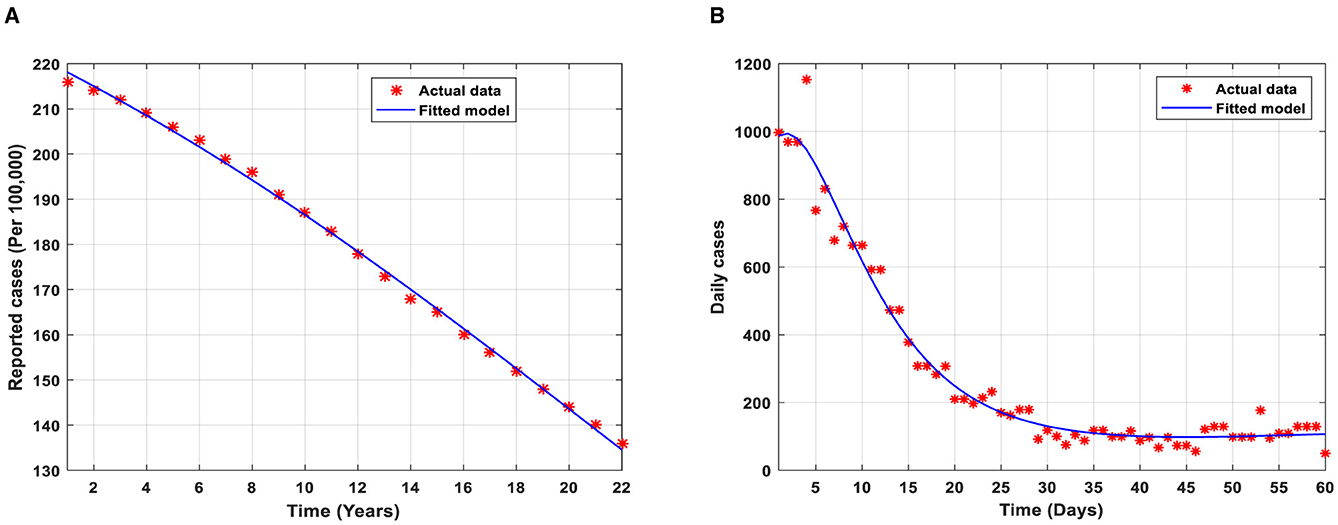
Figure 2. Plot of (A) TB stream (B) COVID-19 stream.

Table 1

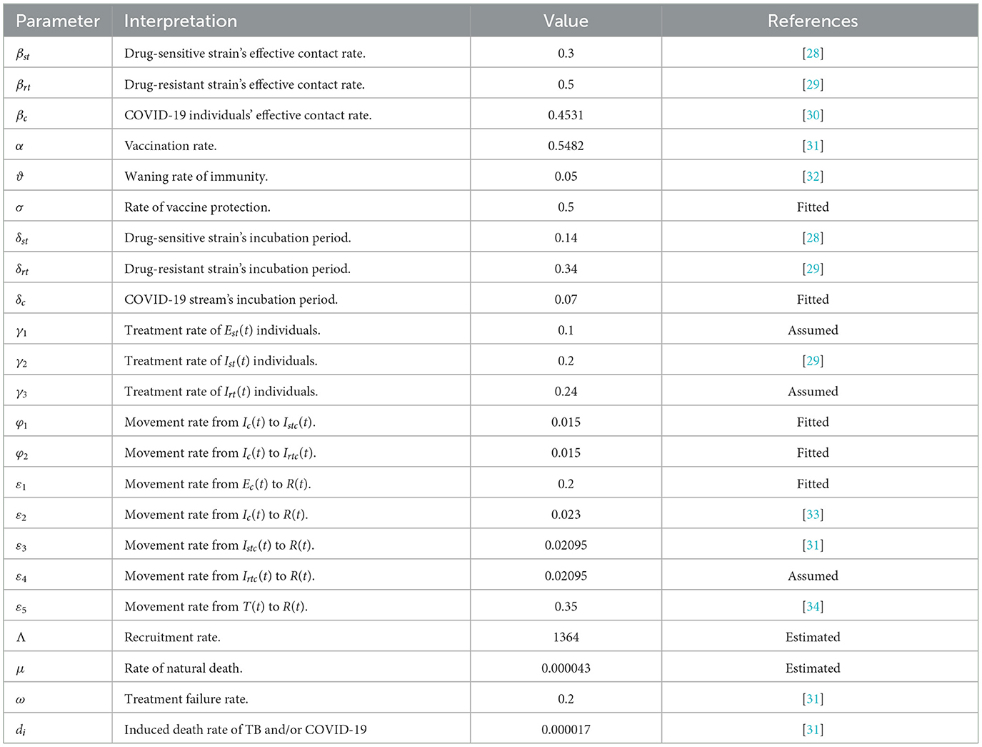
Table 1. Interpretation and values of model parameters.

Now, we investigate the relationship between the parameters and I_st, I_rt, and I_c by considering the behavioral patterns of the respective parameters associated with the drug-sensitive strain of TB, drug-resistant strain of TB, and COVID-19 stream on the reproduction numbers R_st, R_rt, and R_0c with the graphical representations illustrated below.

Figure 3A shows the partial rank correlation coefficients (PRCC) of the parameters associated with R_st which depicts the transmission dynamics of individuals who are infectious with drug-sensitive (DS) strains of TB only. It is observed that (β_st, δ_st) have a high positive effect on R_st. However, the vaccination protection rate σ is positive, this indicates that, the efficacy of the vaccine may be low. The parameters (α, γ₁, μ, ϑ) have a negative effect on R_st. Figure 3B shows the partial rank correlation coefficients (PRCCs) of the parameters associated with R_rt which depicts the transmission dynamics of the individuals infectious with drug-resistant (DR) strains of TB only. It is observed that (β_rt, δ_rt, ϑ) have a high positive impact on the reproduction number R_rt This indicates that majority of the individuals may be resistant to the drug. The parameters (α, γ₂, μ) have a negative impact on the reproduction number R_rt. Figure 3C shows the partial rank correlation coefficients (PRCCs) of the parameters associated with R_0C, which depicts the behavioral patterns of transmission of the individuals infectious with COVID-19 only. It is observed that (β_c, δ_c, ϑ) have a high positive effect on R_0C. Again, the vaccination protection rate σ is positive, this indicates that the efficacy of the vaccine may be low. This is determined by the associated sign; those with the positive sign indicate a perfect relationship and the negative sign indicates an imperfect relationship. If the value is high, then there exists a strong relationship, and the lower the value, the weaker the relation between the input and the output value. Once the vaccination protection rate σ increases, the reproduction numbers, and there should be measures to optimally control the transmission of TB and/or COVID-19.

Figure 3

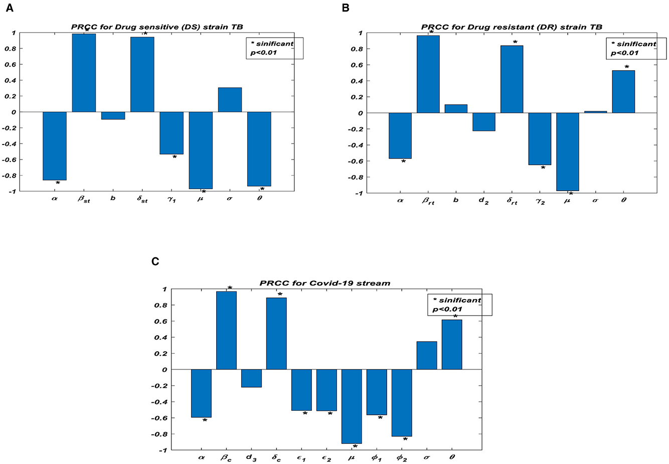
Figure 3. Partial rank correlation (PRCC) of the parameters in reproduction numbers. (A) PRCC for drug sensitive (DS) strain TB. (B) PRCC for drug resistant (DR) strain TB. (C) PRCC for COVID-19 stream.

To formulate control strategies to minimize the spread of TB and COVID-19, we demonstrate the transmission dynamics in different scenarios in the figures below based on the parameters that exhibit a strong relationship with the reproduction numbers, as demonstrated in Figure 4.

Figure 4

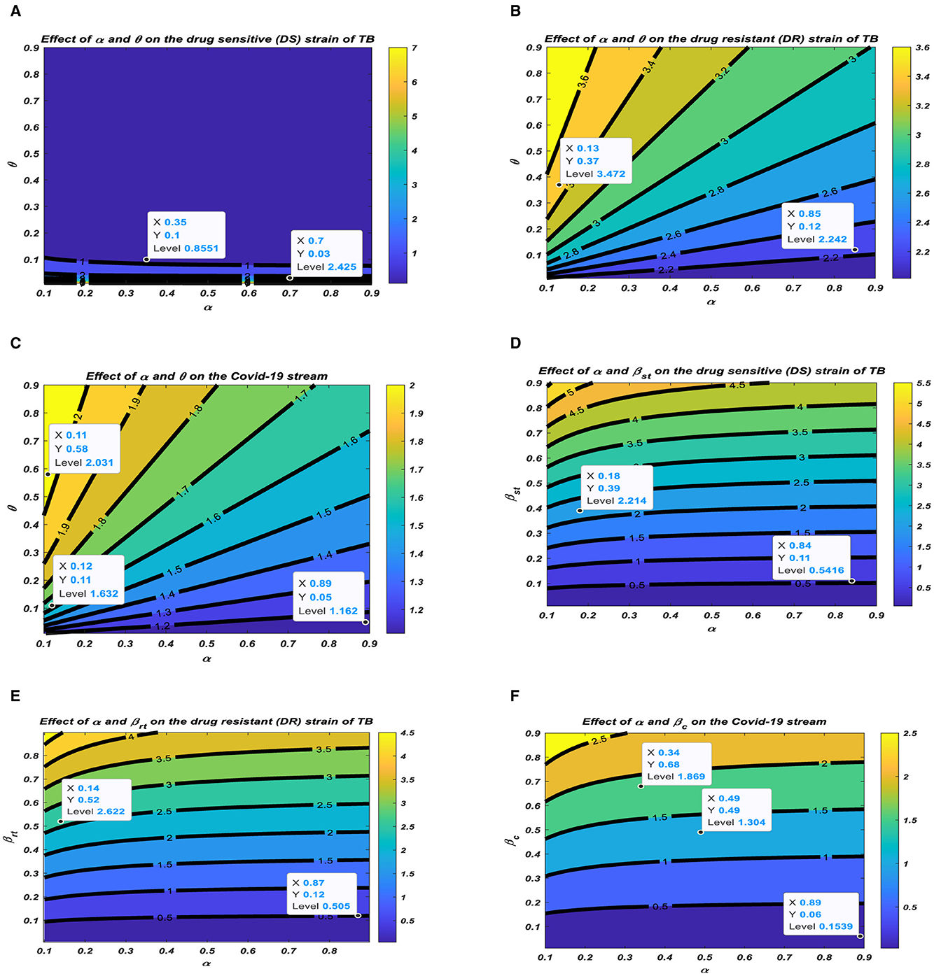
Figure 4. Relationship between the reproduction numbers and their corresponding parameters. (A) Effect of α and θ on the drug sensitive (DS) strain of TB. (B) Effect of α and θ on the drug resistant (DR) strain of TB. (C) Effect of α and θ on the COVID-19 stream. (D) Effect of α and β_st on the drug sensitive (DS) strain of TB. (E) Effect of α and β_rt on the drug resistant (DR) strain of TB. (F) Effect of α and β_c on the COVID-19 stream.

Figures 4A–C represent the respective contour plots of the reproduction numbers R_st, R_rt, and R_0C as a function of vaccination rate α and waning rate ϑ of vaccines. Figures 4D–F represent the respective contour plots of the reproduction numbers R_st, R_rt, and R_0C as a function of vaccination rate α and effective contact rates of TB and COVID-19. These figures suggest that to significantly minimizing the basic reproduction number to a minimum requires both pharmaceutical, such as vaccination, and non-pharmaceutical measures, such as mask usage and social distancing, to reduce the effective contact rate to prolong the period of acquiring the disease, which reduces the incubation rates.

All the above illustrations clearly show the pattern of the PRCC plots in Figure 3, and it is realized that all these parameters have either positive or negative effects on the transmission of TB and/or COVID-19. There should be effective interventions to reduce the rate of secondary infections; thus, R_st, R_rt, and R_0C of TB and COVID-19 co-infection.

Analysis of optimal control

We modify model (2) [see Equation (22)] with the following optimal control variable U₁(t), as public education on the prevention of TB and COVID-19, such as mask usage and social distancing, where U₁(t) ∈ [0, 1], which reduces the force of infection, λ₁, by 1 − U₁(t). U₂(t); control efforts to intensify vaccination of the population.U₃(t); control effort for case finding to enhance prophylaxis for the population by 1 + U₃(t). Hence, those identified as infectious will go through prophylaxis to minimize the infections that may occur. The control effort U₄(t) is control for case holding to control the failure of prophylaxis to minimize the reoccurrence of the disease by 1 − U₄(t). All these efforts denote the admissible control measures necessary to minimize the transmission of the diseases. The modified equation is given as

$\begin{array}{cc}\{\begin{array}{c}\frac{dS}{dt}=\Lambda +\vartheta V-\left[(1-U_1)({\rho }_1+{\rho }_2+{\rho }_3+{\rho }_4+{\rho }_5)+U_2\alpha +\mu \right]S,\\ \frac{dV}{dt}=U_2\alpha S-\left[(1-U_1)({\rho }_1+{\rho }_2+{\rho }_3+{\rho }_4+{\rho }_5)\sigma +\mu +\vartheta \right]V,\\ \frac{d{E}_{st}}{dt}=(1-U_1)(S+\sigma V){\rho }_1+{\rho }_2\omega T-(\mu +{\delta }_{st}+(1+U_3){\gamma }_1)E_{st},\\ \frac{d{I}_{st}}{dt}=(1-U_1)(S+\sigma V){\rho }_2+{\rho }_1\omega T+{\delta }_{st}{E}_{st}+\\ g{\epsilon }_3{I}_{stc}-(\mu +d_1+(1-U_4){\gamma }_2)I_{st},\\ \frac{d{E}_{rt}}{dt}=(1-U_1)(S+\sigma V){\rho }_3+\\ {\rho }_2\omega T-(\mu +{\delta }_{rt})E_{rt},\\ \frac{d{I}_{rt}}{dt}=(1-U_1)(S+\sigma V){\rho }_4+{\rho }_1\omega T+\\ {\delta }_{rt}{E}_{rt}+h{\epsilon }_3{I}_{rtc}-(\mu +d_2+(1-U_4){\gamma }_3)I_{rt},\\ \frac{d{E}_c}{dt}=(1-U_1)(S+\sigma V){\rho }_5-(\mu +{\delta }_c+(1+U_3){\epsilon }_1)E_c,\\ \frac{d{I}_c}{dt}={\delta }_c{E}_c-(\mu +d_3+{\phi }_1+{\phi }_2+{\epsilon }_2)I_c,\\ \frac{d{I}_{stc}}{dt}={\phi }_1{I}_c+(1-U_4)k{\gamma }_2{I}_{st}-(\mu +d_4+{\epsilon }_3)I_{stc},\\ \frac{d{I}_{rtc}}{dt}={\phi }_2{I}_c+(1-U_4)m{\gamma }_3{I}_{rt}-(\mu +d_5+{\epsilon }_4)I_{rtc},\\ \frac{dT}{dt}=(1+U_3){\gamma }_1{E}_{st}+(1-U_4)(1-k){\gamma }_2{I}_{st}+\\ (1-U_4)(1-m){\gamma }_3{I}_{rt}-(\mu +{\epsilon }_5+\omega {\lambda }_1)T,\\ \frac{dR}{dt}=(1+U_3){\epsilon }_1{E}_c+{\epsilon }_2{I}_c+(1-g)\\ {\epsilon }_3{I}_{stc}+(1-h){\epsilon }_4{I}_{rtc}+{\epsilon }_{5}T-\mu R.\end{array}& (22)\end{array}$

where ${\rho }_1=\frac{(1-b){\beta }_{st}{I}_{st}}{N},{\rho }_2=\frac{b{\beta }_{st}{I}_{st}}{N},{\rho }_3=\frac{(1-b){\beta }_{rt}{I}_{rt}}{N},{\rho }_4=\frac{b{\beta }_{rt}{I}_{rt}}{N}$, and ${\rho }_5=\frac{{\beta }_c{I}_c}{N}$ are derived from Section 2 with the initial conditions given in model (2).

Objective functional

We now formulate the optimal trajectories that show the effect of the control efforts U₁(t), U₂(t), U₃(t), U₄(t) subjected to Equation (22); the objective functional M is given as,

$\begin{array}{c}M\left(U_1,U_2,U_3,U_4\right)={\int }_0^{t_f}[m_1{E}_{st}+m_2{I}_{st}+\\ m_3{E}_{rt}+m_4{I}_{rt}+m_5{E}_c+m_6{I}_c+m_7{I}_{stc}+m_8{I}_{rtc}+\\ \frac{1}{2}{c}_1{U}_1^2\left(t\right)+\frac{1}{2}{c}_2{U}_2^2\left(t\right)+\\ \frac{1}{2}{c}_3{U}_3^2\left(t\right)+\frac{1}{2}{c}_4{U}_4^2\left(t\right)]dt.& (23)\end{array}$

We focus on minimizing the cost function (23), and the total cost of implementing the optimal control is given as

$\begin{array}{c}Q=\\ {\int }_0^{t_f}\left[\frac{1}{2}{c}_1{U}_1^2(t)+\frac{1}{2}{c}_1{U}_2^2(t)+\frac{1}{2}{c}_3{U}_3^2(t)+\frac{1}{2}{c}_4{U}_4^2(t)\right]dt.& (24)\end{array}$

The parameters c₁, c₂, c₃, and c₄ in Equation (24) are the balancing cost factors for U₁(t), U₂(t), U₃(t), U₄(t), respectively. All the control efforts U₁(t), U₂(t), U₃(t), U₄(t) are assumed to be bounded by Lebesgue measurable time-dependent functions on the interval [0, t_f], where t_f is the final time.

By Pontryagin's maximum principle, system (22) and the objective functional (23) are transformed into a state of point-wise Hamiltonian H. The following optimal solution is achieved.

$\begin{array}{c}H=m_1{E}_{st}+m_2{I}_{st}+m_3{E}_{rt}+m_4{I}_{rt}+m_5{E}_c+m_6{I}_c+m_7{I}_{stc}+\\ m_8{I}_{rtc}+\frac{1}{2}{c}_1{U}_1^2\left(t\right)+\frac{1}{2}{c}_2{U}_2^2\left(t\right)+\\ \frac{1}{2}{c}_3{U}_3^2\left(t\right)+\frac{1}{2}{c}_4{U}_4^2\left(t\right)+\\ {\lambda }_S(\Lambda +\vartheta V-[\left(1-U_1\right)({\rho }_1+{\rho }_2+{\rho }_3+{\rho }_4+{\rho }_5)+\\ U_2\alpha +\mu ]S)+{\lambda }_V(U_2\alpha S-[\left(1-U_1\right)\\ ({\rho }_1+{\rho }_2+{\rho }_3+{\rho }_4+{\rho }_5)\sigma +\\ \mu +\vartheta ]V)+{\lambda }_{E_{st}}(\left(1-U_1\right)\\ \left(S+\sigma V\right){\rho }_1+{\rho }_2\omega T-(\mu +{\delta }_{st}+\left(1+U_3\right){\gamma }_1)E_{st})+\\ {\lambda }_{I_{st}}(\left(1-U_1\right)\left(S+\sigma V\right){\rho }_2+{\rho }_1\omega T+\\ {\delta }_{st}{E}_{st}+g{\epsilon }_3{I}_{stc}-(\mu +d_1+(1-U_4){\gamma }_2)I_{st})+\\ {\lambda }_{E_{rt}}\left(\left(1-U_1\right)\left(S+\sigma V\right){\rho }_3+{\rho }_2\omega T-(\mu +{\delta }_{rt})E_{rt}\right)+\\ {\lambda }_{I_{rt}}(\left(1-U_1\right)\left(S+\sigma V\right){\rho }_4+{\rho }_1\omega T+{\delta }_{rt}{E}_{rt}+\\ h{\epsilon }_3{I}_{rtc}-(\mu +d_2+(1-U_4){\gamma }_3)I_{rt})+\\ {\lambda }_{E_c}\left(\left(1-U_1\right)\left(S+\sigma V\right){\rho }_5-(\mu +{\delta }_c+\left(1+U_3\right){\epsilon }_1)E_c\right)\\ +{\lambda }_{I_c}\left({\delta }_c{E}_c-(\mu +d_3+{\phi }_1+{\phi }_2+{\epsilon }_2)I_c\right)+\\ {\lambda }_{I_{stc}}\left({\phi }_1{I}_c+(1-U_4)k{\gamma }_2{I}_{st}-(\mu +d_4+{\epsilon }_3)I_{stc}\right)+\\ {\lambda }_{I_{rtc}}\left({\phi }_2{I}_c+(1-U_4)m{\gamma }_3{I}_{rt}-(\mu +d_5+{\epsilon }_4)I_{rtc}\right)+\\ {\lambda }_T(\left(1+U_3\right){\gamma }_1{E}_{st}+(1-U_4)\left(1-k\right){\gamma }_2{I}_{st}+\\ (1-U_4)\left(1-m\right){\gamma }_3{I}_{rt}-\left({\epsilon }_5+\omega {\lambda }_1\right)T)+\\ {\lambda }_R(\left(1+U_3\right){\epsilon }_1{E}_c+{\epsilon }_2{I}_c+\left(1-g\right){\epsilon }_3{I}_{stc}+\\ \left(1-h\right){\epsilon }_4{I}_{rtc}+{\epsilon }_{5}T-\mu R).& (25)\end{array}$

Where λ_S, λ_V, λ_Est, λ_Ist, λ_Ert, λ_Irt, λ_Ec, λ_Ic, λ_Istc, λ_Irtc, λ_T, λ_R in Equation (25) are the costate variables with respect to the state variables, S, V, E_st, I_st, E_rt, I_rt, E_c, I_c, I_stc, I_rtc, T, R.

Theorem 3: Given $U_1^{*}(t),U_2^{*}(t),U_3^{*}(t),U_4^{*}(t)$ as the optimal controls and the corresponding solutions $S^0,V^0,E_{st}^0,I_{st}^0,E_{rt}^0,I_{rt}^0,{E_c^0,I_c^0,I_{stc}^0,I_{rtc}^0,T}^0,R^0$ of system (22), which minimizes Q(U₁(t), U₂(t), U₃(t), U₄(t)), then there exist costate variables λ_S, λ_V, λ_Est, λ_Ist, λ_Ert, λ_Irt, λ_Ec, λ_Ic, λ_Istc, λ_Irtc, λ_T, λ_R that satisfy

$\begin{array}{cc}\frac{d{\lambda }_j}{dt}=-\frac{\partial H}{\partial j}.& (26)\end{array}$

With conditions λ_j(t_f) = 0, in (27) where j = S, V, E_st, I_st, E_rt, I_rt, E_c, I_c, I_stc, I_rtc, T, R, the optimality conditions that minimize the Hamiltonian, H, of (25) with respect to the controls are given as

$\begin{array}{cc}\{\begin{array}{c}{U}_1^{\ast }(t)=\\ \min \{U_{1}max,max\\ (0,\frac{(S^0+\sigma V^0)(({\lambda }_{E_{st}}-{\lambda }_S){\rho }_1+({\lambda }_{I_{st}}-{\lambda }_S){\rho }_2+({\lambda }_{E_{rt}}-{\lambda }_S){\rho }_3+({\lambda }_{I_{rt}}-{\lambda }_S){\rho }_4+({\lambda }_{E_c}-{\lambda }_S){\rho }_5)}{C_1})\},\\ U_2^{\ast }(t)=\min {\{U_{2}max,max(0,\frac{({\lambda }_S-{\lambda }_V)\alpha S^0}{C_2})\}}^{\prime }\\ U_3^{\ast }(t)=\min \{U_{3}max,max(0,\frac{({\lambda }_{E_{st}}-{\lambda }_T){\gamma }_1{E}_{st}^0-{\epsilon }_1{\lambda }_{E_c}{E}_c^0}{C_3})\},\\ U_4^{\ast }(t)=\min \{U_{4}max,max(0,\frac{({\lambda }_{I_{stc}}+{\lambda }_T-{\lambda }_{I_{st}}){\gamma }_2{I}_{st}^0+({\lambda }_{I_{rtc}}+{\lambda }_T-{\lambda }_{I_{rt}}){\gamma }_3{I}_{rt}^0}{C_4})\}.\end{array}& (27)\end{array}$

Proof: We take the partial derivative of Equation (25) with respect to the solutions of the system, optimal control, and final time conditions. The adjoint equation is demonstrated below in Equation (28).

$\begin{array}{cc}\{\begin{array}{c}\frac{d{\lambda }_S}{dS}=\left[1-U_1\right]\left[({\lambda }_{E_{st}}-{\lambda }_S){\rho }_1+({\lambda }_{I_{st}}-{\lambda }_S){\rho }_2+({\lambda }_{E_{rt}}-{\lambda }_S){\rho }_3+({\lambda }_{I_{rt}}-{\lambda }_S){\rho }_4+({\lambda }_{E_c}-{\lambda }_S){\rho }_5\right]+\\ ({\lambda }_V-{\lambda }_S)U_2\alpha +({\lambda }_S-{\lambda }_V)\vartheta V+\mu {\lambda }_S,\\ \frac{d{\lambda }_V}{dV}=\left[1-U_1\right]\left[({\lambda }_{E_{st}}-{\lambda }_V){\rho }_1+({\lambda }_{I_{st}}-{\lambda }_V){\rho }_2+({\lambda }_{E_{st}}-{\lambda }_T){\rho }_3+({\lambda }_{I_{rt}}-{\lambda }_V){\rho }_4+({\lambda }_{E_c}-{\lambda }_V){\rho }_5\right]\sigma +\\ ({\lambda }_V-{\lambda }_S)U_2\alpha S+({\lambda }_S-{\lambda }_V)\vartheta +\mu {\lambda }_V,\\ \frac{d{\lambda }_{E_{st}}}{d{E}_{st}}=-m_1+\left[1-U_1\right]\left[({\lambda }_{E_{st}}-{\lambda }_S)S+({\lambda }_{E_{st}}-{\lambda }_v)\sigma V\right]{\rho }_1+({\lambda }_{E_{st}}-{\lambda }_T){\rho }_2\omega T+({\lambda }_{I_{st}}-{\lambda }_{E_{st}}){\delta }_{st}+({\lambda }_T-{\lambda }_{E_{st}})\\ (1+U_3){\gamma }_1+\mu {\lambda }_{E_{st}},\\ \frac{d{\lambda }_{I_{st}}}{d{I}_{st}}=-m_2+\left[1-U_1\right]\left[({\lambda }_{I_{st}}-{\lambda }_S)S+({\lambda }_{I_{st}}-{\lambda }_v)\sigma V\right]{\rho }_2+({\lambda }_{I_{st}}-{\lambda }_T){\rho }_1\omega T+({\lambda }_{I_{st}}-{\lambda }_{E_{st}}){\delta }_{st}{E}_{st}+\\ ({\lambda }_T-{\lambda }_{I_{st}})(1-U_4)(1-k){\gamma }_2+({\lambda }_{I_{st}}-{\lambda }_{I_{stc}})g{\epsilon }_3{I}_{stc}+({\lambda }_{I_{stc}}-{\lambda }_{I_{st}})(1-U_4)k{\gamma }_2+(\mu +d_1){\lambda }_{I_{st}},\\ \frac{d{\lambda }_{E_{rt}}}{d{E}_{rt}}=-m_3+\left[1-U_1\right]\left[({\lambda }_{E_{rt}}-{\lambda }_S)S+({\lambda }_{E_{rt}}-{\lambda }_v)\sigma V\right]{\rho }_3+({\lambda }_{E_{rt}}-{\lambda }_T){\rho }_4\omega T+({\lambda }_{I_{rt}}-{\lambda }_{E_{rt}}){\delta }_{rt}+\mu {\lambda }_{E_{rt}},\\ \frac{d{\lambda }_{I_{rt}}}{d{I}_{rt}}=-m_4+\left[1-U_1\right]\left[({\lambda }_{I_{rt}}-{\lambda }_S)S+({\lambda }_{I_{rt}}-{\lambda }_v)\sigma V\right]{\rho }_4+({\lambda }_{I_{rt}}-{\lambda }_T){\rho }_3\omega T+({\lambda }_{I_{rt}}-{\lambda }_{I_{rtc}})h{\epsilon }_4{I}_{rtc}+\\ ({\lambda }_{I_{rtc}}-{\lambda }_{I_{rt}})(1-U_4)(1-m){\gamma }_3+({\lambda }_T-{\lambda }_{I_{rt}})(1-U_4)(1-m){\gamma }_3+(\mu +d_2){\lambda }_{I_{rt}},\\ \frac{d{\lambda }_{E_c}}{d{E}_c}=-m_5+\left[1-U_1\right]\left[({\lambda }_{E_c}-{\lambda }_S)S+({\lambda }_{E_c}-{\lambda }_v)\sigma V\right]{\rho }_5+({\lambda }_{I_c}-{\lambda }_{E_c}){\delta }_c+({\lambda }_R-{\lambda }_{E_c})(1+U_3){\epsilon }_1+\mu {\lambda }_{E_c},\\ \frac{d{\lambda }_{I_c}}{d{I}_c}=-m_6+({\lambda }_{I_c}-{\lambda }_{E_c}){\delta }_c{E}_c+({\lambda }_{I_{stc}}-{\lambda }_{I_c}){\phi }_1+({\lambda }_{I_{rtc}}-{\lambda }_{I_c}){\phi }_2+({\lambda }_R-{\lambda }_{I_c}){\epsilon }_2+(\mu +d_3){\lambda }_{I_c},\\ \frac{d{\lambda }_{I_{stc}}}{d{I}_{stc}}=-m_7+({\lambda }_{I_{stc}}-{\lambda }_{I_c}){\phi }_1{I}_c+({\lambda }_{I_{stc}}-{\lambda }_{I_{st}})(1-U_4)k{\gamma }_2{I}_{st}+({\lambda }_{I_{st}}-{\lambda }_{I_{stc}})g{\epsilon }_3+({\lambda }_R-{\lambda }_{I_{stc}})(1-g){\epsilon }_3+(\mu +d_4){\lambda }_{I_{stc}},\\ \frac{d{\lambda }_{I_{rtc}}}{d{I}_{rtc}}=-m_8+({\lambda }_{I_{rtc}}-{\lambda }_{I_c}){\phi }_2{I}_c+({\lambda }_{I_{rtc}}-{\lambda }_{I_{rt}})h{\epsilon }_4{I}_{rt}+({\lambda }_{I_{rt}}-{\lambda }_{I_{rtc}})(1-U_4)m{\gamma }_3+({\lambda }_R-{\lambda }_{I_{rtc}})(1-h){\epsilon }_4+(\mu +d_5){\lambda }_{I_{rtc}},\\ \frac{d{\lambda }_T}{dT}=({\lambda }_T-{\lambda }_{E_{st}})(1+U_3){\gamma }_1{E}_{st}+({\lambda }_T-{\lambda }_{I_{st}})(1-U_4)(1-k){\gamma }_2{I}_{st}+({\lambda }_T-{\lambda }_{I_{rt}})(1-U_4)(1-m){\gamma }_3{I}_{rt}+({\lambda }_{E_{st}}-{\lambda }_T){\rho }_2\omega \\ ({\lambda }_{I_{st}}-{\lambda }_T){\rho }_1\omega +({\lambda }_{E_{rt}}-{\lambda }_T){\rho }_4\omega +({\lambda }_{I_{rt}}-{\lambda }_T){\rho }_3\omega +({\lambda }_R-{\lambda }_T){\epsilon }_5+\mu {\lambda }_T,\\ \frac{d{\lambda }_R}{dR}=({\lambda }_R-{\lambda }_{E_c})(1+U_3){\epsilon }_1{E}_c+({\lambda }_R-{\lambda }_{I_c}){\epsilon }_2{I}_c+({\lambda }_R-{\lambda }_{I_{stc}})(1-g){\epsilon }_3{I}_{stc}+({\lambda }_R-{\lambda }_{I_{rtc}})(1-h){\epsilon }_4{I}_{rtc}+({\lambda }_R-{\lambda }_T){\epsilon }_{5}T+\mu {\lambda }_R.\end{array}& (28)\end{array}$

The control set Equation (29) below illustrates the costate system with the optimal conditions.

$\begin{array}{cc}\{\begin{array}{c}\frac{\partial H}{\partial U_1}=C_1{U}_1+\left(S^0+\sigma V^0\right)\\ (\left({\lambda }_S-{\lambda }_{E_{st}}\right){\rho }_1+\left({\lambda }_S-{\lambda }_{I_{st}}\right){\rho }_2+\\ \left({\lambda }_S-{\lambda }_{E_{rt}}\right){\rho }_3+\left({\lambda }_S-{\lambda }_{I_{rt}}\right){\rho }_4+\left({\lambda }_S-{\lambda }_{E_c}\right){\rho }_5),\\ \frac{\partial H}{\partial U_2}=C_2{U}_2+\left({\lambda }_V-{\lambda }_S\right)\alpha S^0,\\ \frac{\partial H}{\partial U_3}=C_3{U}_3+\left({\lambda }_T-{\lambda }_{E_{st}}\right){\gamma }_1{E}_{st}^0+{\epsilon }_1{E}_c^0{\lambda }_{E_c},\\ \frac{\partial H}{\partial U_4}=C_4{U}_4+\left({\lambda }_{I_{st}}-{\lambda }_T-{\lambda }_{I_{stc}}\right){\gamma }_2{I}_{st}^0+\left({\lambda }_{I_{rt}}-{\lambda }_T-{\lambda }_{I_{rtc}}\right){\gamma }_3{I}_{rt}^0.\end{array}& (29)\end{array}$

We solve for $U_1(t),U_2(t),U_3(t),and{U}_4(t)as{U}_1^{*}(t),$ $U_2^{*}(t),U_3^{*}(t),$ and $U_4^{*}(t)$ of Equation (25), and the results are given in Equation (30):

$\begin{array}{cc}\{\begin{array}{c}{U}_1^{*}(t)=\\ \frac{(S^0+\sigma V^0)(({\lambda }_{E_{st}}-{\lambda }_S){\rho }_1+({\lambda }_{I_{st}}-{\lambda }_S){\rho }_2+({\lambda }_{E_{rt}}-{\lambda }_S){\rho }_3+({\lambda }_{I_{rt}}-{\lambda }_S){\rho }_4+({\lambda }_{E_c}-{\lambda }_S){\rho }_5)}{C_1},\\ U_2^{*}(t)={\frac{({\lambda }_S-{\lambda }_V)\alpha S^0}{C_2}}^{\prime }\\ U_3^{*}(t)=\frac{({\lambda }_{E_{st}}-{\lambda }_T){\gamma }_1{E}_{st}^0-{\epsilon }_1{\lambda }_{E_c}{E}_c^0}{C_3},\\ U_4^{*}(t)=\frac{({\lambda }_{I_{stc}}+{\lambda }_T-{\lambda }_{I_{st}}){\gamma }_2{I}_{st}^0+({\lambda }_{I_{rtc}}+{\lambda }_T-{\lambda }_{I_{rt}}){\gamma }_3{I}_{rt}^0}{C_4}.\end{array}& (30)\end{array}$

Therefore, using the bounds of the controls $U_1^{*}(t),U_2^{*}(t),U_3^{*}(t),$ and $U_4^{*}(t),$ the control efforts are in the compact form given by the optimal condition of the system in (27); hence, the proof is complete.

Optimal control results

The goal of this subsection is to study the two strains of TB; thus, drug-sensitive (DS) and drug-resistant (DR) strains of TB influence COVID-19 using the control efforts. We explore the effects of implementing the control efforts; therefore, the optimality system (21) is solved forward in time and the adjoint system backward in time with the corresponding lower and upper bounds of the controls. We use the population of Ghana to study the behavioral pattern of the co-infection of TB and COVID-19. The estimated total population of Ghana is 31732129 [35]; hence, N(0) = 31732129, and the assumed initial values are as follows: S(0) = 20000000, V(0) = 100000, E_st(0) = 20000, I_st(0) = 10000, E_rt(0) = 20000, I_rt(0) = 10000, E_c(0) = 15000, I_c(0) = 10000, I_stc(0) = 20000, I_rtc(0) = 20000, T = (0)100000, R(0) = 5000, together with parameter values illustrated in Table 1. The balance costs associated with the objective functional are assumed as C₁ = 200, C₂ = 100, C₃ = 500, C₄ = 1000 and weights m_i = 100, where i = 1, 2, 3, 4, 5, 6, 7, 8. The lower bound (LB) and upper bound (UB) are assumed as LB₁ = 0, UB₁ = 1, LB₂ = 0, UB₂ = 1, LB₃ = 0, UB₃ = 1. The results are illustrated according to the strategies to implement the control efforts.

Strategy 1: implementation of public education (U₁)

This intervention is most favorable for both streams of diseases, thus halting the transmission of TB and COVID-19. The optimal solutions illustrated in Figure 5 account for the observations when the control effort U₁ is applied accordingly.

Figure 5

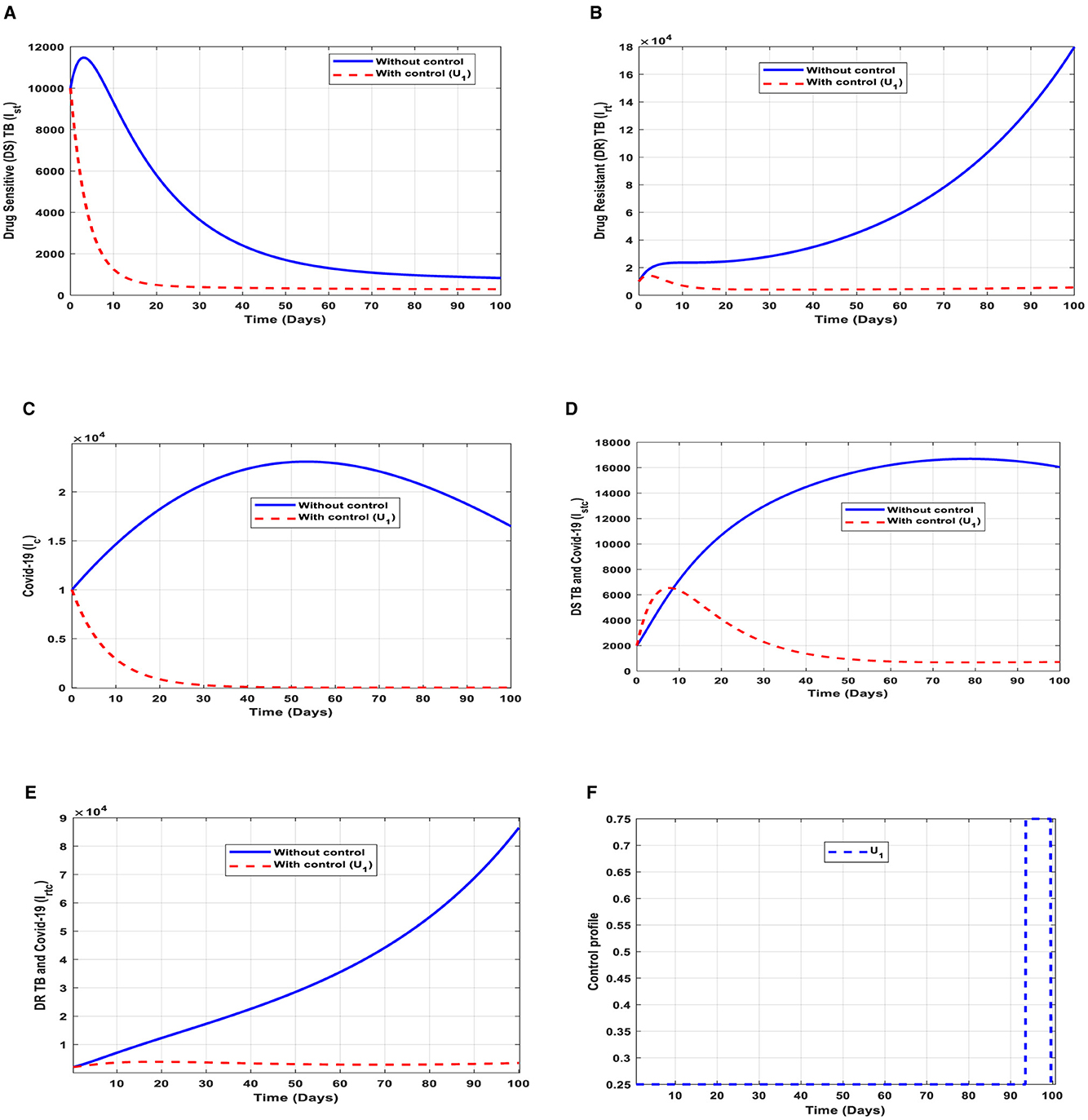
Figure 5. (A–E) Red dotted line is the optimal solution for implementing strategy 1. (F) Optimal control profile for strategy 1.

The optimal solutions illustrated above depict the following observations when public education is only applied.

(a) Figure 5A represents the effect of the control effort U₁ on the individuals infectious with drug-sensitive (DS) strain of TB only. This implies that the number of individuals will decrease to the minimum within 20 days if the control intervention is optimally implemented to halt the disease's transmission. Conversely, it will decrease but not significantly.

(b) Figure 5B represents the effect of the control effort U₁ on the individuals infectious with drug-resistant (DR) strain of TB only. This implies that the number of individuals will decrease to the minimum within 90 days if the control effort is optimally implemented to halt the disease's transmission. Conversely, if the control intervention is ignored, the number of infected individuals will increase significantly by>15, 000 per 100,000 people before the 90th day, which will result in the higher transmission of the drug-resistant (DR) strain of TB only in the individuals.

(c) Figure 5C represents the effect of the control effort U₁ on the individuals infectious with COVID-19 only. This implies that the number of individuals will decrease to the minimum within 30 days if the control effort is optimally implemented to halt the disease's transmission. Conversely, it will increase significantly.

(d) Figure 5D represents the effect of the control effort U₁ on the individuals infectious with drug-sensitive (DS) strain of TB and COVID-19 at the same time. This implies that the number of individuals will decrease to the minimum within extra days if the control effort is optimally implemented to halt the disease's transmission. Conversely, it will decrease but not significantly.

(e) Figure 5E represents the effect of the control effort U₁ on the individuals infectious with drug-resistant (DR) strain of TB and COVID-19 at the same time. This implies that the number of individuals will decrease to the minimum within 90 days if the control effort is optimally implemented to halt the transmission of the disease. Conversely, if the control intervention is ignored, the number of infected individuals will increase significantly by>90000 per 100000 people before the 90th day, which will result in higher transmission of the drug-resistant (DR) strain of TB and COVID-19 in the individuals.

(f) Figure 5F represents the profile of control efforts for public education on the prevention of TB and COVID-19, such as mask usage and social distancing. This implies that education should reach more than 25% of the population from the start of implementation and must be intensified and fully optimized to 100% after 85 subsequent days to minimize the transmission of TB and COVID-19.

Strategy 2: implementation of vaccination (U₂)

This intervention is also favorable for both streams of diseases, thus halting the spread of TB and COVID-19; however, it should be implemented with care because the proportion of the individuals may develop the drug-resistant (DR) strain of TB if treatment failure occurs, and the waning rate of the vaccine. The optimal solutions illustrated in Figure 6 account for the observations when the control effort U₂ is applied accordingly.

Figure 6

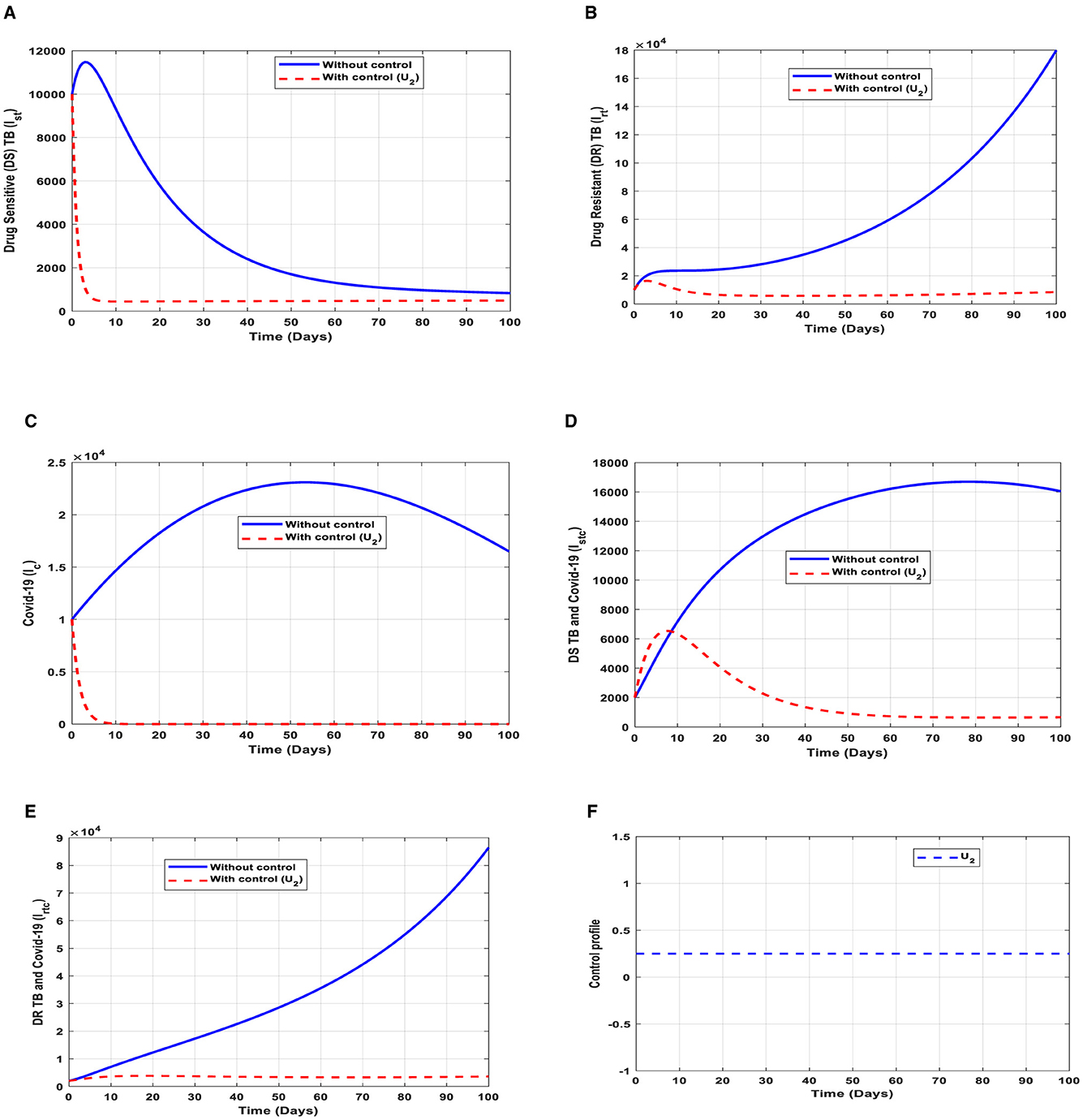
Figure 6. (A–E) Red dotted line is the optimal solution for implementing strategy 2. (F) Optimal control profile for strategy 2.

The optimal solutions illustrated above depict the following observations when vaccination is only applied.

(a) Figure 6A represents the effect of the control effort U₂ on the individuals infectious with drug-sensitive (DS) strain of TB only. This implies that the number of individuals will decrease to the minimum within 10 days if the control intervention is optimally implemented to halt the disease's transmission. Conversely, it will increase significantly.

(b) Figure 6B represents the effect of the control effort U₂ on the individuals infectious with drug-resistant (DR) strain of TB only. This implies that the number of individuals will decrease to the minimum within 90 days if the control intervention is optimally implemented to halt the disease's transmission. Conversely, if the control effort is ignored, the number of infected individuals will increase significantly by>15, 000 per 100,000 people before the 65th day, which will result in the higher transmission of the drug-resistant (DR) strain of TB only in the individuals. This is a result of drug resistance, which leads to treatment failure.

(c) Figure 6C represents the effect of the control effort U₂ on the individuals infectious with COVID-19 only. This implies that the number of individuals will decrease to the minimum within 10 days if the control effort is optimally implemented to halt the disease's transmission. Conversely, it will increase significantly.

(d) Figure 6D represents the effect of the control effort U₂ on the individuals infectious with drug-sensitive (DS) strain of TB and COVID-19 at the same time. This implies that the number of individuals will decrease to the minimum within extra days if the control effort is optimally implemented to halt the disease's transmission. Conversely, it will increase significantly.

(e) Figure 6E represents the effect of the control effort U₁ on the individuals infectious with drug-resistant (DR) strain of TB and COVID-19 at the same time. This implies that the number of individuals will decrease to the minimum within 60 days if the control intervention is optimally implemented to halt the disease's transmission. Conversely, if the control intervention is ignored, the number of infected individuals will increase significantly by>80, 000 per 100,000 people before the 90th day, which will result in higher transmission of the drug-resistant (DR) strain of TB and COVID-19 in the individuals. This is a result of drug resistance and vaccine inefficacy, which leads to treatment failure and/or reinfection.

(f) Figure 6F represents the profile of control efforts for vaccination to prevent TB and COVID-19. This implies that the vaccination needs to be intensified by more than 25% and reach the population from the start of implementation and must be intensified fully and optimized to 100% after some days throughout the subsequent days to halt both TB and COVID-19 transmission.

Strategy 3: implementation of case finding (U₃)

This intervention is also favorable for both streams of diseases, thus halting the spread of TB and COVID-19. The optimal solutions, illustrated in Figure 7, account for the observations when the control effort U₃ is applied accordingly.

Figure 7

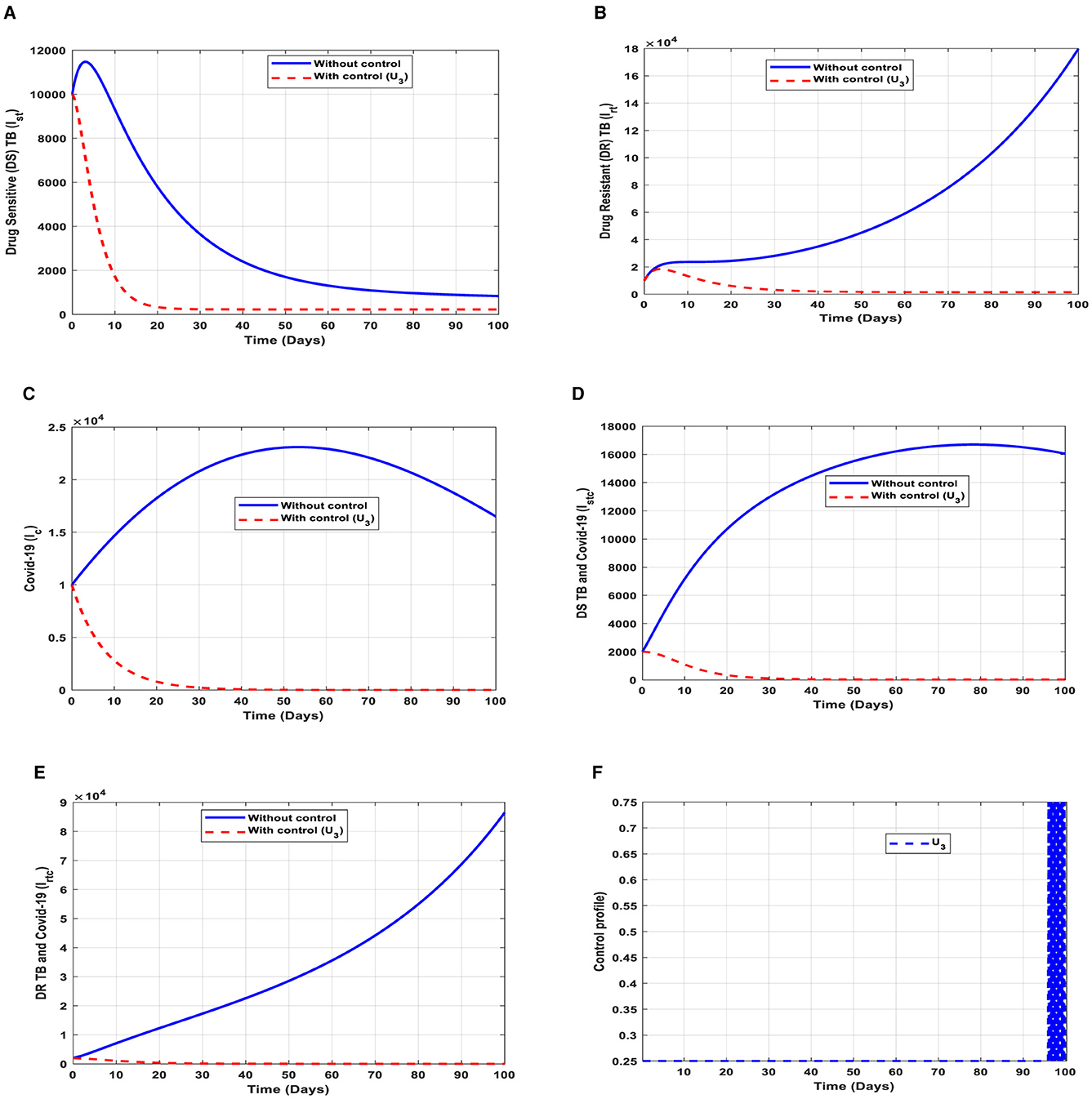
Figure 7. (A–E) Red dotted line is the optimal solution for implementing strategy 3. (F) Optimal control profile for strategy 3.

The optimal solutions illustrated above depict the following observations when case finding is only applied. This is mostly used to detect TB infection.

(a) Figure 7A represents the effect of the control effort U₃ on the individuals infectious with drug-sensitive (DS) strain of TB only. This implies that the number of individuals will decrease to the minimum within 20 days if the control intervention is optimally implemented to halt the disease's transmission. Conversely, it will increase significantly.

(b) Figure 7B represents the effect of the control effort U₃ on the individuals infectious with drug-resistant (DR) strain of TB only. This implies that the number of individuals will decrease to the minimum within 30 days if the control effort is optimally implemented to halt the transmission of the disease. Conversely, if the control intervention is ignored, the number of infected individuals will increase significantly by>150, 000 per 100,000 people before the 90th day, which will result in higher transmission of the drug-resistant (DR) strain of TB only in the individuals.

(c) Figure 7C represents the effect of the control effort U₃ on the individuals infectious with COVID-19 only. This implies that the number of individuals will decrease to the minimum within 30 days if the control effort is optimally implemented to halt the disease's transmission. Conversely, it will increase significantly.

(d) Figure 7D represents the effect of the control effort U₃ on the individuals infectious with drug-sensitive (DS) strain of TB and COVID-19 at the same time. This implies that the number of individuals will decrease to the minimum within 30 days if the control effort is optimally implemented to halt the disease's transmission. Conversely, it will increase significantly.

(e) Figure 7E represents the effect of the control effort U₃ on the individuals infectious with drug-resistant (DR) strain of TB and COVID-19 at the same time. This implies that the number of individuals will decrease to the minimum within 90 days if the control effort is optimally implemented to halt the disease's transmission. Conversely, if the control intervention is ignored, the number of infected individuals will increase significantly by>180, 000 per 100,000 people before the 90th day, which will result in higher transmission of the drug-resistant (DR) strain of TB and COVID-19 in the individuals.

(f) Figure 7F represents the profile of the control effort for finding cases of TB and COVID-19. This implies that ~25% of the cases should be identified for immediate treatment within 85 days of implementation and must be intensified to ~75% in the subsequent days to halt both TB and COVID-19 transmission. However, the latter days of implementation vary between 25% and 75% based on the outcome of this intervention.

Strategy 4: implementation of case holding (U₄)

This intervention is also favorable for both streams of diseases, thus halting the transmission of TB and COVID-19. The optimal solutions, illustrated in Figure 8, account for the observations when the control effort U₄ is applied accordingly.

Figure 8

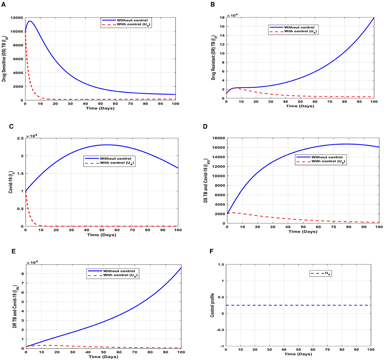
Figure 8. (A–E) Red dotted line is the optimal solution for implementing strategy 4. (F) Optimal control profile for strategy 4.

The optimal solutions illustrated above depict the following observations when case holding is only applied. This is also mostly used to handle TB infections.

(a) Figure 8A represents the effect of the control effort U₄ on the individuals infectious with drug-sensitive (DS) strain of TB only. This implies that the number of individuals will decrease to the minimum within 20 days if the control effort is optimally implemented to halt the disease's transmission. Conversely, it will increase significantly.

(b) Figure 8B represents the effect of the control effort U₄ on the individuals infectious with drug-resistant (DR) strain of TB only. This implies that the number of individuals will decrease to the minimum within 80 days if the control intervention is optimally implemented to halt the disease's transmission. Conversely, if the control effort is ignored, the number of infected individuals will increase significantly by>10, 000 per 100,000 people before the 90th day, which will result in higher transmission of the drug-resistant (DR) strain of TB only in the individuals.

(c) Figure 8C represents the effect of the control effort U₄ on the individuals infectious with COVID-19 only. This implies that the number of individuals will decrease to the minimum within 10 days if the control intervention is optimally implemented to halt the disease's transmission. Conversely, it will increase significantly.

(d) Figure 8D represents the effect of the control effort U₄ on the individuals infectious with drug-sensitive (DS) strain of TB and COVID-19 at the same time. This implies that the number of individuals will decrease to the minimum within 80 days if the control intervention is optimal to halt the disease's transmission. Conversely, it will increase significantly.

(e) Figure 8E represents the effect of the control effort U₄ on the individuals infectious with drug-resistant (DR) strain of TB and COVID-19 at the same time. This implies that the number of individuals will decrease to the minimum within 90 days if the control intervention is optimally implemented to halt the disease's transmission. Conversely, if the control effort is ignored, the number of infected individuals will increase significantly by>50, 000 per 100,000 people before the 90th day, which will result in higher transmission of the drug-resistant (DR) strain of TB and COVID-19 in the individuals. This intervention is normally used to handle individuals infectious with (DR) strain of TB because it is very difficult to treat them. Therefore, one could realize a decrease in the number of infections.

(f) Figure 8F represents the profile of control effort for case holding for TB and COVID-19. It implies that more than 25% of the cases should be handled properly among the population from the start of implementation and must be intensified fully and optimized to 100% after some days throughout the subsequent days to halt both TB and COVID-19 transmission.

Strategy 5: implementation of all controls (U₁, U₂, U₃, U₄)

These interventions are also favorable for both streams of diseases, thus halting the transmission of TB and COVID-19. The optimal solutions, illustrated in Figure 9, account for the observations when all the control efforts are applied accordingly.

Figure 9

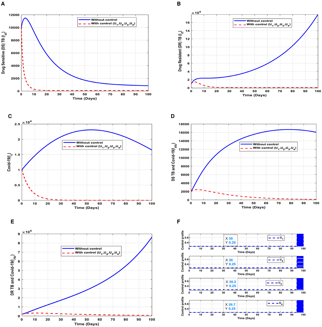
Figure 9. (A–E) Red dotted line is the optimal solution for implementing strategy 5. (F) Optimal control profile for strategy 5.

The optimal solutions illustrated above depict the following observations when all the control efforts are applied.

(a) Figure 9A represents the effect of all the control efforts U₁, U₂, U₃, U₄ on the individuals infectious with drug-sensitive (DS) strain of TB only. This implies that the number of individuals will decrease to the minimum within 20 days if the control interventions are optimally implemented to halt the disease's transmission. Conversely, it will increase significantly.

(b) Figure 9B represents the effect of all the control efforts U₁, U₂, U₃, U₄ on the individuals infectious with drug-resistant (DR) strain of TB only. This implies that the number of individuals will decrease to the minimum within 30 days if the control interventions are optimally implemented to halt the disease's transmission. Conversely, if the control effort is ignored, the number of infected individuals will increase significantly by>14000 people before the 50th day.

(c) Figure 9C represents the effect of all the control efforts U₁, U₂, U₃, U₄ on the individuals infectious with COVID-19 only. This implies that the number of individuals will decrease to the minimum within 30 days if the control effort is optimally implemented to halt the disease's transmission. Conversely, it will increase significantly.

(d) Figure 9D represents the effect of all the control efforts U₁, U₂, U₃, U₄ on the individuals infectious with drug-sensitive (DS) strain of TB and COVID-19 at the same time. This implies that the number of individuals will decrease to the minimum within 80 days if the control effort is optimally implemented to halt the disease's transmission. Conversely, it will increase significantly.

(e) Figure 9E represents the effect of all the control efforts U₁, U₂, U₃, U₄ on the individuals infectious with drug-resistant (DR) strain of TB and COVID-19 at the same time. This implies that the number of individuals will decrease to the minimum within 80 days if the control effort is optimally implemented to halt the disease's transmission. Conversely, if the control interventions are ignored, the number of infected individuals will increase significantly by>70000 per 100000 people before the 80th day, which will result in higher transmission of the drug-resistant (DR) strain of TB and COVID-19 in the individuals.

(f) Figure 9F represents the profile of control efforts for public education, vaccination, case finding, and case holding of TB and COVID-19. This implies that all the controls should be implemented at the same rate. Thus, ~25% of the population should be educated, vaccinated, cases should be identified for immediate treatment and hold the cases within 95 days of implementation, and should be intensified to ~70% in the subsequent days to halt both TB and COVID-19 transmission. However, the latter days of implementation vary between 25% and 70% based on the outcome of these interventions.

Strategy 6: implementation of public education and vaccination (U₁, U₂)

This intervention is also favorable for both streams of diseases, thus halting the transmission of TB and COVID-19. The optimal solutions, illustrated in Figure 10, account for the observations when the control efforts U₁, U₂ are applied accordingly.

Figure 10

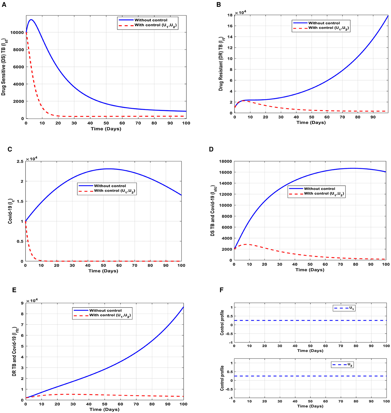
Figure 10. (A–E) Red dotted line is the optimal solution for implementing strategy 6. (F) Optimal control profile for strategy 6.

The optimal solutions illustrated above depict the following observations when all the control efforts are applied. These interventions are normally applied to COVID-19 infection only.

(a) Figure 10A represents the effect of the control efforts U₁, U₂ on the individuals infectious with drug-sensitive (DS) strain of TB only. This implies that the number of individuals will decrease but not to the minimum within 30 days if the control interventions are optimally implemented to halt the disease's transmission. On the other hand, it will increase significantly.

(b) Figure 10B represents the effect of the control efforts U₁, U₂ on the individuals infectious with drug-resistant (DR) strain of TB only. This implies that the number of individuals will decrease to the minimum within 90 days if the control efforts are optimally implemented to halt the transmission of the disease. Conversely, if the control interventions are ignored, the number of infected individuals will increase significantly by>140, 000 people before the 90th day but in decreasing order of drug-resistant (DR) strain of TB-only transmission in the individuals. This is a result of the probability of the individual developing resistance to the drug.

(c) Figure 10C represents the effect of the control efforts U₁, U₂ on the individuals infectious with COVID-19 only. This implies that the number of individuals will decrease to the minimum within 10 days if the control interventions are optimally implemented to halt the disease's transmission. Conversely, it will increase significantly. These strategies are ideal for COVID-19 infection only,

(d) Figure 10D represents the effect of the control efforts U₁, U₂ on the individuals infectious with drug-sensitive (DS) strain of TB and COVID-19 at the same time. This implies that the number of individuals will decrease to the minimum within extra days and may worsen the situation if the control efforts are optimally implemented. This is a result of not identifying infectious individuals, vaccine inefficacy, and drug resistance.

(e) Figure 10E represents the effect of the control efforts U₁, U₂, U₃, U₄ on the individuals infectious with drug-resistant (DR) strain of TB and COVID-19 at the same time. This implies that the number of individuals will decrease to the minimum within 90 days if the control interventions are optimally implemented to halt the transmission of the disease. Conversely, if the control interventions are ignored, the number of infected individuals will increase significantly by>70, 000 per 100,000 people before the 80th day, which will result in higher transmission of the drug-resistant (DR) strain of TB and COVID-19 in the individuals.

(f) Figure 10F represents the profile of control effort for public education and vaccination for TB and COVID-19. This implies that all the interventions U₁, U₂ should be more than 25% intensified in the population from the start of implementation and must be intensified fully and optimized to 100% after some days throughout the subsequent days; however, U₂ should be 25% throughout the implementation in halting both TB and COVID-19 transmission.

Strategy 7: implementation of case finding and case holding (U₃, U₄)

This intervention is also favorable for both streams of diseases, thus halting the spread of TB and COVID-19. The optimal solutions, illustrated in Figure 11, account for the observations when the control efforts U₃, U₄ are applied accordingly.

Figure 11

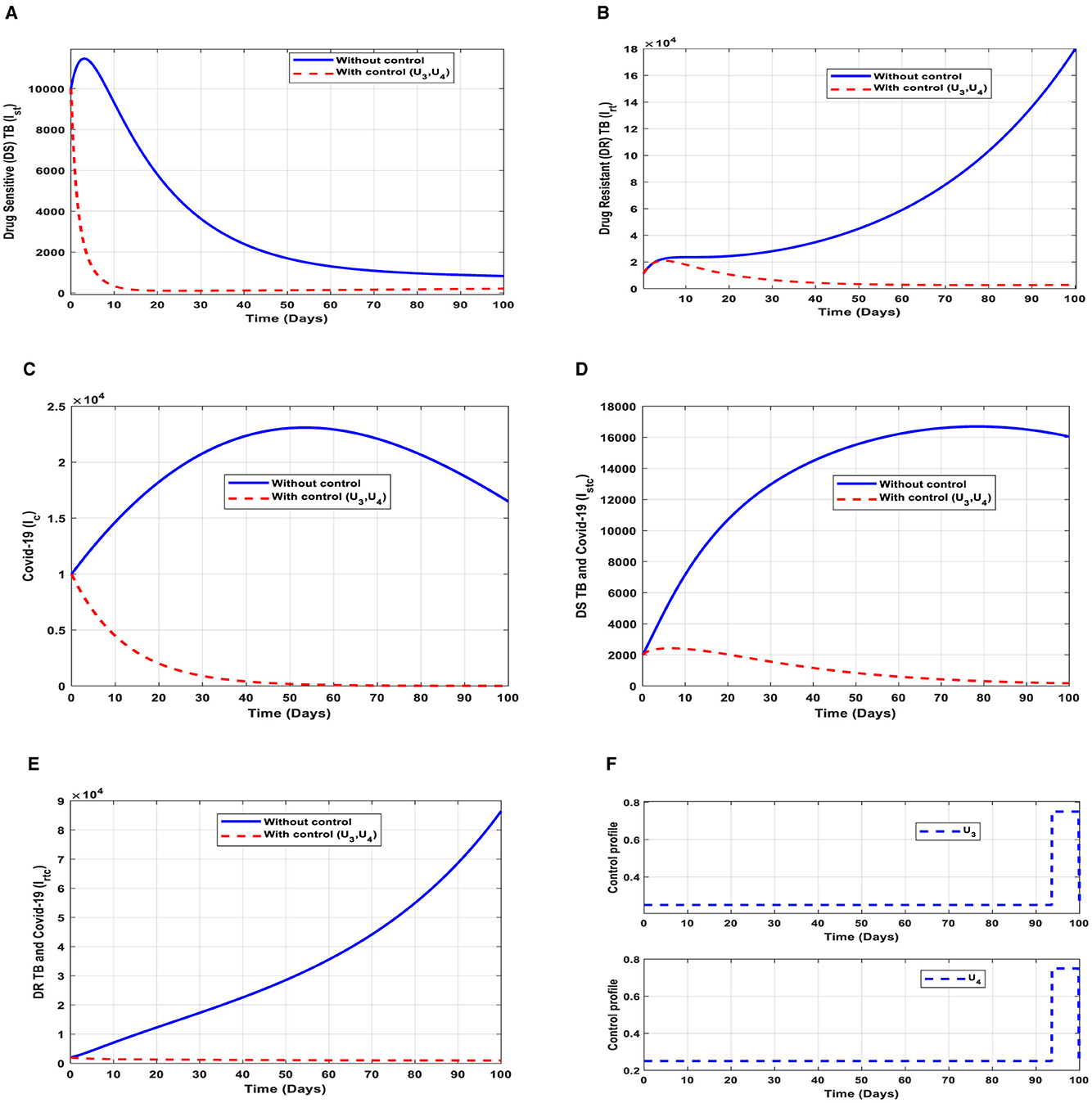
Figure 11. (A–E) Red dotted line is the optimal solution for implementing strategy 7. (F) Optimal control profile for strategy 7.

The optimal solutions illustrated above depict the following observations when public education is only applied. These interventions are normally applied to TB infection only.

(a) Figure 11A represents the effect of the control efforts U₃, U₄ on the individuals infectious with drug-sensitive (DS) strain of TB only. This implies that the number of individuals will decrease to the minimum within 20 days if the control interventions are optimally implemented to halt the disease's transmission. Conversely, it will increase. This is a result of identifying and holding the cases as early as possible to prevent further transmission.

(b) Figure 11B represents the effect of the control efforts U₃, U₄ on the individuals infectious with drug-resistant (DR) strain of TB only. This implies that the number of individuals will decrease within 90 days if the control interventions are optimally implemented to halt the disease's transmission. Conversely, if the control interventions are ignored, the number of infected individuals will increase significantly by>140, 000 per 100,000 people before the 90th day, which will result in higher transmission of the drug-resistant (DR) strain of TB only in the individuals.

(c) Figure 11C represents the effect of the control efforts U₃, U₄ on the individuals infectious with COVID-19 only. This implies that the number of individuals will decrease to the minimum within 60 days if the control effort is optimally implemented to halt the disease's transmission. Conversely, it will increase significantly.

(d) Figure 11D represents the effect of the control efforts U₃, U₄ on the individuals infectious with drug-resistant (DR) strain of TB and COVID-19 at the same time. This implies that the number of individuals will decrease to the minimum within 100 days if the control interventions are optimally implemented to halt the disease's transmission. Conversely, it will decrease but not significantly. This is a result of identifying and holding the cases as early as possible to prevent further transmission.

(e) Figure 11E represents the effect of the control efforts U₃, U₄ on the individuals infectious with drug-resistant (DR) strain of TB and COVID-19 at the same time. This implies that the number of individuals will decrease to the minimum within 100 days if the control interventions are optimally implemented to halt the disease's transmission. Conversely, if the control effort is ignored, the number of infected individuals will increase significantly by>70, 000 per 100,000 people before the 100th day, which will result in higher transmission of the drug-resistant (DR) strain of TB and COVID-19 in the individuals.

(f) Figure 11F represents the profile of control effort for case finding and case holding of TB and COVID-19. This implies that more than 25% of the cases should be identified and held in the population from the start of implementation and must be intensified fully and optimized to 100% after 85 days throughout the subsequent days in minimizing both TB and COVID-19 transmission.

Analyzing the cost-effectiveness of the strategies

Once the strategies are given, it is imperative to know the cost associated with implementing such intervention(s). Therefore, we explore the costs associated with each control strategy to check their effectiveness. We layout some cost-effectiveness approaches to further understand the control strategies.

The average cost-effectiveness ratio (ACER) and incremental cost-effectiveness ratio (ICER)

We consider two procedures, which have been explained in [36–39], to carry out epidemiological studies.

The average cost-effectiveness ratio (ACER)

We define the average cost-effectiveness ratio (ACER) of implementing a strategy as follows Equation (31):

$\begin{array}{c}ACER=\\ \frac{Totalcostgeneratedbyapplyingthestrategy}{Totalnumberofinfectionsavertedbyapplyingthestrategy}.& (31)\end{array}$

The total cost Q, stated in (24), would be used to evaluate the total cost that the intervention would generate in Equation (31). We then compare the ACER values of each strategy, and the one with the least value saves cost. Therefore, the cost-effective intervention is considered as the strategy with the least ACER value. This is illustrated below.

From Table 2, control strategy 1, the implementation of public education only has the least value of ACER, hence saving cost. This is not enough to choose a strategy; we further explore other approaches.

Table 2

Table 2. Strategies' ACER values with their total infection averted and total cost involved.

The incremental cost-effectiveness ratio (ICER)

We define the incremental cost-effectiveness ratio (ICER) of implementing a strategy as follows Equation (32):

$\begin{array}{c}ICER=\\ \frac{Thecostdifferencegeneratedbystrategiesxandy}{Differenceinthetotalnumberofinfectionsavertedinstrategiesxandy}.& (32)\end{array}$

The total cost function Q, stated in (24), would be used to estimate the total cost that the intervention would generate. It is worth knowing that the averted total number of infections is the difference between the initial values of E_x, I_x, where x = st, rt, c, stc, rtc, without control(s) and with controls. The outcomes are tabulated below in infection averted increasing order.

The ICER in Table 3 is calculated as follows:

$\begin{array}{c}ICER(3)=\frac{1.6016\times 10^4-0}{5.4017\times 10^5-0}=0.0296,\end{array}$

$\begin{array}{c}ICER(2)=\frac{3.1531\times 10^3-1.6016\times 10^4}{2.3485\times 10^6-5.4017\times 10^5}=-0.0071,\end{array}$

$\begin{array}{c}ICER(4)=\frac{3.3031\times 10^4-3.1531\times 10^3}{2.3177\times 10^8-2.3485\times 10^6}=1.3023\times 10^{-4},\end{array}$

$\begin{array}{c}ICER(7)=\frac{4.9047\times 10^4-3.3031\times 10^4}{2.3231\times 10^8-2.3177\times 10^8}=0.0297,\end{array}$

$\begin{array}{c}ICER(1)=\frac{6.3063\times 10^3-4.9047\times 10^4}{2.7545\times 10^8-2.3231\times 10^8}=-9.9074\times 10^{-4},\end{array}$

$\begin{array}{c}ICER(6)=\frac{9.4594\times 10^3-6.3063\times 10^3}{2.7566\times 10^8-2.7545\times 10^8}=0.0150,\end{array}$

$\begin{array}{c}ICER(5)=\frac{5.8506\times 10^4-9.4594\times 10^3}{3.2339\times 10^8-2.7566\times 10^8}=0.0010.\end{array}$

Assessing strategy 3 and strategy 2 in Table 3, it is noticed from the ICER that strategy 3 is expensive to deploy in a resource-limited setting; hence, strategy 3 is removed from the list of possible controls, and the ICER is calculated again. This is presented in Table 4.

Table 3

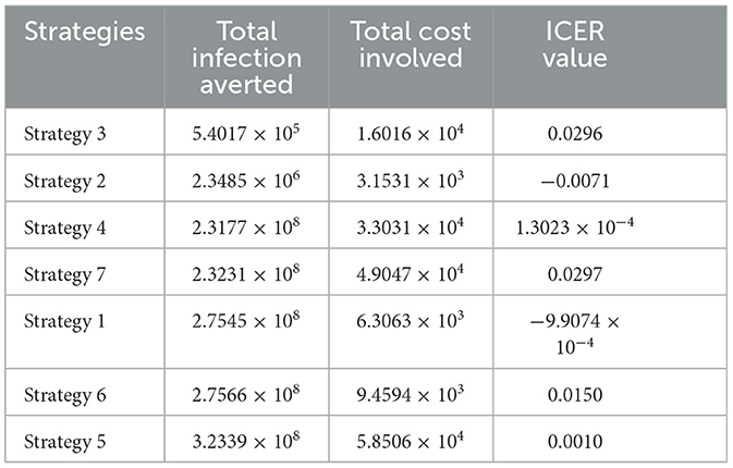
Table 3. Strategies' ICER values with their total infection averted and total cost involved.

Table 4

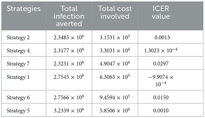
Table 4. Strategies' ICER values with their total infection averted and total cost involved.

Assessing strategy 2 and strategy 4 in Table 4, it is noticed from the ICER that strategy 2 is expensive to deploy in a resource-limited setting; hence, strategy 2 is removed from the list of possible controls, and the ICER is calculated again. This is presented in Table 5.

Table 5

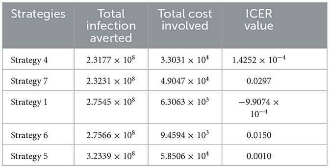
Table 5. Strategies' ICER values with their total infection averted and total cost involved.

Assessing strategy 4 and strategy 7 in Table 5, it is noticed from the ICER that strategy 7 is expensive to deploy in a resource-limited setting; hence, strategy 7 is removed from the list of possible controls, and the ICER is calculated again. This is presented in Table 6.

Table 6

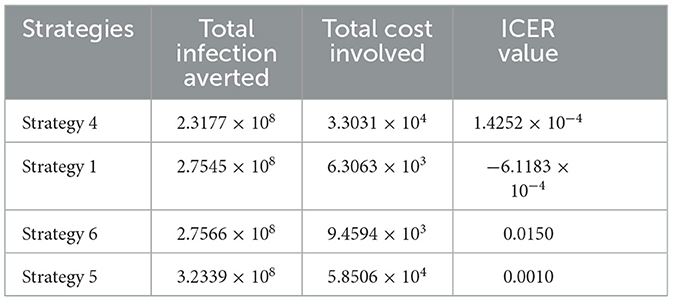
Table 6. Strategies' ICER values with their total infection averted and total cost involved.

Assessing strategy 4 and strategy 1 in Table 6, it is noticed from the ICER that strategy 4 is expensive to deploy in a resource-limited setting; hence, strategy 4 is removed from the list of possible controls, and the ICER is calculated again. This is presented in Table 7.

Table 7

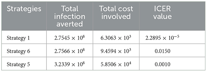
Table 7. Strategies' ICER values with their total infection averted and total cost involved.

Assessing strategy 1 and strategy 6 in Table 7, it is noticed from the ICER that strategy 6 is expensive to deploy in a resource-limited setting; hence, strategy 6 is removed from the list of possible controls, and the ICER is calculated again. This is presented in Table 8.

Table 8

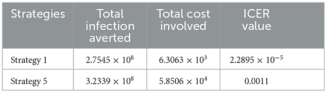
Table 8. Strategies' ICER values with their total infection averted and total cost involved.

Finally, assessing strategy 1 and strategy 5 in Table 8, it is noticed from the ICER that strategy 5 is expensive to deploy in a resource-limited setting; hence, strategy 5 is removed from the list of possible controls. Therefore, we conclude that strategy 1 is the most cost-effective strategy to use among the several strategies under study here. From the above analysis, it is obvious that strategy 1, thus, public education is the intervention that saves cost.

Conclusion

We have designed a new epidemiological co-infection vaccination model involving two strains of TB and COVID-19 to explore the transmission dynamics of tuberculosis (TB) and COVID-19 using data from Ghana. We have estimated the model's parameters and analyzed their effects on the two diseases' transmission through numerical and graphical illustrations. Again, we have exhibited the threshold dynamics of the basic reproduction number R₀ by evaluating the reproduction numbers of the two streams of the model, thus, TB and COVID-19 streams. It was found that the reproduction number of the TB stream with two strains: the drug-sensitive (DS) strain of TB, R_st = 0.55, and the reproduction number of the drug-resistant (DR) strain of TB, R_rt = 1.47. The reproduction number of the COVID-19 stream is R_0c = 2.21. This signifies that ~82.8% of TB and COVID-19 co-infection cases are drug-resistant (DR) strains of TB-induced, while 17.2% are drug-sensitive (DS) strains of TB-induced. The treatment of TB is not easy due to ineffective vaccines, as stated in [4, 5], which has also been demonstrated in this study. It was observed that the number of drug-resistant (DR) strains of TB and COVID-19 co-infection is higher in all cases (see Figures 5E–11E).

Our goal is to study the co-infection of tuberculosis (TB) and COVID-19 and devise strategies that save costs to mitigate the transmission; therefore, we have formulated optimal control strategies together with the cost-effectiveness analysis that consider control measures involving both pharmaceutical and non-pharmaceutical interventions to control TB and COVID-19 co-infection. We implemented the strategies (see Figures 5–11), and it was observed that public education and vaccination to prevent TB and COVID-19 should be intensified and reach ~25% of the population from the beginning and intensify in subsequent days. Vaccination should be enhanced up to ~25% of the population from the start and reach ~75% within 100 days of implementation, case holding, and case finding, as explained in [39], need ~75% enforcement within 100 days because they are helpful in controlling the spread of TB. This indicates that although vaccination is good, it largely depends on the rise of drug-resistant (DR) strain infections if treatment failure of individuals infectious with drug-sensitive (DS) strain occurs and also the inefficacy of vaccines. We therefore encourage the health service to enhance the mechanism for TB diagnosis by following the recommendation in [40] because it is difficult to treat TB.

It is also worth knowing that public education saves cost per the cost-effectiveness analysis compared to the other strategies raised in this study. This intervention can minimize TB and/or COVID-19, as illustrated in Figure 5. This intervention should reach about 25% of the population from the beginning and intensify up to 75% in the subsequent days to realize the results of strategy 1 (see Figure 5F). However, it is imperative to check the effectiveness and cost of all the strategies raised in this study when choosing a control measure.

The outcomes of the findings imply that both pharmaceutical and non-pharmaceutical measures are very important in controlling the transmission of TB and COVID-19 co-infection. These control measures should always be vigorous to create public awareness of TB and COVID-19, as illustrated in Figures 5F–11F, to reduce the effective contact rates and rates of acquiring TB and/or COVID-19, as illustrated in Figure 4. Pharmaceutical measures such as vaccination against TB and COVID-19 are important; however, they should be implemented with vigilance because of the existence of drug-resistant (DR) strains of TB; therefore, the control measure should be mild in the beginning, as illustrated in all the PRCCs of this study (see Figure 3).

Although we have demonstrated the co-infection dynamics of TB and COVID-19, this study is focused on the homogeneity of the population; we hope to extend this study to explore the transmission of TB and COVID-19 co-infection by considering the heterogeneity of the population, such as age and sex. We encourage the Ghana health service to be keen on observing the drug-resistant (DR) strain of TB since it has a higher infection rate compared to the drug-sensitive (DS) strain of TB, leading to a high co-infection rate of drug-resistant (DR) strain of TB and COVID-19 which is difficult to treat. In addition, individuals with TB and/or COVID-19 are encouraged to complete their prophylaxis, especially for TB, to help halt the transmission of TB and COVID-19.

Data availability statement

The original contributions presented in the study are included in the article/supplementary material, further inquiries can be directed to the corresponding authors.

Author contributions

RA: Conceptualization, Data curation, Formal analysis, Investigation, Methodology, Writing – original draft, Writing – review & editing. ZJ: Funding acquisition, Supervision, Writing – review & editing. JY: Formal analysis, Supervision, Writing – review & editing. JA: Formal analysis, Investigation, Writing – review & editing. YW: Formal analysis, Investigation, Validation, Writing – review & editing.

Funding

The author(s) declare financial support was received for the research, authorship, and/or publication of this article. This research was supported by National Natural Science Foundation of China grants 12231012, 61873154.

Conflict of interest

The authors declare that the research was conducted in the absence of any commercial or financial relationships that could be construed as a potential conflict of interest.

Publisher's note

All claims expressed in this article are solely those of the authors and do not necessarily represent those of their affiliated organizations, or those of the publisher, the editors and the reviewers. Any product that may be evaluated in this article, or claim that may be made by its manufacturer, is not guaranteed or endorsed by the publisher.

References

1. Adebisi YA, Agumage I, Sylvanus TD, Nawaila IJ, Ekwere WA, Nasiru M, et al. Burden of tuberculosis and challenges facing its eradication in West Africa. Int J Infect. (2019) 6:3. doi: 10.5812/iji.92250

PubMed Abstract | Crossref Full Text | Google Scholar

2. World Health Organization. World Health Statistics 2015. Geneva: World Health Organization (2015).

Google Scholar

3. World Health Organization. Global Tuberculosis Report 2016. Geneva: World Health Organization (2016).

Google Scholar

4. Chaulet P. Treatment of Tuberculosis: Case Holding Until Cure, WHO/TB/83. Geneva: World Health Organization (1983). p. 141.

Google Scholar

5. Reichman LB, Hersh Field ES. Tuberculosis: a Comprehensive International Approach, New York: Dekker. (2000).

Google Scholar

6. Chen Y, Wang Y, Fleming J, Yu Y, Gu Y, Liu C, et al. Active or latent tuberculosis increases susceptibility to COVID-19 and disease severity. MedRxiv. (2020). doi: 10.1101/2020.03.10.20033795

Crossref Full Text | Google Scholar

7. Salman AM, Ahmed I, Mohd MH, Jamiluddin MS, Dheyab MA. Scenario analysis of COVID-19 transmission dynamics in Malaysia with the possibility of reinfection and limited medical resources scenarios. Comput Biol Med. (2021) 133:104372. doi: 10.1016/j.compbiomed.2021.104372

PubMed Abstract | Crossref Full Text | Google Scholar

8. Zamir M, Nadeem F, Alqudah MA, Abdeljawad T. Future implications of COVID-19 through Mathematical modelling. Results Phys. (2022) 33:105097. doi: 10.1016/j.rinp.2021.105097

PubMed Abstract | Crossref Full Text | Google Scholar

9. Worldometers. Reported Cases and Deaths by Country or Territory. Available online at: https://www.worldometers.info/coronavirus/#countries (accessed April 30, 2022).

Google Scholar

10. Zegarra MAA, Infante SD, Carrasco DB, Liceaga DO. COVID-19 optimal vaccination policies: A modeling study on efficacy, natural and vaccine-induced immunity responses. Math Biosci. (2021) 337:108614. doi: 10.1016/j.mbs.2021.108614

PubMed Abstract | Crossref Full Text | Google Scholar

11. Alanagreh L, Alzoughool F, Atoum M. The human corona virus disease COVID-19: its origin, characteristics, and insights into potential drugs and its mechanisms. Pathogens. (2020) 9:331. doi: 10.3390/pathogens9050331

PubMed Abstract | Crossref Full Text | Google Scholar

12. Singh HP, Khullar V, Sharma M. Estimating the impact of COVID-19 outbreak on high risk age group population in India. Augment Human Res. (2020) 5:18. doi: 10.1007/s41133-020-00037-9

Crossref Full Text | Google Scholar

13. Lustig Y, Zuckerman N, Nemet I, Atari N, Kliker L, Regev-Yochay G, et al. Eurosurveillance | neutralizing capacity against delta (b.1.617.2) and other variants of concern following comirnaty (BNT162b2, BioNTech/pfizer) vaccination in health care workers, Israel. Euro Surveil. 26:2100557. doi: 10.2807/1560-7917.ES.2021.26.26.2100557

PubMed Abstract | Crossref Full Text | Google Scholar

14. Nasreen S, Chung H, He S, Brown K, Gubbay JB, Buchan SA, et al. Effectiveness of COVID-19 vaccines against variants of concern in Ontario, Canada. MedRxiv. doi: 10.1101/2021.06.28.21259420

Crossref Full Text | Google Scholar

15. Katella, Omicron K, Delta, Alpha, and More: What to Know About the Coronavirus Variants. (2022). Available online at: https://www.yalemedicine.org/news/covid-19-variants-of-concern-omicron (accessed 30 Apr, 2022).

Google Scholar

16. Bernal J, Gower AN, Gallagher CE. Effectiveness of COVID-19 vaccines against the b.1.617.2 (delta) variant. N Engl J Med. (2021) 385:585–594. doi: 10.1056/NEJMoa2108891

PubMed Abstract | Crossref Full Text | Google Scholar

17. Cherian S, Potdar V, Jadhav S, Yadav P, Gupta N, Das G, et al. Convergent evolution of SARS-CoV-2 spike mutations, l452r, e484q and p681r, in the second wave of COVID-19 in Maharashtra, India. BioRxiv. doi: 10.1101/2021.04.22.440932

PubMed Abstract | Crossref Full Text | Google Scholar

18. Takashita E, Kinoshita N, Yamayoshi S, Fujisaki S, Ito M, Chiba S, et al. Efficacy of antibodies and antiviral drugs against covid-19 omicron variant. N Engl J Med. 386:995–998. doi: 10.1056/NEJMc2119407

PubMed Abstract | Crossref Full Text | Google Scholar

19. Sarkar S, Khanna P, Singh AK. Impact of COVID- 19 in patients with concurrent co- infections: a systematic review and meta- analyses. J Med Virol. (2021) 93:2385–95. doi: 10.1002/jmv.26740

PubMed Abstract | Crossref Full Text | Google Scholar

20. Gao Y, Liu M, Chen Y, Shi S, Geng J, Tian J. Association between tuberculosis and COVID- 19 severity and mortality: a rapid systematic review and meta-analysis. J Med Virol. (2021) 93:194–6. doi: 10.1002/jmv.26311

PubMed Abstract | Crossref Full Text | Google Scholar

21. Tadolini M, García-García J-M, Blanc FX, Borisov S, Goletti D, Motta I, et al. On tuberculosis and COVID-19 co-infection. EurRespir J. (2020) 56:2002328. doi: 10.1183/13993003.02328-2020

PubMed Abstract | Crossref Full Text | Google Scholar

22. Visca D, Ong CWM, Tiberi S, Centis R, D'Ambrosio L, Chen B, et al. Tuberculosis and COVID- 19 interaction: a review of biological, clinical and public health effects. Pulmonology. (2021) 27:151–65. doi: 10.1016/j.pulmoe.2020.12.012

PubMed Abstract | Crossref Full Text | Google Scholar

23. Mousquer GT, Peres A, Fiegenbaum M. Pathology of TB/COVID- 19 co- infection: the phantom menace. Tuberculosis. (2021) 126:102020. doi: 10.1016/j.tube.2020.102020

PubMed Abstract | Crossref Full Text | Google Scholar

24. Yang H, Lu S. COVID- 19 and tuberculosis. J Transl Int Med. (2020) 8:59–65. doi: 10.2478/jtim-2020-0010

PubMed Abstract | Crossref Full Text | Google Scholar

25. van den Driessche P, James W. Reproduction numbers and sub-threshold endemic eqilibria for compartmental models of disease transmission. Math Biosci. (2002) 180:29–48. doi: 10.1016/S0025-5564(02)00108-6

PubMed Abstract | Crossref Full Text | Google Scholar

26. World Health Organization. Global Tuberculosis Report. In: Incidence of Tuberculosis (per 100,000 People) - Ghana | Data. Geneva: World Health Organization. Available online at: worldbank.org (2023).

Google Scholar

27. Our World in Data. COVID-19 cases. Available online at: https://ourworldindata.org/covid-cases (assessed 16 Dec, 2023).

Google Scholar

28. Li MY, Muldowney JS. Global stability for the seir model in epidemiology. Mathemat Biosci. (1995) 125:155–64. doi: 10.1016/0025-5564(95)92756-5

PubMed Abstract | Crossref Full Text | Google Scholar

29. Dontwi I, Obeng-Denteh W, Andam E. A mathematical model to predict the prevalence and transmissiondynamics of tuberculosis in Amansie West district, Ghana. Br J Mathemat Comp Sci. (2014) 4:402–25. doi: 10.9734/BJMCS/2014/4681

Crossref Full Text | Google Scholar

30. Tchoumi S, Diagne M, Rwezaura H, Tchuenche J. Malaria and COVID-19 co-dynamics: a mathematical model and optimal control. Appl Mathemat Model. (2021) 99:294e327. doi: 10.1016/j.apm.2021.06.016

PubMed Abstract | Crossref Full Text | Google Scholar

31. Omame A, Abbas M, Onyenegecha C. A fractional-order model for COVID-19 and tuberculosis co-infection using atanganaebaleanu derivative. Chaos, Solitons Fract. (2021) 153:111486. doi: 10.1016/j.chaos.2021.111486

PubMed Abstract | Crossref Full Text | Google Scholar

32. Rwezaura H, Diagne M, Omame A, de Espindola A, Tchuenche J. Mathematical modeling and optimal control of SARS-CoV-2 and tuberculosis co-infection: a case study of Indonesia. Model Earth Syst Environm. (2022) 8:5493e5520. doi: 10.1007/s40808-022-01430-6

PubMed Abstract | Crossref Full Text | Google Scholar

33. Khan MA, Atangana A. Mathematical modeling and analysis of COVID-19: a study of new variant omicron. Physica A. (2022) 599:127452. doi: 10.1016/j.physa.2022.127452

PubMed Abstract | Crossref Full Text | Google Scholar

34. WHO. Global tuberculosis Programme, treatment of tuberculosis: Guidelines for National Programmes (3rd ed.). (2020). Available online at: https://apps.who.int/iris/handle/10665/67890 (accessed January 12, 2024).

PubMed Abstract | Google Scholar

35. Osei E, Amu H, Kye-Duodu G, Kwabla MP, Danso E, Binka FN, et al. Impact of COVID-19 pandemic on Tuberculosis and HIV services in Ghana: An interrupted time series analysis. PLoS ONE. (2023) 18:e0291808. doi: 10.1371/journal.pone.0291808

PubMed Abstract | Crossref Full Text | Google Scholar

36. Asamoah JKK, Owusu MA, Jin Z, Oduro FT, Abidemi A, Gyasi EO. Global stability and cost-effectiveness analysis of COVID-19 considering the impact of the environment: using data from Ghana. Chaos, Solitons Fractals. (2020) 140:110103. doi: 10.1016/j.chaos.2020.110103

PubMed Abstract | Crossref Full Text | Google Scholar

37. Agusto F, Leite M. Optimal control and cost-effective analysis of the meningitis outbreak in Nigeria. Infect Dis Model. (2017) 4:161–87. doi: 10.1016/j.idm.2019.05.003

PubMed Abstract | Crossref Full Text | Google Scholar

38. Asamoah JKK, Okyere E, Abidemi A, Moore SE, Sun G, Jin Z, Acheampong E, Gordon JF. Optimal control and comprehensive cost-effectiveness analysis for COVID-19. Results Phys. (2022) 33:105177. doi: 10.1016/j.rinp.2022.105177

PubMed Abstract | Crossref Full Text | Google Scholar

39. Asamoah JKK, Jin Z, Sun G. Non-seasonal and seasonal relapse model for Q fever disease with comprehensive cost-effectiveness analysis. Results Phys. (2021) 22:103889. doi: 10.1016/j.rinp.2021.103889

Crossref Full Text | Google Scholar

40. CDC. Latent Tuberculosis Infection: A Guide for Primary Health Care Providers. Atlanta, GA: CDC (2014).

Google Scholar