Mathematical modelling of non-pharmaceutical interventions to control infectious diseases: application to COVID-19 in Kenya

Introduction: The first case of COVID-19 in Kenya was reported on March 13, 2020, prompting the collection of baseline data during the initial spread of the disease. Subsequently, the Kenyan government implemented non-pharmaceutical interventions (NPIs) on April 9, 2020, to mitigate disease transmission over a two-month period. These measures were later gradually relaxed starting from June 9, 2020.

Methods: We applied a deterministic mathematical model to simulate the dynamics of COVID-19 transmission in Kenya. Using baseline data, we estimated transmission and recovery rates and proposed a mathematical model of how NPIs affect disease transmission rates. The model extends to interventions that yield an increase in disease transmission, unlike previous models that were limited to a decrease in transmission. We computed the mitigation and relaxation fractions and hence deduced the impact of the interventions.

Results: The mitigation measures imposed from April 9, 2020, reduced the disease transmission by 43.7% from the baseline level, while the relaxation from June 9, 2020, increased the transmission by 32% over the mitigation level. Without intervention, the model predicts that infections would have peaked at 30% by late May 2020. However, due to the combined effect of mitigation and relaxation, the epidemic peaked at 13% infection in mid-July 2020.

Discussion: The model’s projections closely align with observed data, providing valuable insights for planning. Ongoing research aims to refine the model to capture sub-waves and spikes, as well as simulate multiple waves of infection. These efforts will enhance our understanding of COVID-19 dynamics and inform effective public health strategies. The estimated basic reproduction number ${\mathcal{R}}_0=2.76$ , consistent with previous findings, underscores the validity of our model and its relevance in predicting disease transmission dynamics.

1 Introduction

Coronavirus Disease of 2019 (COVID-19) is a disease caused by the novel coronavirus that appeared in Wuhan, China, in December 2019. The disease has since spread to all parts of the world and has resulted in millions of confirmed cases and deaths (1). The disease has wreaked havoc on the economies of most countries and permanently transformed people’s lives. To control the spread of disease, in the initial stages, countries introduced non-pharmaceutical interventions (NPIs) in addition to strengthening health facilities and treatment regimes. As time passed, the disease developed into waves that were mainly driven by variants of COVID-19.

We briefly present pertinent biological information on COVID-19 and a related disease, influenza, popularly known as flu. Our reference to influenza here will mean seasonal and not pandemic influenza. In the early days of COVID-19, many people confused the disease with the flu, since both show almost identical symptoms. On 11th February 2020, the virus that causes COVID-19 was named ‘severe acute respiratory syndrome coronavirus 2 (SARS-CoV-2)’ by the International Committee on Taxonomy of Viruses (ICTV) (2). The flu is caused by influenza viruses types A, B, and C. Influenza and SARS-CoV-2 are spread through droplets released from the nose and mouth of an infected individual when they cough or sneeze (3). However, unlike influenza, COVID-19 has also been shown to spread by the long-range airborne route at greater distances (4). A critical determinant of the infectivity of these viruses is the concept of reproduction number ${\mathcal{R}}_0$ , which represents the degree of transmissibility of the virus and provides an estimate of how many secondary infections can arise from one person infected with the virus, in a population where everyone is susceptible to the disease. In the early stages of the epidemic, the ${\mathcal{R}}_0$ for COVID-19 was estimated to be 2.2–2.5 (5). Since then, most of the published estimates for ${\mathcal{R}}_0$ lie in the range 2–3. For seasonal influenza, studies yielded ${\mathcal{R}}_0$ in the range of 1.1–1.5 (6), suggesting that COVID-19 is more easily spread than seasonal influenza. For both flu and COVID-19, it is possible to spread the virus at least 1 day before experiencing any symptoms. Once an individual has the flu, the person can be contagious for 5 to 7 days, while for COVID-19 the person could be contagious for 10 to 14 days. The number of days of staying contagious will depend on the patient’s age, the severity of the disease and whether there are other underlying medical conditions (7, 8). Mortality from COVID-19 is believed to be much higher than that of seasonal influenza (8, 9).

Mathematical models can be used to inform and provide health decisions during a disease outbreak; in addition, they can be used to predict and perform the peak detection of infected cases in a particular country. Various mathematical models have been applied to understand the dynamics of COVID-19, as can be seen from a recent extensive review (10). In this study, we consider the compartmental model, where the population is usually divided into various compartments such as Susceptible (S), Exposed (E), Infected (I), Recovered (R), and Dead (D). If all compartments are included, then the model is said to be SEIRD. Models do not necessarily use all compartments, and in our case, we omit the exposed compartment and hence end up with the SIRD model, which has been used before for COVID-19; see, for instance, (11–13). Irrespective of the number of compartments used, models can be modified to include additional compartments such as asymptomatic, hospitalized, and vaccinated, among others (14–16).

In addition to mathematical models for the analysis of COVID-19 dynamics, some models address non-pharmaceutical interventions (NPIs) designed to control the spread of the disease. As a starting point for these models, it is important to have an understanding of the baseline dynamics and, hence, estimates of the parameters associated with the unmitigated disease, since they are essential to the implementation of interventions. Two of these parameters are particularly useful, namely, the transmission rate, β(t), which is the number of contacts per person per unit of time, and the basic reproduction number, ${\mathcal{R}}_0$ . In most situations, intervention starts almost immediately as COVID-19 emerges and baseline parameters are estimated later, using data collected from the period preceding any major mitigation measures. The main purpose of the intervention is to reduce the contact rate and hence the reproduction number, so that the peak of infection reaches a level that can be managed by available healthcare facilities and personnel.

The mathematical models we consider here are based on the SEIRD formulation, with one or two compartments omitted in some cases. The models can generally be classified into two categories. In the first category, there are models in which additional compartments are introduced into the SEIRD system that have an impact on NPIs, for example, control interventions (17), masks and their efficiency (18), and hospitalization (19), among others. In the process, they introduce more parameters that define how the additional compartments interact with each other and with the rest of the system. The consequence is that the system of differential equations becomes more complex and the number of parameters to be estimated increases significantly. In the second category of models, the intervention measures are collectively deemed to reduce the transmission rate from the time the intervention occurs. The reduction can be reflected in several ways. In the simplest case, the constant transmission rate, before intervention, is multiplied by a positive constant, which is less than unity, to obtain a reduced transmission rate (20). The transmission rate can also be specified as a piecewise constant function, depending on the mitigation measures enforced (21), or as an exponentially decaying function (13, 22). In this category of models, the system of equations is less complicated. Furthermore, recovery and death rates are assumed to remain constant, except for a formulation in which they are time-dependent (13). In this paper, we use the methods in the second category since they are flexible and can easily be applied to develop scenarios. We express the transmission rate as a function that can exponentially decay, thus reducing the level of infection, or exponentially increase, thus increasing the level of infection, as formulated in (23). Previous models were able to handle only a decrease in infection level.

The overall aim of this study is to approximate the SIRD model parameters using COVID-19 data from the baseline period in Kenya and thereafter introduce a mathematical model that illustrates how NPIs collectively affect the transmission rate of COVID-19 and hence infection levels. The model was applied to the first wave of COVID-19 in Kenya, since this was the period in which NPIs were implemented and properly documented. For the subsequent waves that emerged after the study period, the dynamics of the disease was largely influenced by the new variants of COVID-19 and the vaccinations that emerged from time to time. This study therefore forms a starting point of coupling the PIs and NPIs to faithfully describe the emergence of multiple waves of COVID-19 and other related diseases like Flu.

The rest of the paper is organized as follows. In Section 2.1, we briefly describe the COVID-19 situation in Kenya and present the major NPIs and the timelines in which they were proposed. In Section 2.2, the SIRD model equations and initial conditions are given. A description is given in Section 2.3 of a mathematical model for interventions that takes into account the fact that interventions lead to a reduction of the transmission rate, in the case of mitigation, or an increase in the transmission rate, when some mitigation measures are lifted or when the society violates prescribed mitigation regulations. In Section 3.1 we present the solution of the SIRD model for the baseline. Section 3.2 presents the results of the interventions. Finally, we give some concluding remarks and recommendations in Section 4.

2 Methods

2.1 COVID-19 in Kenya

The rapidly spreading outbreak of the novel coronavirus on the African continent prompted the Kenyan government to establish the National Emergency Response Committee on Coronavirus (NERC) on 28 February 2020. Approximately 2 weeks later, the first case of COVID-19 in Kenya was confirmed on 13 March 2020 (24). Due to the rapid increase in cases, the Kenyan government instituted several measures designed to curb the spread of the disease. For our modelling, the strategies pursued can be divided into four periods, each with its distinct characteristics as outlined below and also shown in Table 1.

Table 1

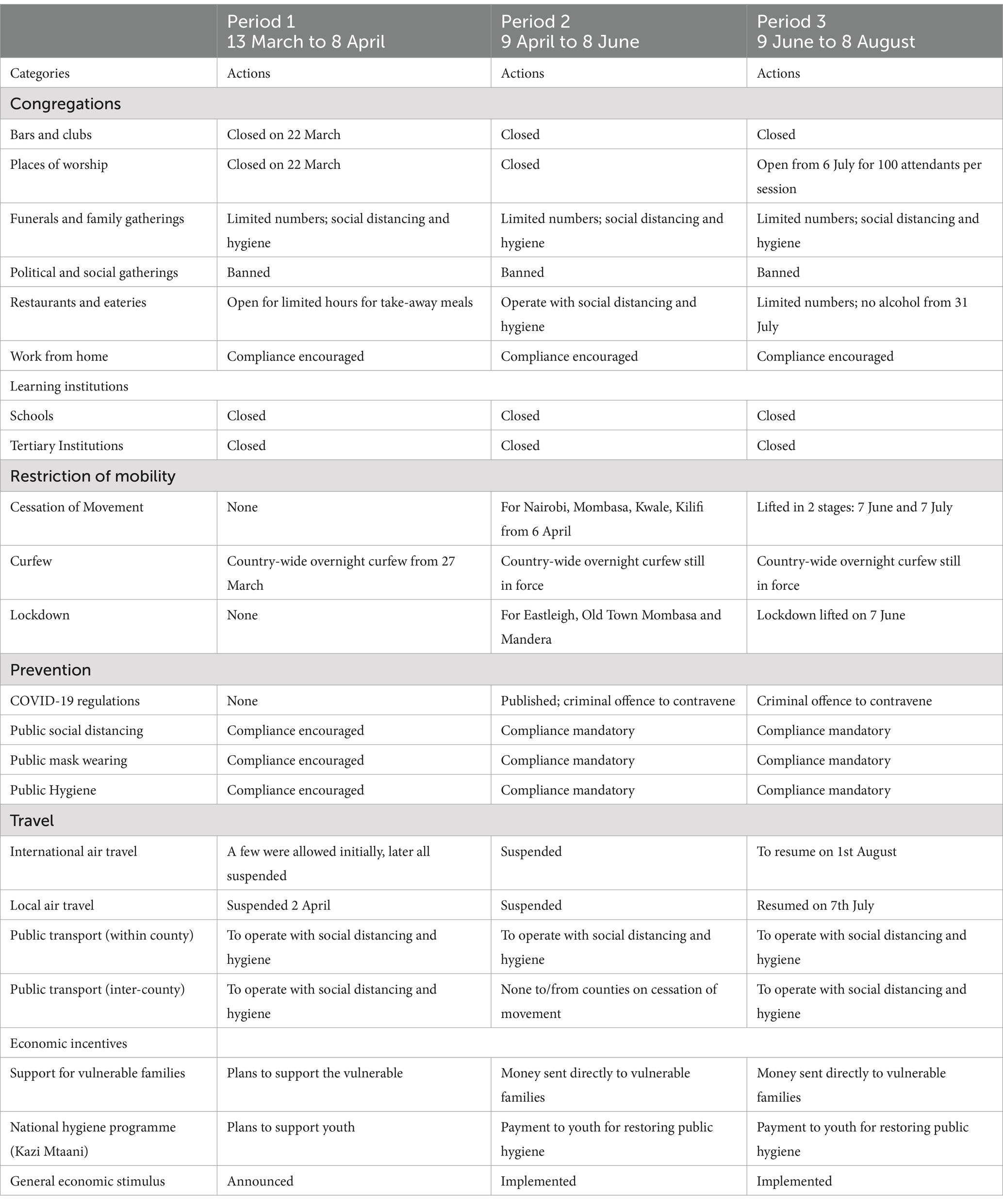
Table 1. Strategies for mitigating COVID-19 in Kenya in 2020.

2.1.1 Period 1: Baseline (13 March to 8 April)

Since COVID-19 was a novel disease, this period was spent formulating policies and protocols on how to respond to it. A major decision was to immediately close the learning institutions. Other mitigation measures were announced, for instance: no overcrowding in public transport; social distancing and mask-wearing in public places; hand-washing and sanitization in malls and supermarkets. There was low compliance, so a lot of time was spent appealing to residents to comply with the measures. In anticipation of the potential impact of the pandemic, the government introduced a tax break to provide some relief to residents. Despite the mitigation measures enacted, it was business as usual in most places. This period can, therefore, be safely regarded as the time when COVID-19 was still unmitigated. Hence, our model treats this period as the baseline.

2.1.2 Period 2: Mitigation (9 April to 8 June)

Due to the rapid increase in cases, and the public’s relaxed attitude to COVID-19, the government resolved to enforce the mitigation measures for 2 months and it enacted COVID-19 regulations whose contravention was a criminal offence (25, 26). The period can be regarded as one of the applications of mitigation measures, despite attempts by a cross-section of society to flout the rules. Consequently, our model treats this as a mitigation period.

2.1.3 Period 3: Relaxation (9 June to 8 August)

The implementation of mitigation measures during Period 2 had a devastating effect on the country’s economy and the livelihoods of the people. Many industries and small businesses laid off workers or simply folded. Other establishments placed workers on half salary or gave them leave without pay while waiting for the situation to stabilize. To ease the hardship being experienced, the government gradually relaxed some of the mitigation measures. There was a discussion on the opening of learning institutions in September, but the idea was shelved on the basis of the pandemic trend. Our model treats this period as the gradual relaxation of control measures.

2.1.4 Period 4: Extended Relaxation (9 August 2020 to 30 September)

No significant changes were made to the relaxation measures that were supposed to be in effect during Period 3. Consequently, we treated these measures as remaining in effect until the appearance of the second wave of COVID-19 in September 2020. We thus regarded this as a period of extended relaxation.

Table 1, gives a summary of the major actions taken during each of the first three periods. The information in this table was obtained from the Ministry of Health, Kenya (25) and the Presidential Addresses on COVID-19 (27).

Figure 1 shows the trend of the 7-day moving averages of numbers and percentages of infections, deaths, and recoveries, from 25th March 2020 to 20th October 2020.

Figure 1

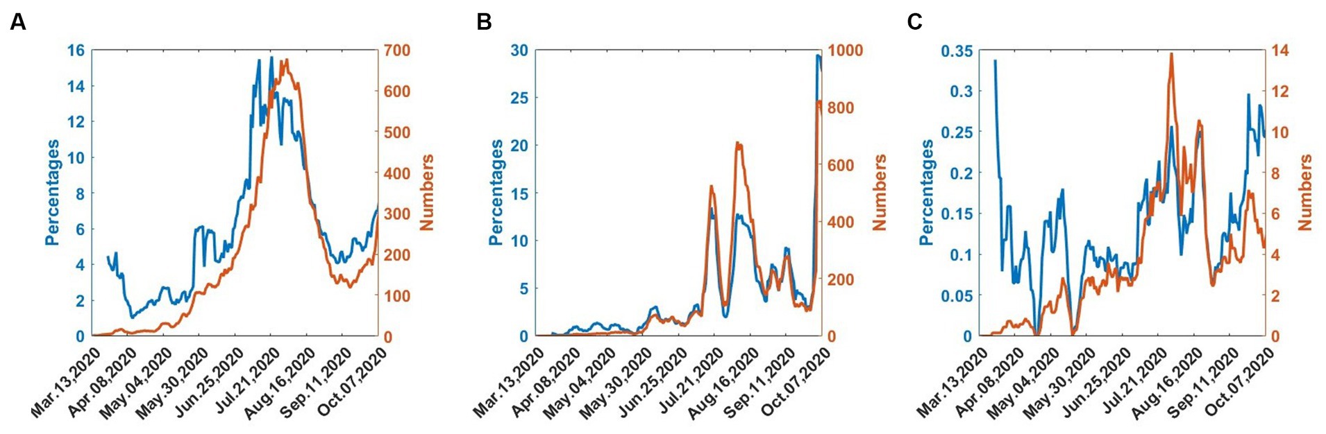
Figure 1. COVID-19 numbers and percentages from 25th March 2020 to 30th September 2020. (A) Infected. (B) Recovered. (C) Dead.

In Figure 1A, the infections gradually increase and reach a maximum in mid-July. The infections then decrease until early September, when they begin to increase, indicating the onset of the second wave. In Figure 1B, the recoveries also follow the wave pattern of the infections but there exist considerable fluctuations. Figure 1C shows that deaths exhibit considerable fluctuations but the numbers are generally low.

2.2 Formulation of the SIRD model for COVID-19

We consider an SIRD mathematical model. We assume homogeneous mixing in the population and that the total population, N, is constant over time. At time t, the number of individuals in the population is divided into four classes: Susceptible, S_N(t), infected, I_N(t), recovered, R_N(t), and dead, D_N(t). Since this is a new disease, there is no prior immunity; hence at the beginning, everyone is susceptible to COVID-19. As the total population, N, is constant over time, the numbers of individuals in the various compartments satisfy the equation.

$\begin{array}{ll}{S}_N\left(t\right)+I_N\left(t\right)+R_N\left(t\right)+D_N\left(t\right)=N& (1)\end{array}$

If the variables are normalized on division by N, then Equation (1) becomes

$\begin{array}{ll}\mathrm{S}\left(\mathrm{t}\right)+\mathrm{I}\left(\mathrm{t}\right)+\mathrm{R}\left(\mathrm{t}\right)+\mathrm{D}\left(\mathrm{t}\right)=1& (2)\end{array}$

where

$\begin{array}{ll}S=S_N/N,I=I_N/N,R=R_N/NandD=D_N/N& (3)\end{array}$

in which S, I, R and D are fractions of susceptible, infected, recovered, and dead individuals, respectively. Upon infected with the disease, susceptible individuals move to the infected class at a rate β, from which they recover at a rate γ or die from infection at a rate δ, as shown in Figure 2. In the presentation of our results, the variables will be given as convenient in terms of actual observed numbers or percentages or as fractions of the total population.

Figure 2

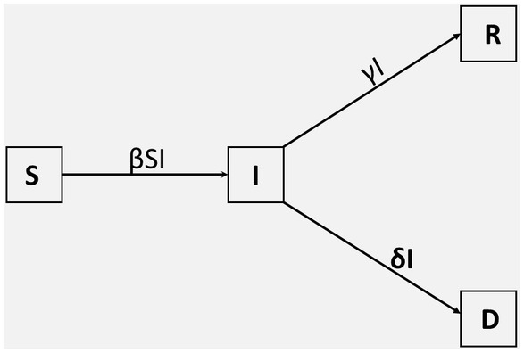
Figure 2. Compartmental SIRD model. The population is divided into four classes, denoted by; S(t), I(t), R(t), and D(t). The parameters β, γ, and δ denote the transmission rate, the recovery rate, and the death rate, respectively.

The mathematical equations describing the movement of individuals in different compartments are given by;

$\begin{array}{ll}dS/dt=-\beta SI& (4)\end{array}$

$\begin{array}{ll}dI/dt=\beta SI-\left(\gamma +\delta \right)I& (4)\end{array}$

$\begin{array}{ll}dR/dt=\gamma I& (4)\end{array}$

$\begin{array}{ll}dD/dt=\delta I& (4)\end{array}$

These equations are solved subject to Equation (2) and also subject to non-negative initial conditions: S(0), I(0), R(0), and D(0). The SIRD model has already been applied to COVID-19 (11–13) and seasonal influenza (28–30).

2.3 Modelling interventions

In this section, we first derive the equations that define the effect of interventions on the disease transmission rate. We then indicate how intervention scenarios can be developed to help in decision-making and, finally, we indicate how the appropriate intervention model can be identified amongst the many possible scenarios.

2.3.1 Equations governing the effect of intervention on the transmission rate

In this subsection, we formulate an intervention model that leads to piecewise exponential-cum-constant functions for the transmission rate. We assume that the recovery rate, $\gamma$ , and the death rate, δ, do not change during the intervention interval. Our model takes into account the fact that intervention not only leads to a reduction of the transmission rate, through mitigation but can lead to a surge in the transmission rate, through relaxation.

Let the daily intervention events be at the time nodes denoted as $t_0,t_1,t_2,\dots$ . Suppose intervention is initiated at the time node $t_k$ then there will be a difference in the transmission rate before and after $t_k$ . Let β_b be the incoming transmission rate before and up to, the time $t_k$ ; the quantity β_b could be the result of baseline dynamics or it could be due to the dynamics from some immediately preceding intervention. The main objective of intervention is to gradually change the transmission rate from β_b, by a fraction c, so that the transmission rate at a future time becomes.

$\begin{array}{ll}{\beta }_{op}=\beta \left(t_{k+m}\right)=\left(1-c\right){\beta }_b& (5)\end{array}$

where ${\beta }_{op}$denotes the optimum value of the transmission rate that is achieved due to the intervention at time $t_k$ . When an intervention takes place on day $t_k$ , the optimum transformation of the transmission rate does not occur instantly but takes place say m days later, that is, at the time $t_{k+m}$ , where m > 0. Therefore, the quantity m can be regarded as the duration of an optimal change in transmission rate and its value will depend on the implementation goals. For instance, when we impose measures to reduce social distancing, we do not expect infection levels to drop instantly; it takes 7 to 20 days to show a significant change.

From Equation (5), when 0 < c < 1, then β_op < β_b; this corresponds to the intervention being mitigation since it yields a smaller future transmission rate, in which the incoming transmission rate has been reduced by a fraction c. Here, we call c the “mitigation fraction” and the quantity ${\left(100c\right)}^{\%}$ the “percent mitigation.” On the other hand, when c < 0 then β_op > β_b; this corresponds to the intervention being a relaxation since it produces a higher future transmission rate in which the incoming transmission rate has been increased by a fraction $\left|c\right|$ . Here we call $\left|c\right|$ the “relaxation fraction” and the quantity $\left(100\left|c\right|\right)\%$ the “percent relaxation.” Previous researchers restricted c to the interval [0, 1]; consequently, they could only handle the cases where intervention resulted in a decrease in the transmission rate. In this presentation, we extend c to negative values to account for an increase in the transmission rate.

Assume that the impact of the intervention at $t_k$ results in a transmission rate, β(t), which changes exponentially for $t_k>0$ , that is,

$\begin{array}{ll}\beta \left(t\right)=A{e}^{r\left(t-t_k\right)},\mathrm{}t\ge t_k& (6)\end{array}$

where A and r are constants to be determined.

To determine the constants A and r in Equation (6), we impose the conditions

$\begin{array}{ll}\beta \left(t_k\right)={\beta }_b\mathrm{};\mathrm{}\beta \left(t_{k+m}\right)=\left(1-c\right){\beta }_b& (7)\end{array}$

We assume that when ${\beta }_{op}$ , in Equation (5), is reached the transmission rate remains constant until another intervention takes place at the time $\tau >t_{k+m}$ . Consequently, applying Conditions (7) to Equation (6) yields the expression for the transmission rate in the following form, as given in Supplementary Appendix Equations (A9, A10):

$\beta \left(t\right)=\{\begin{array}{c}{\beta }_b,\mathrm{}\mathrm{}\mathrm{}\mathrm{}t\le t_k\\ {\beta }_b{e}^{g\left(t\right)},\mathrm{}\mathrm{}{t}_k\le t\le t_{k+m}\\ {\beta }_{op}=\left(1-c\right){\beta }_b,\mathrm{}{t}_{k+m}\le t<\tau \end{array}\mathrm{}\text{ (8)}$

where

$\begin{array}{ll}g\left(t\right)=\left[\frac{\left(t-t_k\right)\ln \left(1-c\right)}{t_{k+m}-t_k}\right]& (9)\end{array}$

If we substitute $t=t_{k+m}$ in the second part of Equation (8), we obtain $\beta \left(t_{k+m}\right)=\left(1-c\right){\beta }_b$ , consistent with Equation (5). We can analyze the intervention that takes place at τ by letting $\mathrm{\tau }=t_k$ and proceeding as is done in the current section. This allows us to treat multiple interventions until there are no more interventions. We have shown in Supplementary Appendix A that, in the absence of further interventions, the transmission rate will decay with time, if the last intervention is a mitigation, or grow without bounds, if the last intervention is a relaxation. Therefore, for practical considerations, the last intervention must be a mitigation.

Associated with the transmission rate, β, is the basic reproduction number, ${\mathcal{R}}_0$ , which denotes the average number of secondary infections directly generated by an infected individual in a population where all individuals are susceptible to infection. It is given by

$\begin{array}{ll}{\mathcal{R}}_0=\frac{\beta }{\gamma +\delta }& (10)\end{array}$

where γ and δ are the rates of recovery or death from the disease, respectively, as indicated in Figure 2. If ${\mathcal{R}}_0>1$ the disease will expand and if ${\mathcal{R}}_0<1$ , the disease will die out. A related quantity is the effective reproduction number, ${\mathcal{R}}_e$ , given by

$\begin{array}{ll}{\mathcal{R}}_e=\frac{\beta \left(t\right)S\left(t\right)}{\gamma +\delta }& (11)\end{array}$

in which S(t) is the proportion of susceptible individuals at time t. The effective reproduction number, Equation (11) defines the potential for an epidemic to spread as a result of the interventions put in place. If ${\mathcal{R}}_e>1$ , the epidemic will spread at time t, and if ${\mathcal{R}}_e<1$then the epidemic will not spread at time t.

2.3.2 Estimation of mitigation and relaxation fractions

Despite the importance of the intervention fraction, c, only two of its values are obvious, namely, c = 0 which implies the absence of any control, and c = 1, which is the unlikely scenario of absolute control where there is no disease transmission. The other values of c are more complicated to determine. A possible approach is to identify all interventions that impact the transmission of the disease, therefore contributing to c, and assign weights to their impacts. The fraction c can then be estimated as the weighted average of the impacts. Groups of the impacts could then be aggregated to determine their percentage contribution to the disease transmission. Table 1 lists some intervention measures that could be taken into account in this exercise. Assessing the impact of all these factors on disease transmission requires a truly collaborative effort involving a multidisciplinary team.

2.3.3 Intervention scenarios

Mitigation is the first intervention that takes place after the baseline dynamics; hence, it is assumed that the equations in Section 2.2 have been solved and the appropriate baseline parameters obtained. Consequently, the incoming transmission rate for the mitigation intervention will be the transmission rate from the baseline solution. Relaxation occurs when mitigation ends, and hence it is assumed that the mitigation problem has been solved so that the transmission rate during mitigation can be used as the incoming transmission rate for relaxation computations.

Starting with the appropriate incoming transmission rate, we may vary the fraction c, in Equations (8, 9), as we solve Equations (4a-d), and thus determine the effect of an intervention on the transmission rate, infection levels, reproduction number, and related quantities. It enables us to develop scenarios as we seek to determine the levels of intervention necessary to achieve specific medical and public health goals as a consequence of the pandemic. The scenarios can form a basis for decision-making. For instance, modellers using different techniques developed two intervention scenarios for the control of COVID-19 in some African countries (31). The first was moderate lockdown, considered as the intervention that reduces transmission by 25% during lockdown followed by transmission at 90% of the pre-lockdown value. The second was hard lockdown, considered as the intervention that reduces transmission by 44% during lockdown followed by transmission at 90% of the pre-lockdown value. In our formulation, moderate lockdown is equivalent to mitigation with c = 0.25 followed by relaxation with c = −2.6 while hard lockdown is equivalent to mitigation with c = 0.44 followed by relaxation with c = −1.05.

2.3.4 Model validation

Once infection data is available, the computation can be carried out as described in Section 2.3.3, to determine the model infection curve that best fits the data. The objective of this section is to validate the model and not to develop scenarios. The simplest approach is to draw a scatter diagram of observed infections and plot it against infection curves obtained by using different values of the mitigation or relaxation fractions, c, as appropriate. We then identify the value of c for which the curve closely matches the observed data. This value of c will be an indicator of the fraction by which the infection has changed, as a result of the intervention. It can be used, through Equations (8, 9), in our solution of Equations (4a-d), to obtain other vital information. This scatter diagram approach will yield coarse estimates. More robust and reliable methods are based on techniques that minimize errors between observed and computed infection rates using a variety of approaches. The parameters, $\beta$ , $\gamma$ and c were estimated by formulating a least-squares algorithm, to minimize the distance between the daily and cumulative infected numbers to the model output. The least-squares algorithm was solved in MATLAB using the fminsearchbnd function, which allows for parameter estimation from a range of bounded parameters (32). We consider the root mean square error, defined by Equation (12), as the objective function to be minimized.

$\begin{array}{ll}\tilde{R}\left(\gamma \mathrm{,}\beta \right)=RMSE\left(I\right)=\sqrt{\frac{{\displaystyle \sum }_{k=1}^{k_M}{\left(I_k^c-I_k^o\right)}^2}{k_M}}& (12)\end{array}$

in which RMSE stands for the root mean square error; $I_k^{c}and{I}_k^o$are the observed and computed infection proportions, respectively, at the time $t_k$ ; and $k_M$ is the total number of continuous-time steps of observations during the period under consideration. This model validation process can be performed at any stage in data collection, and it does not need to wait until the end of the designated intervention period.

3 Results and discussion

We developed models and performed computation using MATLAB, according to the timelines specified in Section 2.1. We first present results for solutions of the SIRD system using the method described in Section 2.2; then we present results for the intervention model described in Section 2.3. COVID-19 data were obtained from the following sources: Worldometer (1) and Ministry of Health, Kenya (25).

3.1 Solution of SIRD system for the baseline period

The first infected person was observed and tested on 13th March 2020 and by the end of the baseline period, namely 8th April 2020, a total of 5,586 individuals had been tested. If the entire population of Kenya had been tested by 8th April 2020, the number of infected individuals would have increased, but in such a way that the proportion of infected individuals for the whole country would be equal to the proportion of infected individuals in the sample of 5,586. Similar arguments can be made for individuals in the susceptible, recovered, and dead compartments. Since the proportions of the various compartments remain the same, irrespective of the sample size tested by 8th April 2020, we can take the total population during the baseline as N = 5,586.

At the start of the epidemic, there was one infected individual, that is, I_N(0) = 1. At this stage, there were no recoveries or deaths, which implies that R_N(0) = D_N(0) = 0, leading to S_N(0) = 5,585, according to Equation (1). Using Equation (3) we obtain the initial conditions.

$\mathrm{I}\left(0\right)=1.79018976\mathrm{E}-04,\mathrm{R}\left(0\right)=0,\mathrm{D}\left(0\right)=0,\mathrm{S}\left(0\right)=0.999820981$

The death rate was taken as $\delta =0.015$ , as estimated from the case fatality rate (CFR). The solution of Equations (4a-d) was then obtained, as described in Section 2.2, subject to the initial conditions (13) and also to Equation (2), at any time t.

The solution by minimization in MATLAB yielded the following parameter values:

$\begin{array}{ll}\beta =0.189919,\gamma =0.053811& (13)\end{array}$

From these results, we determined the reproduction number by Equation (10) and the recovery days, namely, 1/γ, to yield

$\begin{array}{ll}{\mathcal{R}}_0=2.76,& (14)\end{array}$

Recovery days (1/γ) = 18.6

The reproduction number and recovery days in Equation (14) are in good agreement with the results of other research (31).

Using the parameter values in Equation (13), with δ = 0.015, to solve system (4), we plotted graphs of some quantities. Figure 3A shows the 7-day moving average of the observed and computed infection percentages and numbers during the baseline period. Figure 3B shows the observed and computed cumulative infection percentages and numbers. In both figures, the agreement is good between the computed and observed values.

Figure 3

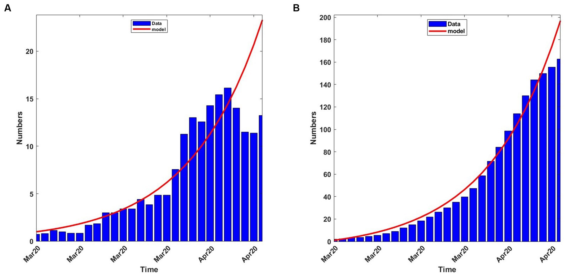
Figure 3. Observed and computed infection percentages during the baseline period, 13th March 2020 to 8th April 2020. For the model: Transmission rate, β = 0.188919; recovery rate, γ = 0.053811; death rate, δ = 0.015. (A) 7-day average percentages and numbers. (B) Cumulative percentages and numbers.

The system of equations was also solved from the onset until stability was achieved, thus assuming that the disease spread without any intervention. The results are shown in Figure 4 which indicates that the disease would have peaked in mid-June 2020, with 26 to 28% of the population infected. The graph also shows that the disease, without intervention, would have disappeared virtually by mid-October 2020. The decision to introduce mitigation measures was largely driven by the prospect of a quarter of the population being infected, at the peak of infection, and the possible adverse social and economic consequences.

Figure 4

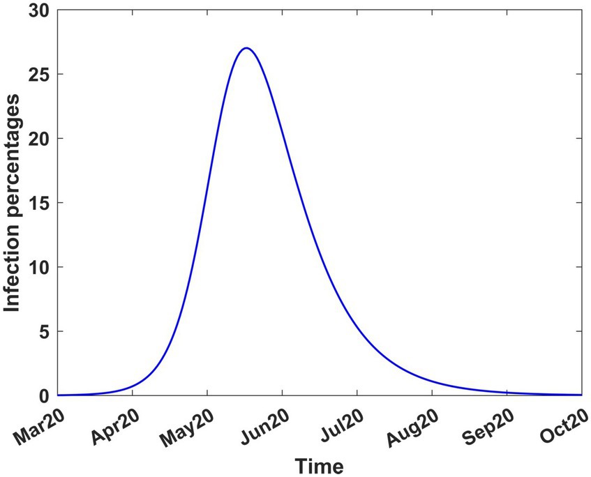
Figure 4. COVID-19 infection percentages in Kenya in the absence of interventions. The solution extends to stability. Transmission rate, β = 0.189919; recovery rate, γ = 0.053811; death rate, δ = 0.015.

3.2 Results from modelling interventions

In this section, we give results from intervention modelling, that show how the mitigation measures that were introduced on 9th April 2020 altered the dynamics of the disease. We use the parameter values in Equation (13), with δ = 0.015, and the methods in Sections 2.3.3 and 2.3.4 to solve the intervention problems. We present the mitigation results in Section 3.2.1 and the relaxation results in Section 3.2.2.

3.2.1 Mitigation from 9th April 2020 to 8th June 2020

Mitigation was introduced on 9th April 2020 for a period of 2 months (Table 1). To study the effect of different mitigation strategies, we developed scenarios by varying the fraction c in the transmission rate in Equations (8–9). We took into account the fact that the Kenyan government had received advice from modellers to take action on mitigation measures, considering scenarios involving a reduction in transmission by 20, 40, and 60% from the baseline (27). To extend the scope of scenarios, we added three more percentages and thus considered the consequence of reducing the transmission by 0% (c = 0, no change), 10% (c = 0.1), 20% (c = 0.2), 40% (c = 0.4), 60% (c = 0.6) and 80% (c = 0.8). We chose the incoming transmission rate at the start of mitigation as the baseline transmission rate (Equation 13), hence β_b = 0.189919. Using this value and m = 15 in Equations (8, 9), we solved system (4) from 9th April 2020 to stability. Figure 5 shows the infection curves associated with different values of c. Each curve shows the trajectory of the infection as a result of one-time mitigation on 9th April 2020, without subsequent interventions. It can be seen that as the value of c increases, the infection peaks reduce and occur later, meaning that the more stringent the mitigation measures, the lower the peak infections and they appear at a later time.

Figure 5

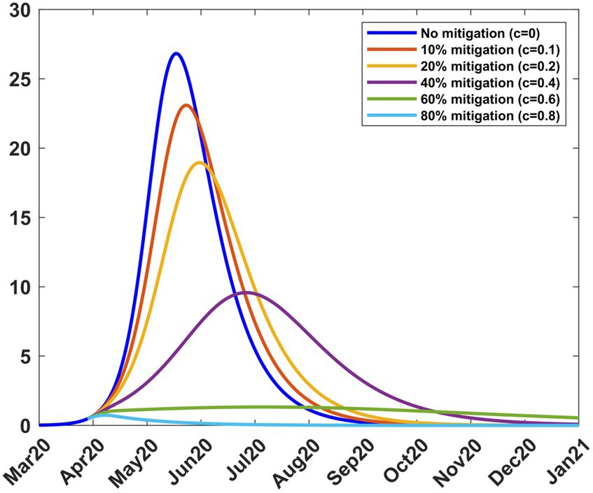
Figure 5. Infection percentages for various mitigation scenarios. Mitigation started on 9th April 2020. Solutions extend to stability. Incoming transmission rate, β_b = 0.189919; recovery rate, γ = 0.053811; death rate, δ = 0.015.

Table 2 shows how varying c affects the transmission rate, the reproduction number, and the infection. It is noted that as c increases, the peak infection and the reproduction number decrease. Further increase shows that for c = 0.8, the peak infection is 0.71% and ${\mathcal{R}}_0$ =0.55 < 1, meaning that there is no spread of the disease. This situation represents taking a mitigation action that is so drastic that the disease is suppressed; the consequences for such action can be severe for society. Therefore, suppression of the disease is not a practical option. Table 2 also shows the infection at the end of the mitigation period, namely, 8th June 2020. The model thus enables the planner to forecast, on 9th April 2020, the level of infection when mitigation ends.

Table 2

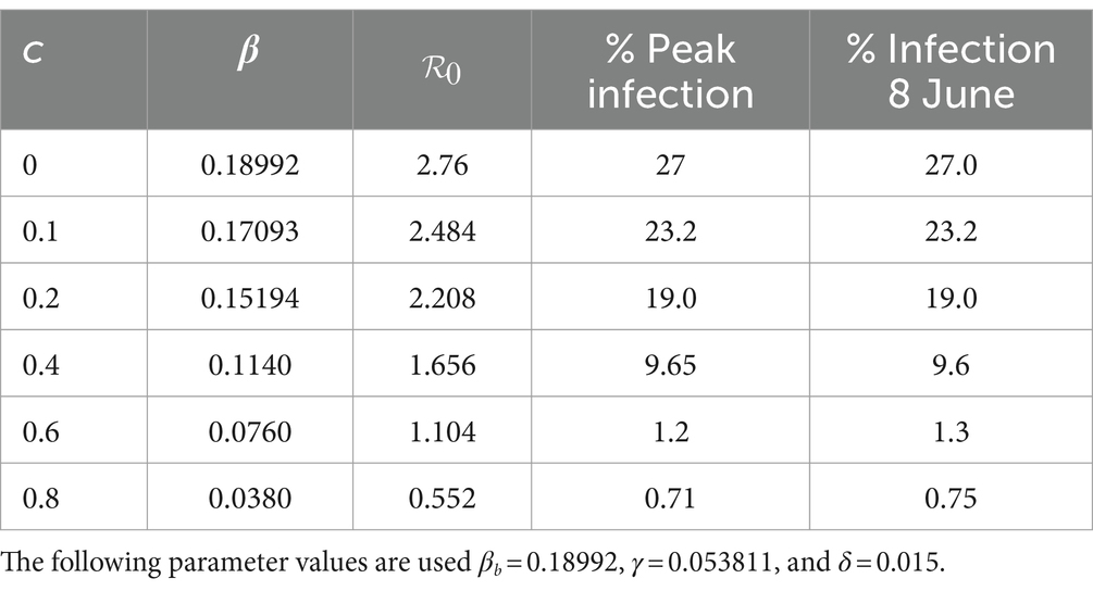
Table 2. Scenarios involving changes in the fraction c under mitigation from baseline.

To validate the model, we applied the methods in Section 2.3.4 to the mitigation data and obtained a mitigation fraction of c = 0.437. The result shows that the mitigation measures introduced by the government led to a reduction of the transmission rate by 43.7%, from that during the baseline (Equation 13) so that the optimum transmission rate during mitigation becomes β_t = 0.10692. The percentage reduction achieved is close to one of the scenarios, namely 40%, that the government had been advised to choose (27). The use of c = 0.437, m = 15 and β_b = 0.189919 in Equations (8, 9) and subsequent solution of system (4) produced results that are compared to the data in Figure 6A. There was some scatter in the data, largely attributed to the uncertainty in handling COVID-19 data during the early stage of the pandemic. This affected the quality of agreement of the model with the data.

Figure 6

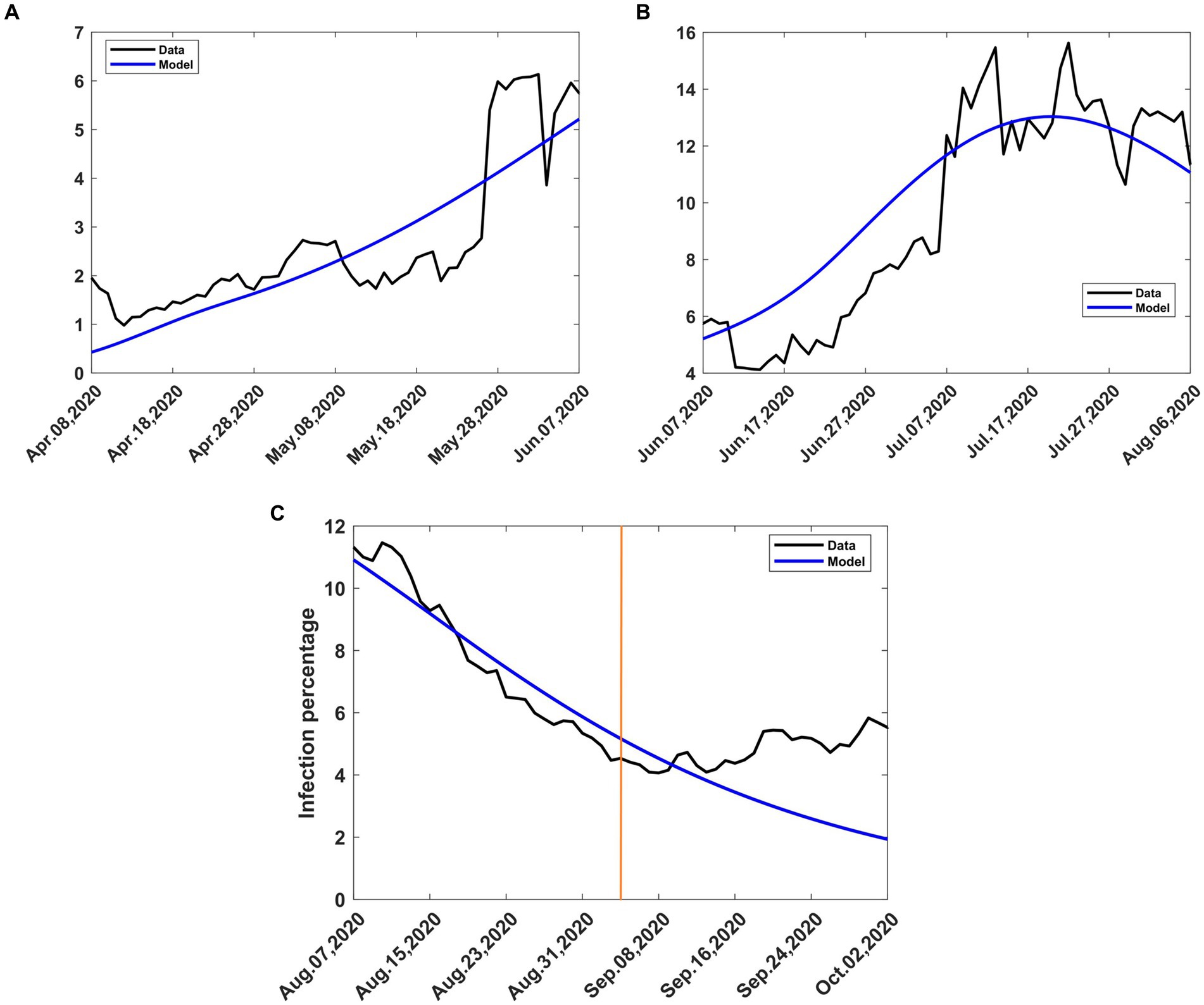
Figure 6. Observed and computed infection percentages during various periods of intervention. Recovery rate, γ = 0.053811; death rate, δ = 0.015. (A) Mitigation, 9th April to 8th June 2020, incoming transmission rate, β_b = 0.188919 (B) Relaxation, 9th June 2020 to 8th August 2020, incoming transmission rate, β_b = 0.10692 (C) Extended relaxation, 9 August 2020 to 3rd September 2020, transmission rate, β_t = 0.14113. The orange vertical line intersects the data at the start of the second wave.

3.2.2 Relaxation from 9th June 2020 to 8th August 2020

As a result of the adverse effects of mitigation, the government relaxed some of the mitigation measures from 9th June 2020 to 8th August 2020. To study the effect of different relaxation strategies, we developed scenarios by varying the fraction c in the transmission rate in Equations (8, 9). We took into account the fact that the Kenyan government had received advice from modellers to take action on relaxation measures considering scenarios involving an increase in transmission by 20, 40, and 60% from the mitigation period (27). To extend the scope of scenarios, we added three more percentages and thus considered the consequence of increasing the transmission by 0% (c = 0, no change), 10% (c = −0.1), 20% (c = −0.2), 40% (c = −0.4), 60% (c = −0.6) and 80% (c = −0.8). The negative values of c are by the explanations given in Section 2.3.1. We chose the incoming transmission rate for relaxation as the mitigation value, namely β_b = 0.10692 as given in Section 3.2.1. Using this value and m = 15 in Equations (8, 9), we solved system (4) from 9th April 2020 to stability. Figure 7 shows the infection curves associated with different values of c. Each curve shows the trajectory of the infection as a result of a one-time relaxation on 9th June 2020, without subsequent interventions. The infection peaks are seen to increase with the increase in $\left|c\right|.$ There is no significant difference in when the peaks appear, depending on c, as was the case for mitigation.

Figure 7

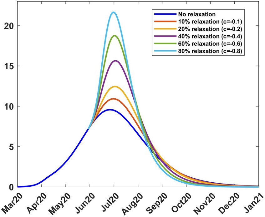
Figure 7. Infection percentages for various relaxation scenarios. Relaxation started on 9th June 2020. Solutions extend to stability. Incoming transmission rate, β_b = 0.10692; recovery rate, γ = 0.053811; death rate, δ = 0.015.

Table 3 shows how varying c affects the transmission rate, reproduction number, and infection. It is noted that as $\left|c\right|$increases, the peak infection and the reproduction number increase. Further increase in $\left|c\right|$leads to a situation where, for c = −0.8 or 80% relaxation, we have ${\mathcal{R}}_0=2.98$ , thus exceeding the basic reproduction number of 2.76. This reflects the fact that the rapid lifting of mitigation measures can result in an outbreak of faster spreading COVID-19, as has been reported in several countries since the outbreak of the disease. Public health advice is that mitigation measures should not be relaxed too rapidly. Table 3 also gives the infection at the end of the relaxation period, namely, 9th August 2020. The model thus enables the planner to forecast, on 9th June 2020, the level of infection when relaxation ends.

Table 3

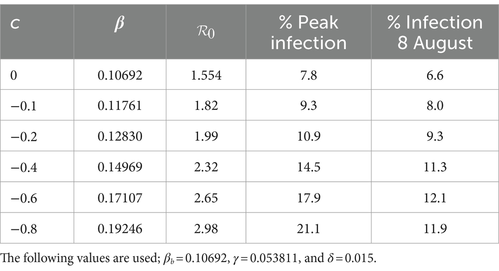
Table 3. Scenarios involving changes in the fraction c under relaxation.

To validate the model, we applied the methods in Section 2.3.4 to the relaxation data and obtained a relaxation fraction of c = −0.32. The result shows that the lifting of the mitigation measures introduced by the government led to an increase in the transmission rate by 32%, over that during the mitigation period, so that the optimum transmission rate during relaxation becomes β_t = 0.14113. The achieved percentage increase is almost halfway between the lowest scenarios, namely 20 and 40%, that the government had been advised to choose (27). The use of c = −0.32, m = 15 and β = 0.10692 in Equations (8, 9) and subsequent solution of system (4) produced results that are compared to the data in Figure 6B. There was still some scatter in the data, and the quality of agreement of the model with the data was still affected.

3.2.3 Extended relaxation from 9th august 2020 to 30th September 2020

The relaxation measures introduced on 9th June 2020 were intended to last for 2 months. However, no major changes in intervention were introduced after 8th August 2020. In Section 2.3.1, we assumed that an intervention remains in effect until another intervention takes place. We consequently treated the period after 8th August 2020 as an extension of the relaxation period in Section 3.2.2. Therefore, the dynamics of the disease was governed by the optimum transmission rate during relaxation, namely, β_t = 0.14113. The use of this value to solve Equations (4a-d) during this period yielded model results that are compared with the data in Figure 6C. There was little scatter of the data, and the model agreed quite well with the data, except towards the end. The divergence at the end was due to the second wave of COVID-19 that emerged in early September 2020. From that moment on, the dynamics of the disease was largely driven by the new variants of interest.

3.2.4 Consolidated results

The actual trajectory followed by the disease is obtained by combining various graphs (Figures 3A, 6A–C) to yield Figure 8 where the modelled 7-day moving averages of percent infection are compared with data. The agreement between the model and data is good, although there was noise in the data at some stages, particularly towards the beginning, when there was still a lot of uncertainty about the collection and processing of information about the new pandemic.

Figure 8

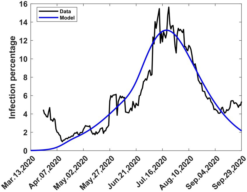
Figure 8. The 7-day moving average of observed and computed percent infections combining mitigation and relaxation strategies during the first wave. Consolidation of graphs (Figures 3A, 6A–C).

In Figure 9 we show graphs of the infection trajectories for the following three scenarios.

Figure 9

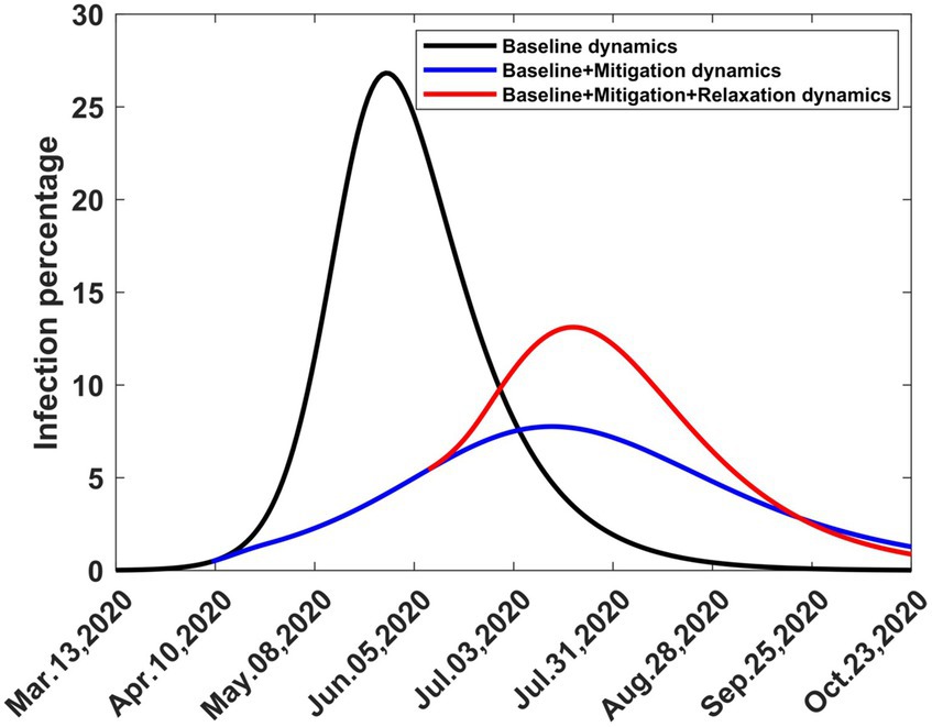
Figure 9. Computed infection percentages depicting three scenarios involving one-time baseline, mitigation, and relaxation strategies. Solutions extend to stability. The baseline started on 13th March 2020, mitigation started on 9th April 2020 and relaxation started on 9th August 2020.

3.2.4.1 Scenario 1 (Baseline dynamics)

What would have happened if COVID-19 had erupted in Kenya on 13th March 2020 and had been allowed to spread without any intervention?

3.2.4.2 Scenario 2 (Baseline + mitigation dynamics)

What would have happened if COVID-19 had erupted in Kenya on 13th March 2020 and had spread without any intervention, but was followed by one-time mitigation on 9th April 9, 2020?

3.2.4.3 Scenario 3 (Baseline + mitigation + relaxation dynamics)

What would have happened if COVID-19 had erupted in Kenya on 13th March 2020 and had spread without any intervention, but was followed by one-time mitigation on 9th April 2020 and one-time relaxation on 9th June 2020?

These graphs show how the infection peak is reduced due to mitigation and then raised due to relaxation, but not to the same level it could have reached if the disease had been allowed to spread without intervention. The third scenario occurred, as shown in Figure 8, but was interrupted by the emergence of the second wave in September 2020.

4 Conclusion

In this study, we developed a mathematical model for intervention that takes into account mitigation, which leads to a decrease in the disease transmission rate, and relaxation, which leads to an increase in the transmission rate. Previous researchers had developed models that could only handle mitigation. We computed the dynamics of COVID-19, using the SIRD model and baseline data of COVID-19 in Kenya and obtained parameter values that yielded a reproduction number, ${\mathcal{R}}_0=2.76$ . This result agrees well with solutions by other methods (31). We focused on the case where the death rate was known so that we needed to estimate the transmission and recovery rate only. However, this method can be extended to estimate the death rate. Our model produces an infection curve that closely follows the observed trends. The model depends on the mitigation and relaxation fractions, which can be assigned to various scenarios while investigating the effects of intervention on disease infection. From the observed infection values, we validated the model by computing the mitigation and relaxation fractions. We determined that the mitigation measures enacted on 9th April 2020 resulted in a reduction of 43.7% of the disease burden from the baseline while there was an increase of 32% due to the relaxation measures enacted on 9th June 2020.

As currently formulated, the model does not detect sub-waves and spikes within the period of intervention. This is partly due to a constant intervention ratio. We propose to vary this ratio, according to fluctuations in the wave, to enable us to detect the sub-waves and spikes. It is also necessary to investigate how the model can be modified to allow accurate prediction of disease trends as data collection proceeds. Another area of investigation is how the model can be extended to detect the formation of the 2nd and subsequent waves and to simulate their development.

Data availability statement

Publicly available datasets were analyzed in this study. This data can be found at: https://www.health.go.ke/covid-19.

Author contributions

WO: Writing – review & editing, Writing – original draft, Validation, Methodology, Investigation, Formal analysis, Conceptualization. VJ: Writing – review & editing, Writing – original draft, Visualization, Validation, Software, Methodology, Formal analysis, Data curation. WB: Writing – review & editing, Writing – original draft, Investigation, Funding acquisition, Data curation.

Funding

The author(s) declare financial support was received for the research, authorship, and/or publication of this article. Publication cost provided by the Department of Research and Development, the Kenya Medical Research Institute (KEMRI), P.O. Box 54840–00200, Nairobi, Kenya.

Acknowledgments

The authors acknowledge Alice Wangui Wachira, Anne Kinyua, and Lucy Nyanchama for their assistance with data collection.

Conflict of interest

The authors declare that the research was conducted in the absence of any commercial or financial relationships that could be construed as a potential conflict of interest.

Publisher’s note

All claims expressed in this article are solely those of the authors and do not necessarily represent those of their affiliated organizations, or those of the publisher, the editors and the reviewers. Any product that may be evaluated in this article, or claim that may be made by its manufacturer, is not guaranteed or endorsed by the publisher.

Supplementary material

The Supplementary material for this article can be found online at: https://www.frontiersin.org/articles/10.3389/fams.2024.1365184/full#supplementary-material

References

1. Worldometer. Available at: https://www.worldometers.info/coronavirus/country/kenya/ Accessed on diverse dates from March 2020 to 30th November 2023).

Google Scholar

2. Coronaviridae study Group of the International Committee on taxonomy of viruses. The species severe acute respiratory syndrome-related coronavirus: classifying 2019-nCOV and naming it SARS-CoV-2. Nat Microbiology. (2020) 5:536–44. doi: 10.1038/s41564-020-0695-z

PubMed Abstract | Crossref Full Text | Google Scholar

3. Wan, Y, Shang, J, Graham, R, Baric, RS, and Li, F. Receptor recognition by the novel coronavirus from Wuhan: an analysis based on decade-long structural studies of sars coronavirus. J Virol. (2020) 94, 1–9. doi: 10.1128/JVI.00127-20

PubMed Abstract | Crossref Full Text | Google Scholar

4. World Health Organization (2020). Modes of transmission of virus causing COVID-19: Implications for IPC precaution recommendations: Scientific brief, 27 march 2020. Technical report, WHO/2019-nCoV/Sci_Brief/Transmission_modes/2020.2.

Google Scholar

5. World Health Organization. Report of the WHO-China Joint Mission on Coronavirus Disease 2019 (COVID-19), 16–24 February 2020.

Google Scholar

6. Biggerstaff, M, Cauchemez, S, Reed, C, Gambhir, M, and Finelli, L. Estimates of the reproduction number for seasonal, pandemic, and zoonotic influenza: a systematic review of literature. BMC Infec Dis. (2014) 14:480. doi: 10.1186/1471-2334-14-480

PubMed Abstract | Crossref Full Text | Google Scholar

7. ASM. Available at: https://asm.org/Articles/2020/July/COVID-19-and-the-Flu (Accessed February 11, 2021).

Google Scholar

8. CDC. Available at: https://www.cdc.gov/flu/symptoms/flu-vs-covid19.htm (Accessed February 11, 2021).

Google Scholar

9. Thornley, S, and Morris, AJ. Rapid response to “the COVID-19 elimination debate needs correct data”. BMJ. (2020) 371:2020. doi: 10.1136/bmj.m3883

Crossref Full Text | Google Scholar

10. Ciao, L., and Liu, Q.. COVID-19 modeling:a review. Available at: https://www.medrxiv.org/content/10.1101/2022.08.22.22279022v2, (2022).

Google Scholar

11. Cintra, PHP, Citeli, MF, and Fontinele, FN. Mathematical models for describing and predicting the COVID-19 pandemic crisis. (2020). doi: 10.48550/arXiv.2006.02507

Crossref Full Text | Google Scholar

12. Anastassopoulou, C, Russo, L, Tsakris, A, and Siettos, C. Data-based analysis, modelling and forecasting of the COVID-19 outbreak. PLoS One. (2020) 15:e0230405. doi: 10.1371/journal.pone.0230405

PubMed Abstract | Crossref Full Text | Google Scholar

13. Caccavo, D . Chinese and Italian COVID-19 outbreaks can be correctly described by a modified SIRD model. medRxiv. (2020). https://www.medrxiv.org/content/10.1101/2020.03.19.20039388v3.full

Google Scholar

14. Iboi, EA, Sharomi, OO, Ngonghala, CN, and Gumel, AB. Mathematical modeling and analysis of COVID-19 pandemic in Nigeria. Math Biosci Eng. (2020) 17:7192–220. doi: 10.3934/mbe.2020369

PubMed Abstract | Crossref Full Text | Google Scholar

15. Malinzi, J, Juma, VO, Madubueze, CE, Mwaonanji, J, Nkem, GN, Mwakilama, E, et al. COVID-19 transmission dynamics and the impact of vaccination: modelling, analysis and simulations. R Soc Open Sci. (2023) 10:221656. doi: 10.1098/rsos.221656

Crossref Full Text | Google Scholar

16. Serhani, M, and Labbardi, H. Mathematical modelling of COVID-19 spreading with asymptotic infected and interacting people. J Appl Math Comput. (2020). doi: 10.1007/512190-02-01421-9

Crossref Full Text | Google Scholar

17. Ignacio, B, Arguedas, HF, Camacho, A, and Saldanã, F. Modeling the transmission dynamics and the impact of the control interventions for the COVID-19 epidemic outbreak. Math Biosci Eng. (2020) 17:4165–83. doi: 10.3934/mbe.2020231

Crossref Full Text | Google Scholar

18. Eikenberry, SE, Mancuso, M, Iboi, E, Phan, T, Eikenberry, K, Kuang, Y, et al. To mask or not to mask: modeling the potential for face mask use by the general public to curtail the COVID-19 pandemic. Infect Dis Model. (2020) 5:293–308. doi: 10.1016/j.idm.2020.04.001

Crossref Full Text | Google Scholar

19. van Wees, J-D, Osinga, S, van der Kuip, M, Tanck, M, Hanegraf, M, Dluymaekers, M, et al. Forecasting hospitalization and ICU rates of the COVID-19 outbreak: an efficient SEIR model. Bull World Health Organ. (2020)

Google Scholar

20. Elsheikh, SMAS, Abbas, MK, Bakheet, MA, and Degoot, AM. A mathematical model for the transmission of coronavirus disease (COVID-19) in Sudan. ResearchGate. (2020). doi: 10.13140/RG.2.2.24167.27043/1

Crossref Full Text | Google Scholar

21. Naraigh, LO, and Byrne, A. Piecewise-constant optimal control strategies for controlling the outbreak of COVID-19 in the Irish population. Math Biosci. (2020) 330:108496. doi: 10.1016/j.mbs.2020.108496

PubMed Abstract | Crossref Full Text | Google Scholar

22. Piccolomini, EL, and Zama, F. Monitoring Italian COVID-19 spread by an adaptive SEIRD model. PLoS One. 15:e0237417. doi: 10.1371/journal.pone.0237417

Crossref Full Text | Google Scholar

23. Ogana, W, Juma, VO, and Bulimo, WD. A SIRD model applied to COVID-19 dynamics and intervention strategies during the first wave in Kenya. medRxiv. (2021) Available at: https://www.medrxiv.org/content/10.1101/2021.03.17.21253626v1

Google Scholar

24. First Case of Coronavirus Disease Confirmed in Kenya. Available at: https://www.health.go.ke/first-case-of-coronavirus-disease-confirmed-in-kenya/ (Accessed December 18th, 2020).

Google Scholar

25. Ministry of Health, Kenya. Available at: https://www.health.go.ke/ (Accessed on diverse dates from March 2020 to 8th November 2021).

Google Scholar

26. Kenya Gazette Supplement No. 41. The public health act (cap.242). The public health (COVID-19 restriction of movement of persons and related measures) rules. 16th April (2020), pp.655–659.

Google Scholar

27. Presidential Addresses on COVID-19. (2021). Available at: https://www.president.go.ke (Accessed on diverse dates from March 2020 to February 2021).

Google Scholar

28. Chowell, G, Viboud, C, Simonsen, L, Miller, M, and Alonso, WJ. The reproduction number of seasonal influenza epidemics in Brazil, 1996–2006. Proc R Soc B Biol Sci. (2010) 277:1857–66.

Google Scholar

29. Chong, K, Goggins, W, Zee, B, and Wang, M. Identifying meteorological drivers for the seasonal variations of influenza infections in a subtropical city—Hong Kong. Int J Environ Res Public Health. (2015) 12:1560–76. doi: 10.3390/ijerph120201560

PubMed Abstract | Crossref Full Text | Google Scholar

30. Juma, V.O. Modelling influenza incidence in relation to meteorological parameters in Kenya (MSc dissertation, University of Nairobi). (2015).

Google Scholar

31. Frost, I, Craig, J, Osena, G, Hauck, S, Kalanxhi, E, Schueller, E, et al. Modeling COVID-19 transmission in Africa: country-wise projections of total and severe infections under different lockdown scenarios. BMJ Open. (2021) 11:e044149. doi: 10.1136/bmjopen-2020-044149

PubMed Abstract | Crossref Full Text | Google Scholar

32. Lopez, Cesar . MATLAB optimization techniques. Apress, (2014).

Google Scholar