Numerical methods for solving second-order initial value problems of ordinary differential equations with Euler and Runge-Kutta fourth-order methods

This paper presents two standard numerical methods for solving second order initial value problems for ordinary differential equations (ODEs). The Euler and the Runge-Kutta fourth-order methods are applied without any discretization or restrictive assumptions for solving ODEs. The numerical solutions obtained by the two methods are in good agreement with the exact solutions. The convergence and error analysis which are discussed demonstrate the effectiveness of the methods. The results obtained from the two numerical methods show that the RK4 method is appropriate, consistent, convergent, quite stable, and more accurate than the Euler's method.

1 Introduction

Ordinary differential equations (ODEs) are mathematical equations that describe the relationship between a function and its derivatives. They are widely used in various fields of science, engineering and mathematics to model physical, biological, and dynamical systems [1–5]. Solving ODEs analytically can often be challenging or even impossible for complex differential equations [6–8]. Therefore, numerical methods play a crucial role in approximating solutions to these equations. The initial value problem (IVP) is a specific type of ODE problem where the values of the unknown function and its derivative(s) are specified at a given initial point. Many researchers developed different methods for solving ordinary differential equations (ODEs) with the initial value problem. Many authors have attempted to solve initial value problems (IVPs) to obtain high accuracy rapidly by using different methods such as the spactral method, the, the Euler's method and Runge Kutta fourth (RK4) order method and some other methods.

Jhnson and Lee explored the application of spectral methods to solve second-order IVP ODEs [9]. The authors employed Legendre polynomials as basis functions and developed spectral schemes to approximate the solution with high accuracy and rapid convergence rates. The advantages of spectral methods in terms of solution accuracy and numerical examples to validate their approach are discussed. Spectral methods are based on representing the solution as a series of basis functions, such as Legendre polynomials, Fourier series or Chebyshev polynomials [6, 10, 11]. By discretizing the problem on a set of collocation points, the unknown function can be approximated by a truncated Legendre polynomial series. These methods provide exponential convergence and are particularly effective for smooth or periodic solutions. It is worth noting that spectral methods, such as the Fourier or Chebyshev methods, have their own advantages for solving ODEs. They are typically more accurate, rapid convergence rates and efficient for problems with only smooth and periodic solutions. Euler's method is straightforward to implement and understand, making it a popular choice for beginners in numerical analysis [5, 11]. It involves only simple arithmetic operations. Euler's method requires fewer computations compared to more complex methods, such as RK4. Hence, it can be computationally more efficient for simple and low-dimensional problems. Since Euler's method only uses information from the previous step to approximate the next step, it can provide a quick estimate of the solution, especially when speed is prioritized over accuracy. RK4 is a higher-order method, which means it provides more accurate approximations compared to Euler's method for a given step size [6, 11, 12]. It achieves this by using multiple evaluations of the derivative at different points within the step, resulting in a smaller truncation error. RK4 is a versatile method that can handle various types of problem, including those with stiff equations and irregular behavior [9]. It is widely used and considered to be one of the most accurate and reliable numerical methods for solving ODEs. Compared to Euler's method, RK4 exhibits better stability properties, making it more suitable for problems that require higher accuracy over longer integration intervals [6, 12]. While there are more advanced and sophisticated numerical methods available, Euler's method and the Runge-Kutta fourth-order method strike a balance between simplicity, efficiency, accuracy, and stability when solving second-order IVPs of ODEs. Euler's method is a basic, easy-to-implement method, while the Runge-Kutta fourth-order method provides higher accuracy, numerical stability, and better control over the solution's accuracy. The choice between these methods depends on the specific problem characteristics, accuracy requirements, available computational resources, and desired trade-offs between accuracy and computational efficiency. Euler's method and Runge-Kutta methods provide a practical and reliable alternative for general second order IVPs of ODEs but spectral methods are accurate and efficient for problems with smooth and periodic solutions. Although extensive research has been conducted on numerical methods for solving first-order IVPs of ODEs, there is a noticeable gap in the literature regarding specialized methods for solving second-order IVPs. Second-order IVPs are more complex due to their involving second derivatives, and applying first-order methods may result in inaccurate solutions or numerical instability. The lack of comprehensive studies on numerical methods tailored for second-order IVPs highlights the need to bridge this gap in the literature. It is crucial to develop and evaluate specialized numerical methods that can reliably and efficiently solve second-order IVPs of ODEs. The aim of this study is to investigate and compare the performance of two widely used numerical methods, namely the Euler method and the Runge-Kutta fourth-order method, in approximating solutions to second-order IVP of ODEs. The study of numerical methods for solving second-order IVP of ODEs with Euler's method and the Runge-Kutta fourth-order method holds significant importance in the field of numerical analysis and scientific computing. Understanding the strengths and limitations of these methods can help researchers, engineers, and scientists select the most appropriate approach for solving ODEs based on specific requirements such as accuracy, efficiency and stability. This knowledge can also aid in optimizing computational algorithms to solve ODEs and providing reliable solutions for real-world problems. In this paper we apply Eulers and fourth order Runge-Kutta method for solving initial value problem of second order ordinary differential equation. A more robust and intricate numerical technique is the Runge-Kutta fourth-order methods. The Runge-Kutta fourth-order (RK4) method generally exhibits better convergence properties compared to Euler's method when solving second-order initial value problems (IVPs) of ordinary differential equations (ODEs). We take an example of a second-order ordinary differential equation to verify our proposed formulation.

2 Problem formulation

In this section, we consider two numerical methods to find approximate solutions of the initial value problem (IVP) of the second-order ordinary differential equation having the following form [9].

$\begin{array}{ll}{y}^{\prime \prime }=f(x,y(x),y^{\prime }(x)),y(d)=\alpha ,y^{\prime }(d)=\beta ,d\le x\le e& (1)\end{array}$

Where $y^{\prime \prime }=\frac{d^{2}y}{d{x}^2}$ , $y^{\prime }=\frac{dy}{dx}$ and f(x, y(x), y′(x)) is the given function and y(x) is the solution of Equation (1). To solve the second-order IVP of ODE by using the Euler and Runge-Kutta fourth-order methods, the second-order initial value problems of ODE can be transformed into a system of first-order initial value problems, which allows the use of standard numerical methods that are widely employed. This approach is commonly known as the first-order system approach and it is indeed not new. In the context of the current study focusing on Euler's method and the Runge-Kutta fourth order (RK4) method, the novelty lies in the analysis and comparison of these specific numerical methods for solving the first-order system derived from the original second-order initial value problem. Although the idea of transforming a second-order initial value problem into a system of first-order problems is not innovative, the analysis and comparison of specific numerical methods applied to the derived first-order system can provide new insights and understanding of their effectiveness, accuracy, stability, convergence properties, and computational efficiency.

We can transform Equation (1) into a system of two first-order ODEs that are grouped as

$\begin{array}{ll}\frac{dy}{dx}=z=f(x,y,z),& (2)\end{array}$

$\begin{array}{l}\frac{dz}{dx}=z^{\prime }=f(x,y,z)y(d)=\alpha ,y^{\prime }(d)=\beta ,d\le x\le e.\end{array}$

Thus, instead of solving Equation (1), we can solve Equation (2)

We note that, with y′ = f(x, y, z) = z, Equation (2) represents the second-order initial value problem.

$\begin{array}{l}{y}^{\prime \prime }=f(x,y,y^{\prime }):y(x_0)=y_0,y^{\prime }(x_0)=z_0\end{array}$

2.1 Euler method

The Euler method is a simple numerical technique for solving ordinary second-order differential equations. It approximates the solution by taking small steps along the curve defined by the differential equation. It is a basic explicit method for the numerical integration of an ordinary differential equations. Euler proposed his method for initial value problems (IVP) in 1768 [5, 9, 11]. It is the first numerical method to solve IVP and serves to illustrate the concepts involved in advanced methods. It is important to study this because error analysis is easier to understand.

Now let's consider a general second-order ODE with initial value problem (IVP):

$\begin{array}{ll}{y}^{\prime \prime }=f(x,y(x),y^{\prime }(x)),y(d)=\alpha ,y^{\prime }(d)=\beta & (3)\end{array}$

To apply Euler's method, we first transform Equation (3) in to a system of two first order ODEs. Transform Equation (3) to systems of two first order ODE, let y′ = z and z′ = f(x, y, z), then Equation (3) becomes

$\begin{array}{l}{y}^{\prime }=z=f(x,y,z)\end{array}$

$\begin{array}{l}{z}^{\prime }=f(x,y,z)\end{array}$

With initial condition, y(d) = α, y′(d) = β and z(x) = y′(x).

Now, we can apply the Euler method to this system of first-order ODEs. The Euler method updates the functions y and z at each step as follows:

$\begin{array}{l}{y}_{n+1}=y_n+h{z}_{n}forn=0,1,2,\dots ,\end{array}$

$\begin{array}{l}{z}_{n+1}=z_n+hf(x_n,y_n,z_n)\end{array}$

This is the general formula to solve the second-order ODE with IVP using the Euler method.

2.2 Runge-Kutta fourth order method

This method was devised by two German mathematicians, Runge about 1894 and was extended by Kutta a few years later [6, 11–13]. The Runge-Kutta method is the most popular because it is quite accurate, stable, and easy to programme. This method is distinguished by its order in the sense that it agrees with Taylor's series solution up to terms of h^r where r is the order of the method. It does not require a prior computational analysis of higher derivatives of y ( x) as in Taylor's series method. The Runge-Kutta fourth-order method (RK4) is widely used for solving second-order initial value problems (IVP) for an ordinary differential equation (ODE). Now let's consider a general second-order ODE with initial value problem (IVP):

$\begin{array}{ll}{y}^{\prime \prime }=f(x,y(x),y^{\prime }(x)),y(d)=\alpha ,y^{\prime }(d)=\beta & (4)\end{array}$

To apply the Runge-Kutta method, we first transform Equation (4) into a system of two first-order ODEs. Transform equation (4) to systems of two first order ODE, let y′ = z and z′ = f(x, y, z), then Equation (4) becomes

$\begin{array}{l}{y}^{\prime }=z=f(x,y,z)\end{array}$

$\begin{array}{l}{z}^{\prime }=f(x,y,z)\end{array}$

With initial condition, y(d) = α, y′(d) = β and z(x) = y′(x).

Now, we can apply the Runge-Kutta fourth-order method to this system of first-order ODEs. The Runge-Kutta fourth order method updates the functions y and z at each step as follows:

The general formula for the Runge-Kutta approximation to solve systems of equations is given by

$\begin{array}{l}{y}_{n+1}=y_n+\frac{1}{6}(k_1+2k_2+{2k}_3+k_4)\end{array}$

$\begin{array}{l}{z}_{n+1}=z_n+\frac{1}{6}(l_1+2l_2+{2l}_3+l_4)\end{array}$

Where k₁ = hf(x_n, y_n, z_n)

$\begin{array}{l}{l}_1=hf(x_n,y_n,z_n)\\ k_2=hf(x_n+\frac{1}{2}h,y_n+\frac{1}{2}{k}_1,z_n+\frac{1}{2}{l}_1)\\ l_2=hf(x_n+\frac{1}{2}h,y_n+\frac{1}{2}{k}_1,z_n+\frac{1}{2}{l}_1)\\ k_3=hf(x_n+\frac{1}{2}h,y_n+\frac{1}{2}{k}_2,z_n+\frac{1}{2}{l}_2)\\ l_3=hf(x_n+\frac{1}{2}h,y_n+\frac{1}{2}{k}_1,z_n+\frac{1}{2}{l}_2)\\ k_4=hf(x_n+h,y_n+k_3,z_n+l_3)\\ l_4=hf(x_n+h,y_n+k_3,z_n+l_3)\\ forn=0,1,2,3,\dots \end{array}$

3 Error analysis

Error analysis is an essential component when studying numerical methods for solving second-order Initial Value Problems (IVPs) of Ordinary Differential Equations (ODEs) using Euler's method and the Runge-Kutta fourth-order (RK4) method [9]. Error analysis allows us to quantify the accuracy of these methods and understand their convergence properties. In numerical methods, the truncation error and the global error are commonly evaluated. The truncation error in Euler's method arises from the linear approximation of the derivative [14, 15]. It is proportional to the step size h, used in the numerical scheme. Specifically, the truncation error is of order O(h)², meaning that by halving the step size, the error typically decreases by a factor of four. The truncation error in RK4 arises from the approximation of the derivative at various internal points within the step. It is proportional to the step size h, increased to the power of five. Therefore, the truncation error of RK4 is of order O(h)⁵, which is significantly smaller than Euler's method [16]. The global error in Euler's method is the cumulative effect of the truncation error at each step throughout the integration interval [17]. As the number of steps increases, the global error accumulates, resulting in a larger discrepancy between the numerical solution and the exact solution. The global error in RK4 is significantly smaller compared to Euler's method [15]. Due to its higher order of accuracy, the cumulative effect of the truncation error is reduced, resulting in a more accurate approximation of the exact solution. It is important to note that while RK4 has a smaller truncation error and is typically more accurate than Euler's method, the step size h, also plays a role. The accuracy of the solution will depend on how small we make the step size h [18]. If |y(x_n)-y_n| = 0, then a numerical technique is considered as convergent. Where the exact solution is denoted by y_n and the approximate solution by y(x_n).

Using a smaller step size can improve the accuracy of both methods; however, it can also increase computational cost [19]. In error analysis, it is common to compare the numerical solutions obtained using Euler's method and RK4 to an analytically available exact solution or a solution obtained using a more accurate method (such as a higher-order Runge-Kutta method). By comparing the errors, we can assess the convergence properties of the methods and determine their suitability for a specific problem. In order to verify the accuracy of the suggested methods, we examine first-order initial value problem ODE in this study. MATLAB software is used to obtain the approximate solution for the two numerical methods that are proposed, at different step sizes. The formula for calculating the maximum error is defined by $e_r={max}_{0\le x\le steps}(|y(x_n)-y_n|)$.

3.1 Numerical example

This section examines a numerical example to verify which numerical techniques converge to an analytical solution more quickly. Errors and numerical solutions are calculated.

Example 1: We consider the initial value problem y^′′−3y′+2y = 0 , y(0) = −1 , y′(0) = 0 on the interval 0 ≤ x ≤ 1 with h = 0.1. Then the exact solution to the given problem is given by y(x) = e^2x− 2e^x.

The approximate results and maximum errors are obtained and shown in Tables 1–4 and the graphs of the numerical solutions are shown as follows in Figures 1–6 from (a)-(r).

Table 1

Table 1. Comparison between Runge–Kutta fourth order and Euler method with exact solution for step size h = 0.1.

Table 2

Table 2. Comparison between Runge–Kutta-fourth order and Euler's method with exact solution for step size h = 0.05.

Table 3

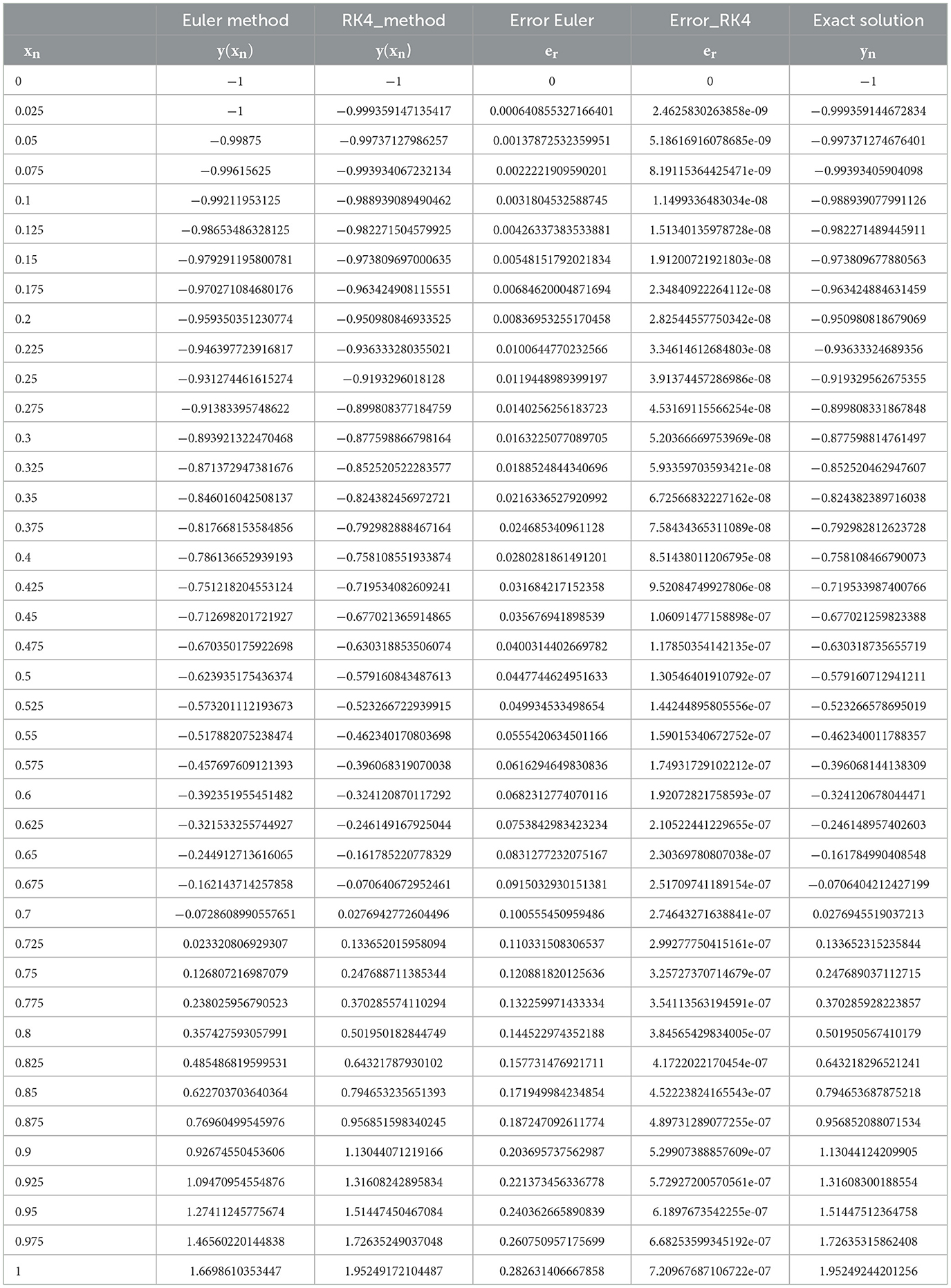
Table 3. Comparison between Runge–Kutta-fourth order and Eulers method with exact solution for step size h = 0.025.

Table 4

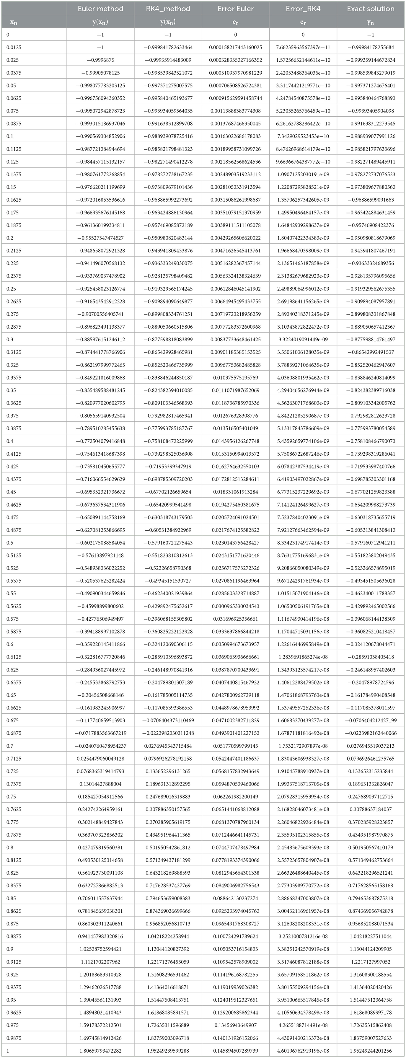
Table 4. Comparison between Runge–Kutta fourth order and Euler's method with exact solution for step size h = 0.0125.

Figure 1

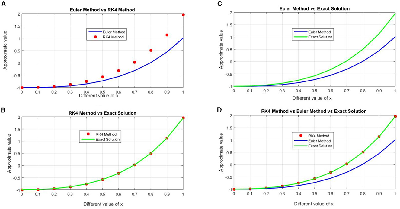
Figure 1. Exact and approximate numerical Solutions for h = 0.1, (A) graph of the approximate solution for Eulers and Runge-Kutta fourth order, (B) graph of the approximate solution of Exact and Runge-Kutta fourth order, (C) graph of the approximate solution for Eulers and Exact, and (D) graph of approximate solutions for Euler, Runge-Kutta forth order methods and exact solution.

Figure 2

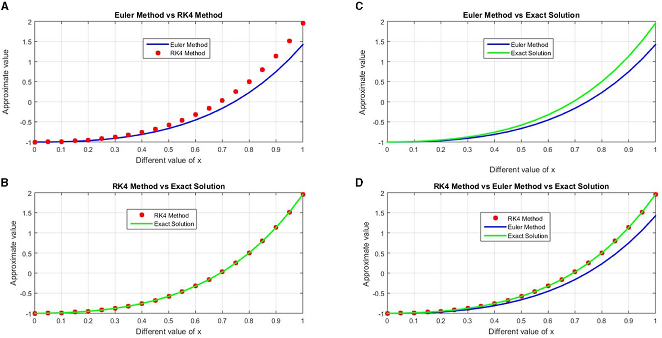
Figure 2. Exact and approximate numerical solutions for h = 0.05, (A) graph of the approximate solution for Eulers and Runge-Kutta fourth order, (B) graph of the approximate solution of Exact and Runge-Kutta fourth order, (C) graph of the approximate solution for Eulers and Exact, and (D) graph of approximate solutions for Euler, Runge-Kutta forth order methods and exact solution.

Figure 3

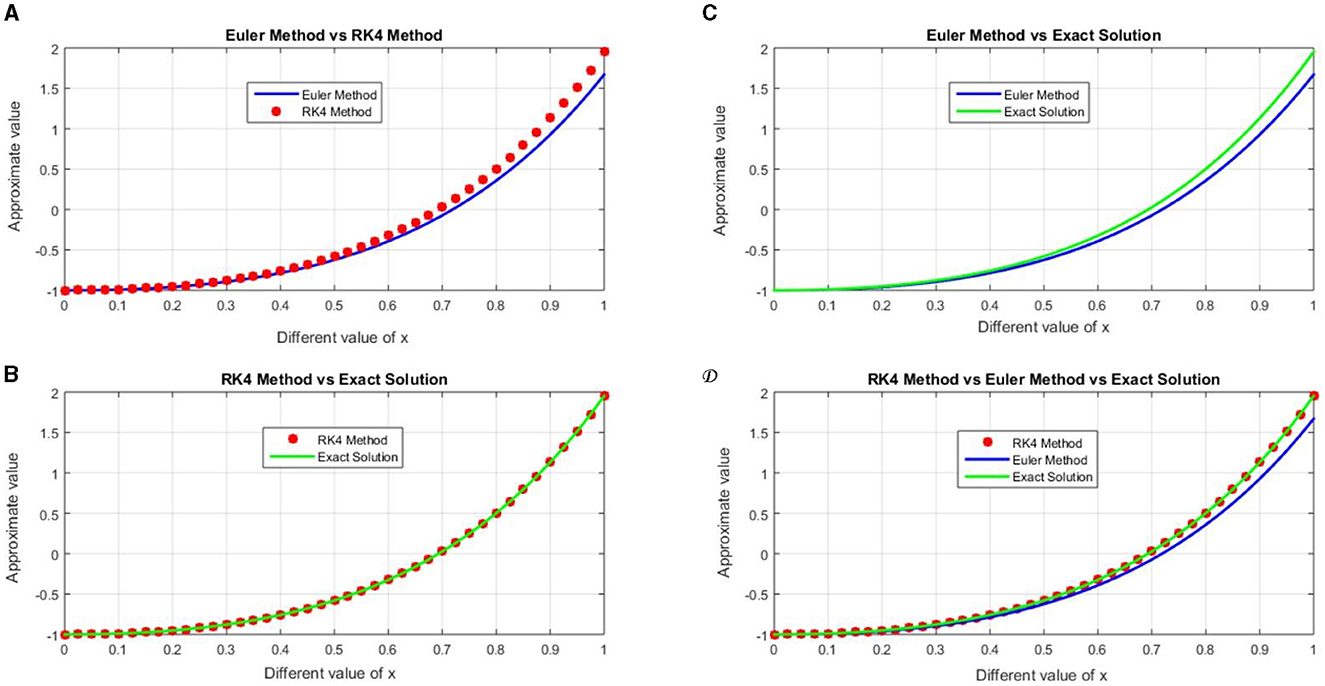
Figure 3. Exact and approximate numerical solutions for h = 0.025, (A) graph of the approximate solution for Euler's and Runge-Kutta fourth order, (B) graph of the approximate solution of Exact and Runge-Kutta fourth order, (C) graph of the approximate solution for Euler's and Exact, and (D) graph of approximate solutions for Euler, Runge-Kutta forth order methods and exact solution.

4 Discussion of results

In this work the obtained results are shown in the Tables 1–4 and graphically representations are show in the Figures 1–7. The Tables 1–4 shows that the comparison of the two desired methods Euler's and Runge-Kutta fourth order method with the exact solution and also the Figures 1–4 shows that the graph of the approximate solution for Euler and Runge-Kutta methods for each step size h. The approximated numerical solution is calculated with the step size h = 0.1, 0.05, 0.025, 0.125. The approximate solution of Euler's and Runge-Kutta fourth order methods have different values for the same step size h for each iteration for example when we compared the accuracy of the Euler and Runge-Kutta fourth order method with sizes h = 0.1 and h = 0.05, then approximated solution with the step size h = 0.1 has less accurate then the approximated solution with the step size h = 0.05 because the error of approximate values for h = 0.1 is greater than the error for h = 0.05 in each iterations. This shows that the Euler's method with h = 0.1 and h = 0.05 does not converges to the exact solution. Similarly for the step sizes h = 0.025 and h = 0.0125, then approximate solution with the step size h = 0.025 has less accurate than the approximate the solution with the step size h = 0.0125 because of the approximate solution with the step size h = 0.0125 has less absolute error then the approximated solution for h = 0.025. This shows that the Euler's method with h = 0.1 and h = 0.05 does not converges to the exact solution but for h = 0.025 and h = 0.0125 Converges slowly to exact solution. The Runge-Kutta fourth order method with the same step size also the approximate solution obtained for h = 0.1 and h = 0.05 converges gradually to exact solution but the approximate for h = 0.025 and h = 0.0125 converges fatly to exact solution. This shows that as the step size decreases the accuracy the approximate solution also increases. The Figures 5, 6 shows that the approximate solution of Euler and Runge-Kutta fourth order method with the same step size respectively. According to Figure 5 the graph of the approximate solution for Runge-Kutta fourth order method are approximately all are overlapped because of little difference between approximate solutions of Runge-Kutta methods with Exact solution (i.e., error) for each h values. From the Figure 6 also the graph of approximated solutions for Euler's method has the gap between two consecutives step sizes this shows that Euler's method has maximum absolute error compared to Runge-Kutta fourth order for same step size. Graph of approximated solutions for h = 0.0125 is above the graph of approximated value for h = 0.1, 0.05, 0.025 this means that the graph of approximated solution approach's to the graph of exact solution as step size decreases but the graph for approximated solution for h = 0.1 is under the graph of approximated solution for h = 0.05, 0.025, 0.0125 this means that it away from the graph of exact solution and it has maximum error for h = 0.1. In the Figure 7 the graph of maximum absolute error for Euler and Runge-Kutta fourth order for each step size are plotted. The graph of error for Euler's method in Figure 7 for h = 0.1 is above h = 0.05, 0.025, and 0.0125 this shows the approximate solution for h=0.1 has maximum error then all approximated solution for h = 0.05, 0.025, 0.0125 but for h = 0.0125 the error graph is below h = 0.05, 0.025, and 0.1 this shows that the absolute error for h = 0.0125 is less then all other approximated solution for h = 0.05, 0.025, and 0.1 for every iteration. Additionally, error analysis for Runge-Kutta method in Figure 7 the graph of error for each step size resembles overlapped to x-axis that means the error for Runge-Kutta is almost tends to zero. From the Figure 7 we observed that Runge-Kutta fourth order converges fastly then the Euler's method with the same step size. The absolute error for each step size h of Euler and Runge-Kutta fourth order methods tends to zero as the step size tends to zero. Although the fourth order Runge-Kutta method is more accurate than the Euler's approach, which only requires one-fourth the step size, it is arduous and takes four evaluations per step size. Finally, we noticed that, as the tables and figures show, the fourth order Runge-Kutta method is the most effective approach for solving second order initial value problem for ordinary differential equations, and that it is converging more quickly than the Euler method.

Figure 4

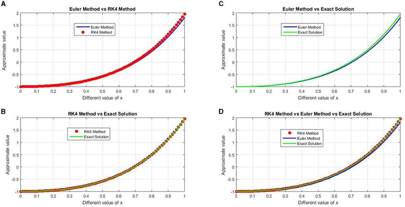
Figure 4. Exact and approximate numerical Solutions for h = 0.0125, (A) graph of the approximate solution for Euler's and Runge-Kutta fourth order, (B) graph of the approximate solution of Exact and Runge-Kutta fourth order, (C) graph of the approximate solution for Eulers and Exact, and (D) graph of approximate solutions for Euler, Runge-Kutta forth order methods and exact solution.

Figure 5

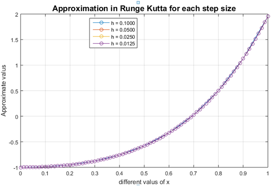
Figure 5. Approximate value for Runge-Kutta fourth order method for each step size.

Figure 6

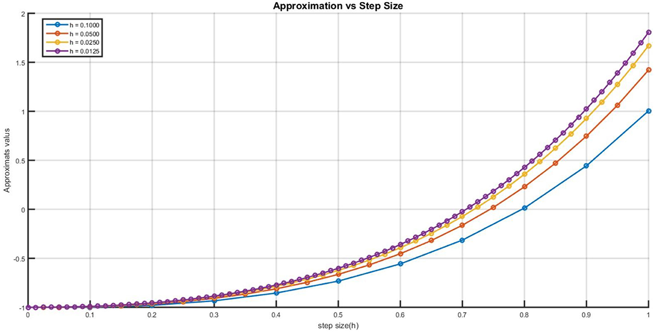
Figure 6. Approximate value for each step size in Euler method.

Figure 7

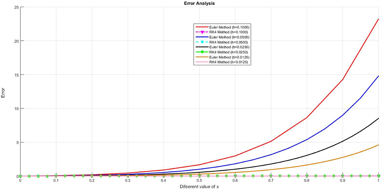
Figure 7. The approximated error for Euler and Runge-Kutta fourth order for different step size.

5 Conclusion

In this work, we have discussed Euler's and fourth order Runge-Kutta method for solving second order initial value problems that provides efficient solutions. To achieve the desired accuracy of the numerical solution it is necessary to take step size small. From the tables and figures, we can see that accuracy of the method obtained for decreasing the step size h. The numerical solutions obtained by the two methods are in good agreement with the exact solutions. However, by comparing the results of the two methods, we state that the RK4 Method is appropriate, consistent, convergent, quite stable, and more accurate than the Euler's method and it is widely used in numerical solutions of second order initial value problems in ordinary differential equations. Our research will be helpful in many scientific areas where numerical computations are needed.

Data availability statement

The original contributions presented in the study are included in the article/supplementary material, further inquiries can be directed to the corresponding author.

Author contributions

YW: Conceptualization, Data curation, Investigation, Methodology, Resources, Software, Supervision, Validation, Visualization, Writing—original draft, Writing—review & editing, Formal analysis, Project administration. HM: Conceptualization, Data curation, Investigation, Methodology, Resources, Software, Supervision, Validation, Visualization, Writing—original draft, Writing—review & editing. BB: Conceptualization, Data curation, Formal analysis, Investigation, Methodology, Project administration, Resources, Software, Supervision, Validation, Visualization, Writing—original draft, Writing—review & editing.

Funding

The author(s) declare that no financial support was received for the research, authorship, and/or publication of this article.

Conflict of interest

The authors declare that the research was conducted in the absence of any commercial or financial relationships that could be construed as a potential conflict of interest.

Publisher's note

All claims expressed in this article are solely those of the authors and do not necessarily represent those of their affiliated organizations, or those of the publisher, the editors and the reviewers. Any product that may be evaluated in this article, or claim that may be made by its manufacturer, is not guaranteed or endorsed by the publisher.

References

1. Sobczyk K. Stochastic Differential Equations: With Applications to Physics and Engineering. Cham: Springer Science & Business Media (2001).

Google Scholar

2. Zhu SP. An exact and explicit solution for the valuation of American put options. Quantitative Financ. (2006) 6:229–42. doi: 10.1080/14697680600699811

Crossref Full Text | Google Scholar

3. Hamming R. Numerical Methods for Scientists and Engineers. Chelmsford, MA: Courier Corporation (2012).

Google Scholar

4. Chapra SC. Numerical Methods for Engineers. New York, NY: Mcgraw-Hill. (2010).

Google Scholar

5. Brissaud A, Frisch U. Solving linear stochastic differential equations. J Mathematic Phys. (1974) 15:524–34. doi: 10.1063/1.1666678

Crossref Full Text | Google Scholar

6. Denis B. An Overview of Numerical and Analytical Methods for solving Ordinary Differential Equations. Cornell University (2020). Available online at: http://arxiv.org/abs/2012.07558

Google Scholar

7. Butcher JC. The Numerical Analysis of Ordinary Differential Equations: Runge-Kutta and General Linear Methods. London: Wiley-Interscience (1987).

Google Scholar

8. Jator SN, Li J. Boundary value methods via a multistep method with variable coefficients for second order initial and boundary value problems. Int J Pure Appl Mathematics. (2009) 50:403–20.

Google Scholar

9. Hossain MJ, Alam MS, Hossain MB. A study on numerical solutions of second order initial value problems (IVP) for ordinary differential equations with fourth order and Butcher's fifth order Runge-Kutta methods. Am J Comput Appl Mathematics. (2017) 7:129–37. doi: 10.5923/j.ajcam.20170705.02

Crossref Full Text | Google Scholar

10. Hussain K, Ismail F, Senu N. Solving directly special fourth-order ordinary differential equations using Runge–Kutta type method. J Comput Appl Math. (2016) 306:179–99. doi: 10.1016/j.cam.2016.04.002

Crossref Full Text | Google Scholar

11. Kamruzzaman M, Nath MC. A comparative study on numerical solution of initial value problem by using Euler's method, modified Euler's method and Runge–Kutta method. J Comput Mathematic Sci. (2018) 9:493–500. doi: 10.29055/jcms/784

Crossref Full Text | Google Scholar

12. Cromer A. Stable solutions using the Euler approximation. Am J Phys. (1981) 49:455–9. doi: 10.1119/1.12478

Crossref Full Text | Google Scholar

13. Hossen M, Ahmed Z, Kabir R, Hossan Z. A comparative investigation on numerical solution of initial value problem by using modified Euler method and Runge-Kutta method. IOSR-JM. (2019) 12:2278–5728. doi: 10.9790/5728-1504034045

Crossref Full Text | Google Scholar

14. Hindmarsh AC, Petzold LR. Algorithms and software for ordinary differential equations and differential-algebraic equations, Part I: Euler methods and error estimation. Computers in Physics. (1995) 9:34–41. doi: 10.1063/1.168536

Crossref Full Text | Google Scholar

15. Okeke AA, Tumba P, Anorue OF, Dauda A. Analysis and comparative study of numerical solutions of initial value problems (IVP) in ordinary differential equations (ODE) with Euler and Runge-Kutta methods. AJER. (2019) 8:6–15.

Google Scholar

16. Amir Taher K. Comparison of Numerical Methods for Solving a System of Ordinary Differential Equations: Accuracy, Stability and Efficiency. Lowa City, IA: Johan Wiley, and Sons (2009). p. 81.

Google Scholar

17. Neto AR, Rao KR. A stochastic approach to global error estimation in ODE multistep numerical integration. J Comput Appl Math. (1990) 30:257–81. doi: 10.1016/0377-0427(90)90279-9

Crossref Full Text | Google Scholar

18. Gustafsson K, Söderlind G. Control strategies for the iterative solution of nonlinear equations in ODE solvers. SIAM J Sci Comp. (1997) 18:23–40. doi: 10.1137/S1064827595287109

Crossref Full Text | Google Scholar

19. Atkinson K, Han W, Stewart DE. Numerical Solution of Ordinary Differential Equations. New York, NY: John Wiley & Sons (2009).

Google Scholar