This study proposes and analyzes a deterministic mathematical model to describe the dynamics of corruption transmission. We began by proving that the solution to the model is bounded and positive. The next-generation matrix approach is used to compute the basic reproduction number (${\mathcal{R}}_0$) in relation to corruption-free equilibrium. The Jacobian and Lyapunov functions are used to show that corruption-free equilibrium is asymptotically stable in both locally and globally when ${\mathcal{R}}_0<1$, and otherwise, an endemic corruption equilibrium develops. Furthermore, the sensitivity of the model's parameters was investigated. The findings demonstrate that religious precepts govern public education. The two sectors most susceptible to corruption control are education and corrections. The study recommends investing more in the provision of public education to citizens by creating awareness among all and including it in the education curriculum and religious leaders to teach their followers seriously about the impact of corruption as well as the use of jail as punishment. The numerical simulation results agreed with the analytical results.

1 Introduction

The World Bank [1] defines corruption as an illicit activity committed for personal gain and benefit by public (government) or private (business) officials who abuse their position of authority or influence. According to Abdulrahman [2], individuals may be corrupted and then gradually grow into the most corrupt individuals. It is indistinct in terms of color, shape, odor, collusion, secrecy, stealth, and shamelessness [3]. According to Rothstein [4], corruption has a negative impact on a nation's ability to flourish and is widespread and present to varied degrees throughout the world. It is a cancer to the development of the economy, the social order, and the political system [5].

Several mathematical studies have been conducted to better understand the causes and methods for preventing corruption around the world [6]. For example, Danford et al. [7] quantitative modeling and analysis of Tanzanian corruption dynamics using control measures demonstrated a direct relationship between the study's parameters and the basic reproduction number (${\mathcal{R}}_0$). According to their research, the corruption-free equilibrium is globally asymptotically stable for ${\mathcal{R}}_0<1$. An endemic equilibrium persists and the corruption-free equilibrium point is unstable if ${\mathcal{R}}_0>1$. While it is challenging to totally remove corruption, it might be lessened by raising wages in the public sector and decreasing poverty.

In their study, Akanni et al. [8] examined a deterministic mathematical model that considers the impact of society on morally upright people to explain the transmission dynamics of corruption. The model's positivity and boundedness are established, and the next-generation matrix approach is used to get the basic reproduction number. The research demonstrates that when ${\mathcal{R}}_0<1$, corruption-free equilibrium is asymptotically stable both locally and globally. Additionally, whenever ${\mathcal{R}}_0>1$, the endemic equilibrium point is asymptotically stable both locally and globally. Globally, a great deal of research has been conducted on how pandemics evolve. The evaluation and forecasting of the corruption pandemic's spread, together with the identification of its parameters, were thoroughly and meticulously examined in the studies [9–15]. A mathematical model of corruption dynamics including stability analysis was created by Nathan and Jackob [13]. In their research, they covered the necessity of sustained engagement and active participation on the side of anti-corruption players such as governments, the commercial sector, academia, civil society, and media.

Over the course of a year, a number of authors have used mathematical models to assess the effects of corruption on national development and the best control strategies for the dynamics of corruption. These authors include [16–24]. In particular, Lemecha [25] constructed and examined a mathematical model with a constant recruitment rate from the total population to investigate the dynamical nature of corruption governing the model. The awareness raised by anti-corruption efforts and in prison counseling was factored into the mathematical model of corruption that was constructed. The analysis shows that the corruption-free equilibrium is locally asymptotically stable whenever the reproduction number is smaller than one. The analytical results were validated using numerical simulation.

As mentioned above, all studies developed mathematical models of corrupt transmission dynamics by viewing different aspects. But many of them did not consider honest individuals become susceptible in one model. But, the honest peoples have a chance to be susceptible due to desire or poverty and also analysis the effects of education, religious, and punishment on transmission dynamics of corruption.

The remainder of this research is as follows: Section 2 presents the mathematical model framework for the propagation of corruption. In Section 3, we investigate the positivity and boundedness of solutions, as well as the stability of the endemic and corruption-free equilibria. Section 4 covers the subject of numerical simulation. Section 5 offers a conclusion at the end.

2 Model formulation

The model formulation and its description were covered in this section. The entire population is split into four classes in this model: susceptible class S(t), which is composed of those who do not participate in any corrupt activity; corrupted class C(t), which is composed of those who actually participate in corrupt behavior; recovered class R(t), those who are stopped from doing any corrupt activity; and those who do not commit corruption are honest class H(t). The entire population is provided by N(t) = S(t) + C(t) + R(t) + H(t).

We assume that the recruitment rate of π increased the susceptible class. The ω rate at which the honest people become vulnerable is caused by poverty or desire. However, susceptible people begin to practice corruption after coming into touch with corrupt people, are persuaded by them at a rate of β, and are moved to the corrupted class; the remaining portion will join the honest class as a result of public education γ and religious instruction η. Corrupted individuals stop doing corruption and join recovery class due to public education, religious, jail at rate ξ, and natural death rate of μ, respectively. Since, the recovery class there is a temporally stay meaning that after short interval of time, individuals leave the class at the rate of (1 − τ)α join susceptible class or the remaining join the honest class at rate of ατ. The flow chart in Figure 1 and the Table 1 depicts the explanation mentioned previously.

Figure 1

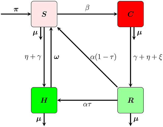
Figure 1. Flow chart of the model.

Table 1

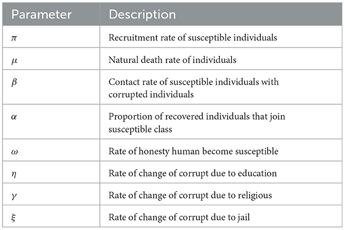
Table 1. Description of parameters.

Putting all model equations together, we obtain the following non-linear system of differential equations:

$\begin{array}{ll}\{\begin{array}{l}\frac{dS}{dt}=\pi -\beta SC+\alpha (1-\tau )R+\omega H-(\gamma +\eta +\mu )S,\\ \frac{dC}{dt}=\beta SC-(\gamma +\eta +\xi +\mu )C,\\ \frac{dR}{dt}=(\gamma +\eta +\xi )C-(\alpha +\mu )R,\\ \frac{dH}{dt}=(\gamma +\eta )S+\alpha \tau R-(\mu +\omega )H,\end{array}& (1)\end{array}$

with initial conditions, S(0) > 0, C(0) ≥ 0, R(0) ≥ 0, and H(0) ≥ 0.

The parameters appearing in the system 1 are described and interpreted in the Table 1.

3 Model analysis

3.1 Non-negativity and invariant region

The constraint on the model's solution is found using the invariant area.

Theorem 1. For the system 1, a positively invariant set is the closed area

$\begin{array}{l}\Omega =\left\{(S,C,R,H)\in R_{+}^4:N(t)\le \frac{\pi }{\mu }\right\}.\end{array}$

Proof 1 Differentiating the entire population N(t) with respect to time t and subtracting all values of state variables from system 1, we obtain

$\begin{array}{ll}\frac{dN}{dt}=\pi -\mu N,& (2)\end{array}$

and then solving the Equation 2, we obtain

$\begin{array}{ll}N(t)=\frac{\pi }{\mu }+\left[N_0-\frac{\pi }{\mu }\right]e^{-\mu t}.& (3)\end{array}$

Hence, from Equation (3) $N(t)\to \frac{\pi }{\mu }$ as t → ∞ that indicates N(t) ≤ $\frac{\pi }{\mu }$. Therefore, Ω is the feasible region of system 1.

Theorem 2. The solution set (S(t), C(t), R(t), H(t)) of system 1 is positive for all t ≥ 0 for non-negative initial conditions.

Proof 2 Let us take the first equation from the system 1. Without loss of generality, omit all terms from the equation that do not contain the state variable S because our intention is to test for positivity of only S(t).

$\begin{array}{ll}\frac{dS}{dt}\ge -(\beta C+\gamma +\eta +\mu )S.& (4)\end{array}$

Integrating Equation (4) with respect to time and applying separable method of variables with the initial condition, we get

$\begin{array}{ll}S(t)\ge S(0)e^{-\int (\beta C+\gamma +\eta +\mu )dt}>0.& (5)\end{array}$

Hence, Equation (5) shows that S(t) > 0. Similarly, for others. This proves that the solution of system 1 is positive for all t ≥ 1.

3.2 Corruption-free equilibrium

When there is no corruption in the community, or C = 0, we have what is known as corruption-free equilibrium (CFE). After finding the non-corrupted state variable by solving for the right hand side of system 1, we obtain

$\begin{array}{l}{\Xi }_0=\left(\frac{\pi }{\mu (\gamma +\eta +\omega +\mu )},0,0,\frac{\pi (\gamma +\eta )}{\mu (\omega +\mu )(\gamma +\eta +\omega +\mu )}\right).\end{array}$

3.3 Basic reproduction number

The average number of secondary cases that could result from the introduction of one corrupt person into a completely susceptible community is known as the basic reproduction number (R₀) [17]. The next-generation matrix technique described in [9, 26] can be used to obtain it. Rewriting the system 1 is the first stage, and it should begin with the recently compromised class.

$\begin{array}{ll}\frac{dC}{dt}=\beta SC-(\gamma +\eta +\xi +\mu )C.& (6)\end{array}$

Then, the basic reproduction number of the model is the spectral radius of the next-generation matrix FV⁻¹, where F is the matrix of new corrupted terms and V is the matrix of transition terms. Then Equation (6) can be written as the form of F-V, where

$\begin{array}{ll}\mathcal{F}=\beta SC\text{ and }\mathcal{V}=(\gamma +\eta +\xi +\mu )C.& (7)\end{array}$

The Jacobian matrices of $\mathcal{F}$ and $\mathcal{V}$ of Equation (7) are obtained by differentiating with respect to C as follows:

$\begin{array}{ll}F=\frac{\partial \mathcal{F}}{\partial C}=\beta S,V=\frac{\partial \mathcal{V}}{\partial C}=\gamma +\eta +\xi +\mu .& (8)\end{array}$

Then, evaluating Equation (8) at the corruption-free equilibrium point, we get

$\begin{array}{ll}F=\frac{\partial \mathcal{F}}{\partial C}=\frac{\pi \beta }{\mu (\gamma +\eta +\omega +\mu )},V=\frac{\partial \mathcal{V}}{\partial C}=\gamma +\eta +\xi +\mu .& (9)\end{array}$

Hence, in Equation (9), the matrix V(Ξ₀) is invertible and thus

$\begin{array}{l}{V}^{-1}=\frac{1}{\gamma +\eta +\xi +\mu }.\end{array}$

By the principle of next-generation matrix,

$\begin{array}{l}{\mathcal{R}}_0=\frac{\pi \beta }{\mu \left[(\gamma +\eta +\omega +\mu )(\gamma +\eta +\xi +\mu )\right]}.\end{array}$

3.4 Local stability of CFE points

Theorem 3. The corruption-free equilibrium point is locally asymptotically stable if ${\mathcal{R}}_0<1$ and unstable otherwise.

Proof 3 To proof this theorem, first linearize the system 1 by using Jacobian matrix method, and then evaluating at the corruption-free equilibrium point, we get

$\begin{array}{ll}J=\left(\begin{array}{cccc}-(\gamma +\eta +\mu )& -\frac{\pi \beta }{\mu (\gamma +\eta +\omega +\mu )}& \alpha (1-\tau )& \omega \\ 0& \frac{\pi \beta }{\mu (\gamma +\eta +\omega +\mu )}-(\gamma +\eta +\xi +\mu )& 0& 0\\ 0& \gamma +\eta +\xi & -(\alpha +\mu )& 0\\ \gamma +\eta & 0& \alpha \tau & -(\mu +\omega )\end{array}\right).& (10)\end{array}$

Expanding the characteristic equation |J − λI| = 0 Equation (10), we get two eigenvalues

$\begin{array}{l}{\lambda }_1=\frac{\pi \beta }{\mu (\gamma +\eta +\omega +\mu )}-(\gamma +\eta +\xi +\mu ),\\ =(\gamma +\eta +\xi +\mu )({\mathcal{R}}_0-1)<0,\end{array}$

only if ${\mathcal{R}}_0<1$ and λ₂ = −(α + μ) < 0. The remaining roots are the solution to the following equation:

$\begin{array}{ll}{\lambda }^2+\lambda C+D=0,& (11)\end{array}$

where C = (γ + η + 2ω + 2μ) and D = μ(γ + η + ω + μ). Thus, Equation (11) has a strictly negative real root if and only if C > 0, D > 0, and CD > 0, according to the Rourth-Hurwitz criterion that we applied. Given that C > 0 is the sum of positive parameters, it is evident that this is the case. As a result, Ξ₀ is locally asymptotically stable.

3.5 Global stability of CFE point

Theorem 4. The corruption-free equilibrium of the system 1 is globally asymptotically stable if ${\mathcal{R}}_0<1$ and unstable if ${\mathcal{R}}_0>1$.

Proof 4 To prove the global stability of the corruption-free equilibrium we use the method of Lyapunov functions. Define

$\begin{array}{ll}L=\frac{1}{2}{C}^2,\text{ then }\frac{dL}{dt}=\frac{\partial L}{\partial C}\frac{dC}{dt}.& (12)\end{array}$

Now, from system 1, we have

$\begin{array}{l}\frac{dC}{dt}=\beta SC-(\gamma +\eta +\delta +\xi +\mu )C.\end{array}$

Therefore, Equation (12) become

$\begin{array}{l}\frac{dL}{dt}=\frac{\partial L}{\partial C}\frac{\partial C}{\partial t},\\ =C(\beta SC-(\gamma +\eta +\xi +\mu ))C,\\ =C^2(\beta S-(\gamma +\eta +\xi +\mu )).& (13)\end{array}$

Since $S^{*}=\frac{\pi }{\mu (\gamma +\eta +\omega +\mu )}$ and then, from Equation (13), we get

$\begin{array}{l}\frac{dL}{dt}=C^2\left(\frac{\pi \beta }{\mu (\gamma +\eta +\omega +\mu )}-(\gamma +\eta +\xi +\mu )\right),\\ =C^2(\gamma +\eta +\xi +\mu )\left(\frac{\pi \beta }{\mu (\gamma +\eta +\omega +\mu )(\gamma +\eta +\xi +\mu )}-1\right),\\ =C^2(\gamma +\eta +\xi +\mu )({\mathcal{R}}_0-1).& (14)\end{array}$

Hence, from Equation (14), we have

$\begin{array}{l}\frac{dL}{dt}\le 0\text{for }{\mathcal{R}}_0<1.\end{array}$

Therefore, every solution to the system 1 with initial conditions in Ω that approaches the corruption-free equilibrium point as time t tends to infinity whenever ${\mathcal{R}}_0<1$ does so in accordance with LaSalle's invariant principle [27].

3.6 Stability analysis of endemic equilibrium

The endemic equilibrium point of the model is denoted by Ξ_* and it occurs when the correction persists in the community. To obtain the endemic equilibrium, we equate all the right hand side of system 1 to zero and solve them. Consequently, to solve for, it is necessary to make the provided Equations 1 equal to zero. This implies:

$\begin{array}{r}\pi -\beta SC+\alpha (1-\tau )R+\omega H-(\gamma +\eta +\mu )S=0,\\ \beta SC-(\gamma +\eta +\xi +\mu )C=0,\\ (\gamma +\eta +\xi )C-(\alpha +\mu )R=0,\\ (\gamma +\eta )S+\alpha \tau R-(\mu +\omega )H=0.& (15)\end{array}$

The persistent recruitment equilibrium, solving for the remaining variables, we get

$\begin{array}{l}(\gamma +\eta +\delta +\xi )C^{*}-(\alpha +\mu )R^{*}=0,\\ (\alpha +\mu )R^{*}=(\gamma +\eta +\delta +\xi ),\\ R^{*}=\frac{(\gamma +\eta +\delta +\xi )}{\alpha +\mu }.\end{array}$

Next, the value of S^* can be found as follows from Equation (15):

$\begin{array}{l}\beta S^{*}{C}^{*}-(\gamma +\eta +\delta +\xi +\mu +{\mu }_c)C^{*}=0,\\ \beta S^{*}=(\gamma +\eta +\delta +\xi +\mu +{\mu }_c),\\ S^{*}=\frac{(\gamma +\eta +\delta +\xi +\mu +{\mu }_c)}{\beta }.\end{array}$

Finally,

$\begin{array}{l}(\gamma +\eta )S^{*}+\alpha \tau R^{*}-(\mu +\omega )H^{*}=0,\\ (\mu +\omega )H^{*}=(\gamma +\eta )S^{*}+\alpha \tau R^{*},\\ (\mu +\omega )H^{*}=\frac{(\gamma +\eta )(\gamma +\eta +\delta +\xi +\mu +{\mu }_c)}{\beta }+\frac{\alpha \tau (\gamma +\eta +\delta +\xi )}{\alpha +\mu },\\ H^{*}=\frac{1}{(\mu +\omega )}\left[\frac{(\gamma +\eta )(\gamma +\eta +\delta +\xi +\mu +{\mu }_c)}{\beta }+\frac{\alpha \tau (\gamma +\eta +\delta +\xi )}{\alpha +\mu }\right].\end{array}$

and

$\begin{array}{l}{C}^{*}=\frac{(\alpha +\mu )\left[(\omega +\mu )({\mathcal{R}}_0-1)+\omega (\gamma +\eta )+\omega (\gamma +\eta )\right]}{\beta \left[\frac{(\omega +\mu )(\alpha +\mu )}{(\gamma +\eta +\xi )}+\frac{\alpha (\omega +\mu )-\alpha \tau }{\gamma +\eta +\xi +\mu }\right]}\end{array}$

Theorem 5. The endemic equilibrium point (EEP) of system 1 at Ξ_* is locally asymptotically stable if ${\mathcal{R}}_0>1$.

Proof 5 We employ the linearizion approach to demonstrate the local stability of the endemic equilibrium point of the system 1. At the endemic equilibrium point, the Jacobian $\mathcal{J}({\Xi }_{*})$ matrix thus becomes

$\begin{array}{ll}\mathcal{J}=\left(\begin{array}{cccc}-(\beta C^{*}+\gamma +\eta +\mu )& -\beta S^{*}& \alpha (1-\tau )& \omega \\ \beta C^{*}& \beta S^{*}-(\gamma +\eta +\delta +\xi +\mu )& 0& 0\\ 0& \gamma +\eta +\delta +\xi & -(\alpha +\mu )& 0\\ \gamma +\eta & 0& \alpha \tau & -(\mu +\omega )\end{array}\right)& (16)\end{array}$

The characteristic equation of the Jacobian matrix 16 at the endemic equilibrium point is also given by:

$\begin{array}{ll}P(\lambda )={\lambda }^4+A_1{\lambda }^3+A_2{\lambda }^2+A_3\lambda +A_4& (17)\end{array}$

where

$\begin{array}{r}{A}_1=(\alpha +\mu )+(\omega +\mu )+(\beta +\gamma +\eta +\delta +\xi +\mu ),\\ A_2=(\beta +\gamma +\eta +\delta +\xi +\mu )(\alpha +\omega +2\mu )+\\ \beta (\gamma +\eta +\delta +\xi +\mu )+\beta \alpha (1-\tau )(\gamma +\eta +\delta +\xi ),\\ A_3=\left[\beta (\gamma +\eta +\delta +\xi +\mu )+\beta \alpha (1-\tau )(\gamma +\eta +\delta +\xi )\right]\\ (\alpha +\omega +2\mu ),\\ A_4=\beta (\gamma +\eta +\delta +\xi +\mu )+\beta \alpha (1-\tau )(\gamma +\eta +\delta +\xi )\\ (\alpha +\mu )(\omega +\mu )\end{array}$

If the characteristic polynomial of Equation (17) satisfies the Routh-Hurwitz requirements, its eigenvalues will be negative. Therefore, if ${\mathcal{R}}_0>1$, the EEP of system 1 will be locally asymptotically stable.

Theorem 6. The endemic equilibrium point (EEP) of system 1 at Ξ_* is glocally asymptotically stable if ${\mathcal{R}}_0>1$.

Proof. To analyze the global stability of the endemic equilibrium point, we construct the Lyapunov function defined by

$\begin{array}{l}L(S^{*},C^{*},R^{*},H^{*})=\frac{1}{2}[(S(t)-S^{*})+(C(t)-C^{*})(R(t)-R^{*})\\ {+(H(t)-H^{*})]}^2& (18)\end{array}$

Computing the derivative of the Equation (18) with respect to time, we obtain as

$\begin{array}{r}\frac{dL}{dt}=\left[(S(t)-S^{*})+(C(t)-C^{*})(R(t)-R^{*})+(H(t)-H^{*})\right]\\ \frac{d}{dt}\left[S+C+R+H\right],\\ =\left[(S(t)-S^{*})+(C(t)-C^{*})(R(t)-R^{*})+(H(t)-H^{*})\right]\\ \frac{dN}{dt}.& (19)\end{array}$

Since

$\begin{array}{llll}\frac{dN}{dt}& \le & \pi -\mu N& (20)\end{array}$

Thus, using Equation (20), Equation (19) becomes

$\begin{array}{l}\frac{dL}{dt}\le [(S(t)-S^{*})+(C(t)-C^{*})(H(t)-H^{*})\\ +(R(t)-R^{*})](\pi -\mu N)\\ \le \left(N-\frac{\pi }{\mu }\right)(\pi -\mu N)& (21)\end{array}$

From Equation (21), we get the following result by rearranging and simplifying the expression

$\begin{array}{l}\frac{dL}{dt}\le \frac{1}{\mu }{(\pi -\mu N)}^2\end{array}$

Therefore,

$\begin{array}{l}\frac{dL}{dt}(S,C,R,H)\le 0and\frac{dL}{dt}=0\\ iffS=S^{*},C=C^{*},R=R^{*},H=H^{*}\end{array}$

Thus, the dominant invariant set in Ω: $\frac{dL}{dt}=0$ is one set C^*. As a result of [27, 28] invariant principle, the corruption endemic equilibrium is globally asymptotically stable in Ω.

3.7 Sensitivity analysis

Sensitivity analysis is used to find model parameters that significantly affect ${\mathcal{R}}_0$. We computed using the definition of the normalized sensitivity index given in [9, 29].

Definition 1. The normalized sensitivity index of a variable, ${\mathcal{R}}_0$, that depends differentiability on a parameter, u, is defined as

$\begin{array}{ll}{\Lambda }_u^{{\mathcal{R}}_0}=\frac{\partial {\mathcal{R}}_0}{\partial u}\times \frac{u}{{\mathcal{R}}_0},& (22)\end{array}$

for u represents all the basic parameters.

The sensitivity analysis for the basic reproduction number of system 1 using Equation (22) of its ${\mathcal{R}}_0$ is given by:

$\begin{array}{l}{\Lambda }_{\beta }^{{\mathcal{R}}_0}=\frac{\partial {\mathcal{R}}_0}{\partial \beta }\times \frac{\beta }{{\mathcal{R}}_0}=1>0,\\ {\Lambda }_{\omega }^{{\mathcal{R}}_0}=\frac{\partial {\mathcal{R}}_0}{\partial \omega }\times \frac{\omega }{{\mathcal{R}}_0}=\frac{\omega (\gamma +\eta )}{(\gamma +\eta +\omega +\mu )(\omega +\mu )}>0,\\ {\Lambda }_{\gamma }^{{\mathcal{R}}_0}=\frac{\partial {\mathcal{R}}_0}{\partial \gamma }\times \frac{\gamma }{{\mathcal{R}}_0}=-\frac{\gamma (2\gamma +2\eta +2\mu +\delta +\xi )}{(\gamma +\eta +\omega +\mu )(\gamma +\eta +\delta +\xi +\mu )}<0,\\ {\Lambda }_{\eta }^{{\mathcal{R}}_0}=\frac{\partial {\mathcal{R}}_0}{\partial \eta }\times \frac{\eta }{{\mathcal{R}}_0}=-\frac{\eta (2\gamma +2\eta +2\mu +\delta +\xi )}{(\gamma +\eta +\omega +\mu )(\gamma +\eta +\delta +\xi +\mu )}<0,\\ {\Lambda }_{\xi }^{{\mathcal{R}}_0}=\frac{\partial {\mathcal{R}}_0}{\partial \xi }\times \frac{\xi }{{\mathcal{R}}_0}=\frac{-\xi }{\gamma +\eta +\delta +\xi +\mu }<0.\end{array}$

The sensitivity indices of the basic reproductive number with respect to main parameters are found in Table 2.

Table 2

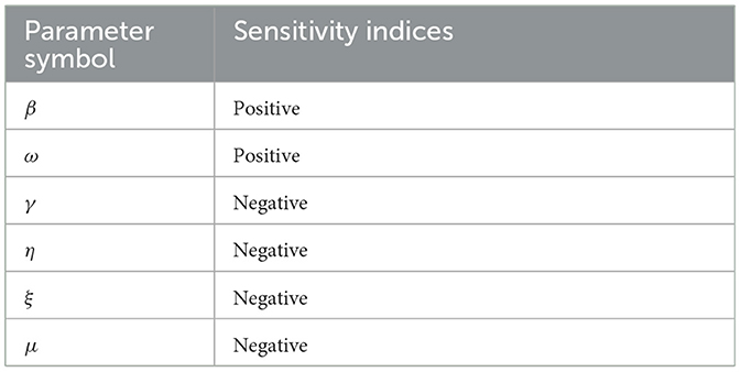
Table 2. Sensitivity indices table.

The equation above contains the fundamental reproductive number's sensitivity indices with regard to the key parameters, and hence, the results demonstrated that while the other parameters stayed constant. If the values of the parameters with positive indices ω and β increase, it indicates that they have a significant influence on the spread of corruption in the community. Additionally, when their values rise, the parameters γ, η, and ξ, whose sensitivity indices are negative, have the effect of lessening the burden of corruption in the community. As a result, stakeholders and policymakers should endeavor to increase the parameters of the negative indices and decrease the good indices. However, increasing human mortality rates to combat corruption epidemics is unethical, so they are not taken into account in the study of sensitivity analysis.

4 Numerical simulations

In this part, we illustrate numerical simulations of the system 1 for different values of the parameters given in the model and illustrate that these simulations are consistent with the qualitative behavior of the system solutions. Our simulations look at how different parameter combinations in the model affect how corruption dynamics are transmitted. We used several parameters with constant variables or with different beginning values in numerical simulation to examine the influence of the parameters on corruption dynamics, thus that S(0) = 210, C(0) = 75, R(0) = 10, and H(0) = 50. The natural death rate is computed as $\mu =\frac{1}{66.71\times 12}$ per month, where 66.71 years is the average life expectancy in Ethiopia [30]. The numerical simulations of the model (1) were conducted by Matlab software using parameters values found in Table 3.

Table 3

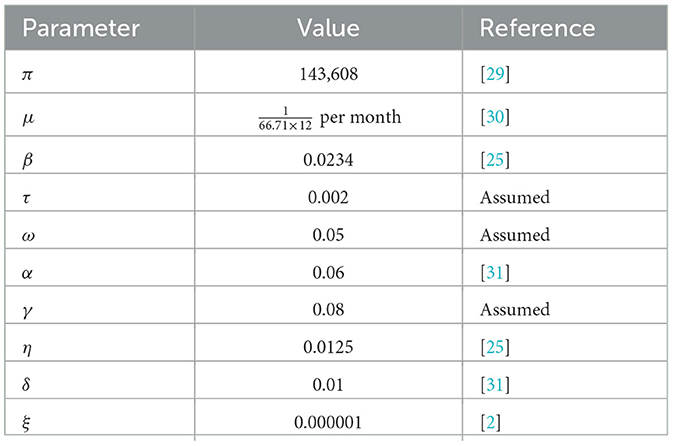
Table 3. Values of parameters used in the simulations.

As demonstrated by Figure 2, the number of corrupt humans rises from t = 0 to t = 3 at the outset because of a rise in the rate of want and poverty in society, which encourage the majority of people to participate in corrupt activities. Due to the fact that some people go to recover from corruption through education, religious instruction, and punishments, the number of corrupt people declines sharply after t = 3. Since some honest persons join susceptible classes at a rate of ω, the number of honest individuals increases from t = 0 to t = 2 due to the natural recovery rate. After that, the number of honest individuals decreases. Because of the presumption that there is temporary immunity at the recovered class, the recovered class stays empty. The number of people who have recovered from corruption has significantly increased over time because some people have recovered as a result of mass education, natural causes, religious beliefs, and incarceration. Figure 2 illustrates how ${\mathcal{R}}_0=2.2906>0$ is the explanation for the rise in the number of corrupt people. The picture also demonstrates how contact with dishonest people reduced the amount of susceptible individuals.

Figure 2

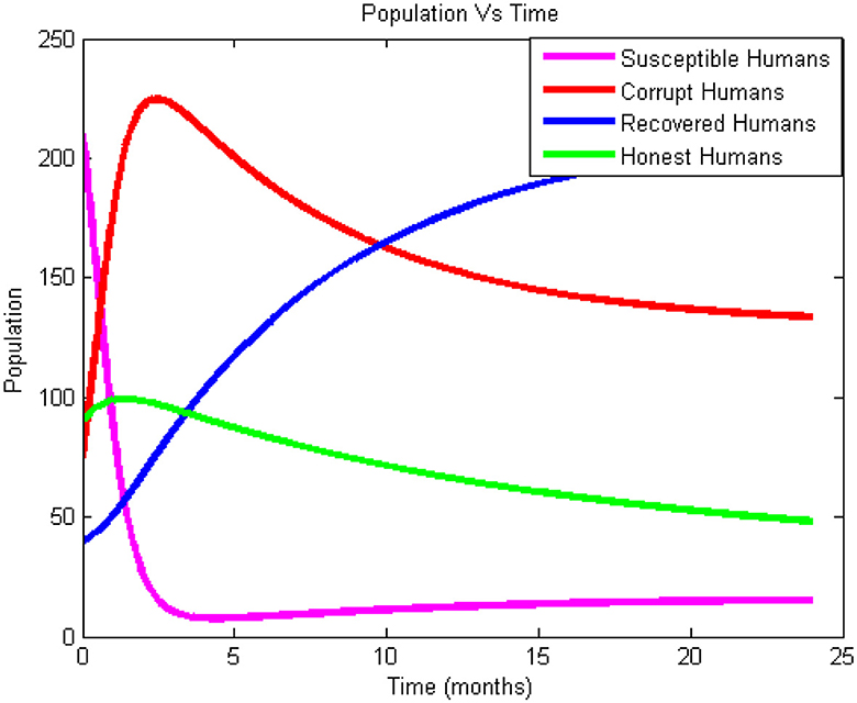
Figure 2. Corruption dynamics of the model.

4.1 Effect of education on the honest and corrupted individuals

Figures 3A, B illustrate how the number of the corrupt individual reduces and the number of the honest individual increases when γ is changed from 0.2 to 0.35. The figure shows us that as we go up, the proportion of corrupt people drops and the proportion of onset people rises. We can see from the simulation results in Figures 3A, B that we can reduce corrupted populations via teaching. Therefore, to raise awareness among the populace, the government should invest more in educating the public about the detrimental effects of corruption. Curriculum developers should also include corruption studies into the curricula at all educational levels.

Figure 3

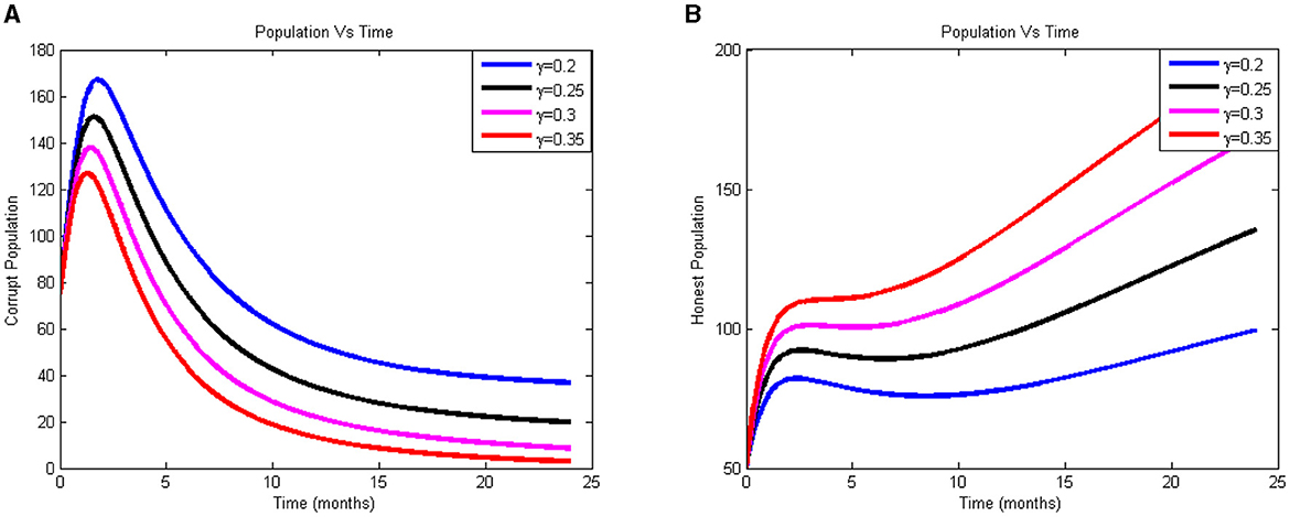
Figure 3. (A) Effect of η on corrupted individuals. (B) Effect of η on honest individuals.

4.2 The effects of religious teaching against corruption

The effect was explored with by varying its value from 0.009 to 0.9, as we can see in Figures 4A, B. The graph indicates that when η rises, the proportion of dishonest people falls and the proportion of truthful people rises. Therefore, the model made the assumption that most adherents had faith in their religious leaders. In this instance, it is imperative that greater religious instruction be incorporated into the national fight against corruption. The model made the assumption that the majority of adherents have faith in their scholars for adding additional religious leaders to the fight against corruption is imperative in this instance in the nation. Corrupt practices have decreased, according to the graph, since t = 2, or about two months after the technique was implemented. The majority of the community can thus benefit from investing in religious instruction, which will lower the rate of corruption in the area.

Figure 4

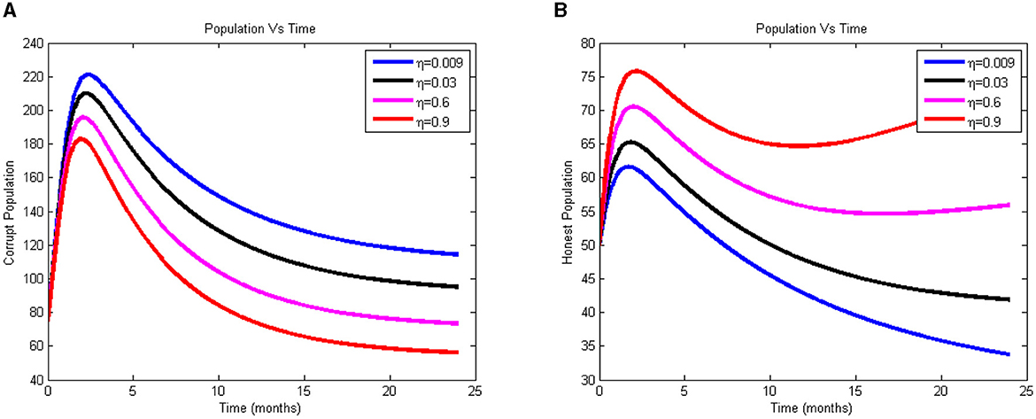
Figure 4. (A) Effect of η on corrupted individuals. (B) Effect of η on honest individuals.

4.3 The effects of prison against corruption

Figure 5 illustrates how, as ξ's value rises, it becomes more significant in reducing the number of corrupted individuals. The chart shows that it raises the number of honest people while decreasing the number of corrupt people. Figure 5 illustrates this point by demonstrating that the more religious leaders educate their followers about corruption as a sin, the fewer corrupt people there are in the community. The model made the assumption that the majority of followers trusted their religious leaders; therefore, more religious leaders need to be involved in the national effort to combat corruption. According to the graph, corruption decreased from t = 3, or roughly three months after the strategy's inception.

Figure 5

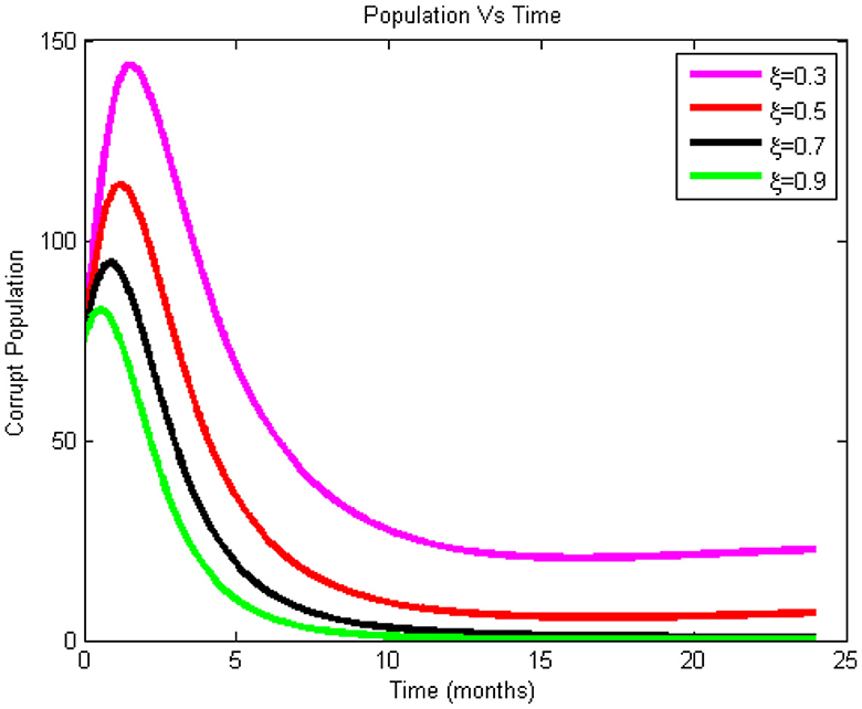
Figure 5. Effect of prison on corrupted individuals.

In general, from stability analysis, sensitivity analysis, and numerical simulation, transmission and recovery rate had a great power in controlling the corruption. Therefore, concerned bodies should try to minimizing transmission rate and maximizing recovered rate to reduce the corruption in the community.

5 Conclusion

This article developed and examined a mathematical model on the dynamics of corruption transmission. First, we demonstrated that the model is both mathematically and epidemiologically well-posed within a certain region. We examined the model using a qualitative study. In addition to calculating the fundamental reproduction number ${\mathcal{R}}_0$, equilibrium point stability was examined. The corruption-free equilibrium point is globally asymptotically stable whenever ${\mathcal{R}}_0$ is smaller than unity, according to Lyapunov's theory. The fundamental reproduction number ${\mathcal{R}}_0$ is directly impacted by the parameters β and α, as can be shown from the analytical study of ${\mathcal{R}}_0$. Since the fundamental reproduction number rises to more than one, the transmission rate from susceptible persons to corrupted individuals is represented by the parameter β. This implies that the higher the contact rate, the more common corruption is in the nation. Therefore, the community's corruption is regulated. The parameters stand for prison, education, and religious instruction, respectively. As these parameters rise, the effective reproduction number falls below one. These results imply that since corruption goes against religious teaching and faith, more work should be done to educate the general people. Additionally, religious leaders should be given more responsibility for effectively educating their followers about the negative impacts of corruption. Therefore, in future deterministic modeling of optimal control strategies for corruption, transmission in two interconnected patches can be developed to analyze the impact of migration.

Data availability statement

The original contributions presented in the study are included in the article/supplementary material, further inquiries can be directed to the corresponding author.

Author contributions

BA: Conceptualization, Data curation, Formal analysis, Funding acquisition, Investigation, Methodology, Project administration, Resources, Software, Supervision, Validation, Visualization, Writing—original draft, Writing—review & editing. HT: Resources, Formal Analysis, Investigation, Validation, Visualization, Writing—review & editing. TK: Supervision, Writing—review & editing. AG: Supervision & Software. DD: Software. AG: Software.

Funding

The author(s) declare that no financial support was received for the research, authorship, and/or publication of this article.

Conflict of interest

The authors declare that the research was conducted in the absence of any commercial or financial relationships that could be construed as a potential conflict of interest.

Publisher's note

All claims expressed in this article are solely those of the authors and do not necessarily represent those of their affiliated organizations, or those of the publisher, the editors and the reviewers. Any product that may be evaluated in this article, or claim that may be made by its manufacturer, is not guaranteed or endorsed by the publisher.

References

1. World Bank. Helping Countries Combat Corruption: The Role of the World Bank. Washington, DC: World Bank (1997).

Google Scholar

2. Abdulrahman S. Stability analysis of the transmission dynamics and control of corruption. Pacific J Sci Technol. (2014) 15:99–113.

Google Scholar

3. Caiden G. “Dealing with administrative corruption”, in Hand-book of Administrative Ethics. Boca Raton: CRC Press. (2001).

Google Scholar

4. Rothstein B. (2011). The Quality of Government: Corruption, Social Trust and Inequality in a Comparative Perspective. Chicago: The University of Chicago Press.

Google Scholar

5. Hathroubi S, Trabelsi H. Epidemic corruption: a bio-economic homology. Eur Scientif J. (2014) 10:46–60.

Google Scholar

6. Li MY. An introduction to Mathematical Modeling of Infectious Diseases (Vol. 2). Cham: Springer. (2018).

PubMed Abstract | Google Scholar

7. Danford O, Kimathi M, Mirau S. Mathematical Modelling and Analysis of Corruption Dynamics with Control Measures in Tanzania. J Math Inform. (2020) 19:57–79. doi: 10.22457/jmi.v19a07179

Crossref Full Text | Google Scholar

8. Akanni J, Akinpelu F, Olaniyi S, Oladipo A, Ogunsola A. Modelling financial crime population dynamics: optimal control and cost-effectiveness analysis. Int J Dynam Cont. (2020) 8:531–44. doi: 10.1007/s40435-019-00572-3

Crossref Full Text | Google Scholar

9. Lazebnik T. Computational applications of extended SIR models: A review focused on airborne pandemics. Ecol Model. (2023) 483:110422. doi: 10.1016/j.ecolmodel.2023.110422

Crossref Full Text | Google Scholar

10. Rose-Ackerman S. The economics of corruption. J Public Econ. (1975) 4:187–203. doi: 10.1016/0047-2727(75)90017-1

Crossref Full Text | Google Scholar

11. Lazebnik T, Bunimovich-Mendrazitsky S, Ashkenazi S, Levner E, Benis A. Early detection and control of the next epidemic wave using health communications: development of an artificial intelligence-based tool and its validation on COVID-19 data from the US. Int J Environ Res Public Health. (2022) 19:16023. doi: 10.3390/ijerph192316023

PubMed Abstract | Crossref Full Text | Google Scholar

12. Mungiu-Pippidi A. “Contextual choices in fighting corruption: lessons learned,” in Hertie School of Goverance: Report commissioned by the Norwegian Agency for Development Cooperation. Berlin: Hertie School of Goverance. (2011).

Google Scholar

13. Nathan OM, Jackob KO. Stability analysis in a mathematical model of corruption in Kenya. Asian Res J Mathemat. (2019) 15:115. doi: 10.9734/arjom/2019/v15i430164

Crossref Full Text | Google Scholar

14. Cuervo-Cazurra A. Corruption in international business. J World Busin. (2016) 51:365382. doi: 10.1016/j.jwb.2015.08.015

Crossref Full Text | Google Scholar

15. Nwajeri UK, Asamoah JKK, Ugochukwu NR, Omame A, Jin Z. A mathematical model of corruption dynamics endowed with fractal-fractional derivative. Results Phys. (2023) 53:106894. doi: 10.1016/j.rinp.2023.106894

Crossref Full Text | Google Scholar

16. Athithan S, Ghosh M, Li XZ. Mathematical modeling and optimal control of corruption dynamics, Asian-Eur J Mathemat. (2018) 11:1850090. doi: 10.1142/S1793557118500900

Crossref Full Text | Google Scholar

17. Keno TD, Legesse FM. Modelling and optimal control strategies of corruption dynamics. Appl Math Inf Sci. (2023) 17:673–683. doi: 10.18576/amis/170416

Crossref Full Text | Google Scholar

18. Waykar SR. Mathematical modelling: a comparatively mathematical study model base between corruption and development. IOSR J Mathemat. (2013) 6:5462. doi: 10.9790/5728-0625462

Crossref Full Text | Google Scholar

19. Wayker SR. Mathematical modelling: a study of corruption in the society of India. Int J Scientif Eng Res. (2013) 4:2303–18.

Google Scholar

20. Lenhart S, Workman JT. Optimal Control Applied to Biological Models. Boca Raton: CRC Press. (2007). doi: 10.1201/9781420011418

Crossref Full Text | Google Scholar

21. Nikolaev PV. Corruption suppression models: the role of inspectors moral level. Computat Mathemat Model. (2014) 25:87102. doi: 10.1007/s10598-013-9210-1

Crossref Full Text | Google Scholar

22. Khan MAU. The corruption prevention model. J Discrete Mathemat Sci Cryptograp. (2000) 3:173–178. doi: 10.1080/09720529.2000.10697905

Crossref Full Text | Google Scholar

23. Gweryina RI, Kura MY, Okwu E. An epidemiological model of corruption with immunity clause in Nigeria. World J Model Simulat. (2019) 15:262–275.

Google Scholar

24. Alemneh HT. Mathematical modeling, analysis, and optimal control of corruption dynamics. Hindawi J Appl Mathemat. (2020) 13:2020. doi: 10.1155/2020/5109841

Crossref Full Text | Google Scholar

25. Lemecha L. Modelling corruption dynamics and its analysis. Ethiop J Sci Sustain Dev. (2018) 5:1327. doi: 10.20372/ejssdastu:v5.i2.2018.34

Crossref Full Text | Google Scholar

26. Van den Driessche P, Watmouch J. Reproduction numbers and sub-threshold endemic equilibria for compartmental models of disease transmission. Math Biosci. (2002) 180:29–48. doi: 10.1016/S0025-5564(02)00108-6

PubMed Abstract | Crossref Full Text | Google Scholar

27. La Salle JP. The Stability of Dynamical Systems. Bangkok: SIAM. (1976).

Google Scholar

28. Temesgen DK, Makinde OD, Obsu LL. Optimal control and cost-effectiveness analysis of SIRS malaria disease model with temperature variability factor. J Mathemat Fundam Sci. (2021) 53:134–163. doi: 10.5614/j.math.fund.sci.2021.53.1.10

Crossref Full Text | Google Scholar

29. Aga BZ, Keno TD, Terfasa DE, Berhe HW. Pneumonia and COVID-19 co-infection modeling with optimal control analysis. Front Appl Math Stat. (2024) 9:1286914. doi: 10.3389/fams.2023.1286914

Crossref Full Text | Google Scholar

30. World Health Organization (WHO);World Health Organization (WHO). Coronavirus Disease 2019. Wuhan: Coronavirus Disease 2019. (2020).

Google Scholar

31. Binuyo AO. Eigenvalue elasticity and sensitivity analyses of the transmission dynamic model of corruption. J Nigerian Soc Phys Sci. (2019) 201:30–4. doi: 10.46481/jnsps.2019.6

Crossref Full Text | Google Scholar