 Dereje Tarekegn Nigatu1*
 Tekle Gemechu Dinka
 Surafel Luleseged Tilahun
- 1Department of Applied Mathematics, Adama Science and Technology University, Adama, Ethiopia
- 2Department of Applied Mathematics, Addis Ababa Science and Technology University, Addis Ababa, Ethiopia
Particle swarm optimization (PSO) algorithm is an optimization technique with remarkable performance for problem solving. The convergence analysis of the method is still in research. This article proposes a mechanism for controlling the velocity by applying a method involving constriction factor in standard swarm optimization algorithm, that is called CSPSO. In addition, the mathematical CSPSO model with the time step attractor is presented to study the convergence condition and the corresponding stability. As a result, constriction standard particle swarm optimization that we consider has a higher potential to balance exploration and exploitation. To avoid the PSO premature convergence, CSPSO modifies all terms of the PSO velocity equation. We test the effectiveness of the CSPSO algorithm based on constriction coefficient with some benchmark functions and compare it with other basic PSO variant algorithms. The theoretical convergence and experimental analyses results are also demonstrated in tables and graphically.
1 Introduction
The optimization techniques are fundamentally important in engineering and scientific computing. The PSO algorithm was first introduced by Kennedy and Eberhart [1] as a stochastic optimization technique of swarm particles (population). The motivation was primarily to model the social behavior of birds flocking. The meta-heuristic optimization algorithms (PSO) work effectively in many areas such as robotics, wireless networks, power systems, job-shop schedules, human healthcare, and classifying or training of ANN (artificial neural network) [2]. In PSO, the potential solutions, called particles, fly through the problem space (domain) by applying their intelligent collective behaviors.
The PSO algorithm is competitive in performance with the well-known huge numbers of variants such as SPSO and CPSO algorithms and is also an efficient optimization framework [3, 4].
Lately, researches on PSO mainly intended on algorithmic implementations, enhancements, and engineering applications with interesting findings derived under the system that assumes a fixed attractor [5]. Nevertheless, a comprehensive mathematical explanation for the general PSO is still quite limited. For instance, the works on stability and convergence analyses are two key problems of great significance that need to be investigated in depth because many of the works have given attention for standard PSO.
The PSO algorithm depends on three parameters (factors): the inertia, cognitive and social weight to guarantee the stability of PSO.
Stability analysis of PSO is mainly motivated by determining which combination of these parameters encourages convergence [6].
The working rule of PSO method is closely tied with the stability analysis, which investigates how the essential factors affect the swarms dynamics, and under what conditions particle swarm converges to some fixed value. For the first time, stability analysis of the particle dynamics was carried out by Clerc and Kennedy [7]. The study indicates that [8] particle trajectories could converge to a stable point. A more generalized stability analysis of the particle dynamics was conducted using the Lyapunov stability theorem [9]. Recently, based on a weak stagnation assumption, Liu [10] studied the order-2 stability of PSO, and a new definition of stability was proposed with an order-2 stable region. Dong and Zhang [11] analyzed order-3 recurrence relation of PSO kinematic equations based on two strategies to obtain the necessary and sufficient conditions of its convergence.
The convergence analysis determines whether a global optimum solution can be achieved when a particle swarm converges. Using stochastic process theory, Jiang et al. [12] presented a stochastic convergence analysis on the standard PSO. Combining with the finite element grid technique, Poli and Langdon [13] set up a discrete model of Markov chain of the bare-bones PSO. An absorbing Markov process model of PSO was developed in Cai et al. [14]. Cai et al. [14] suggested the main factor of convergence analysis is the attaining-state set and proposed an improved method of convergence in terms of the attaining-state set theorem of expansion. The basic PSO is neither a global nor a local search algorithm, based on the convergence criterion of the pure random search algorithm [15, 16]. To yield a lower bound for the time required to optimize any pseudo-Boolean functions with a unique optimum and to justify upper bounds, Dirk et al. [17] assigned an optimum-level argument that is deep-rooted for evolutionary algorithms of particle swarm optimization. The study in Sun et al. [18] discussed the convergence of the quantum-behaved particle swarm optimization (QBPSO) and proved that it is a global convergent algorithm.
As discussed in Per and Carsten [19], stagnation of the convergence properties for basic PSO may be disadvantageous to finding a sufficiently good solution within a logical time, and it may have infinite expected first hitting time on some functions.
Recently, the existing work on the convergence analyses of PSO including documents from 2013 was surveyed by Tarekegn et al. [6]. The stochastic approximation technique on the PSO algorithm was use to prove convergence of swarm in Yuan and Yin [20]. The global convergence of PSO [21] was investigated by introducing the transition probability of particles. Several properties related to the Markov chain were investigated, and it was found that the particle state space is not repeated and PSO is not globally convergent from the viewpoint of the transition probability [22]. Based on the different models of PSO examined [23], the Markov properties of the state sequences of a single particle and swarm one determine the transition probability of a particle. The transition probability of the optimal set is deduced by combining the law of total probability with the Markov properties [24], which proves that SPSO can reach the global optimum in probability. Although many methods in Poli and Langdon [13] have proposed PSO convergence analysis, most analyses are based on the assignment of stochastic systems of the Markov process, which strongly depends on the transition matrix and their eigenvalues. Therefore, when the population size is large, current PSO convergence analyses are very refined and investigate different PSO variants algorithms to obtain a solution that converges to global minimum.
Motivated by our recent study in Tarekegn et al. [6], this article proposes a PSO variant known as CSPSO, an algorithm for optimization problem solving.
A constriction factor integrated with an inertia weight are used for the construction. Fast convergent method to an optimal solution within the search space in a small time of iterations was obtained.
The rest of this study is organized as follows: Section 2 presents related works that include the basic PSO algorithm and its existing variants. In Section 3, the proposed CSPSO algorithm analysis is described in detail, while Section 4 presents comparison results on some variants of PSO such as SPSO and CPSO (implementing with test functions) and provides an in-depth discussion, with a conclusion in Section 5.
2 The PSO algorithm and some related studies
In the PSO with K particles in which each particle is treated as an individual in the D-dimensional space, the position and velocity vectors of the i-th particle at the t-th iteration are
and
, respectively.
In SPSO algorithm [25], at iteration t, the d th dimension of particle i's velocity and position is local best position, is current position, and gt is global best position. Both are updated as
for 1 ≤ i ≤ K; ω is an inertia weight; and c1 and c2 are called acceleration coefficients in real-space, R.
Vector is the best previous position of particle i called personal best (Pbest) position and vector is the position of the best particle among all the particles in the population and called global best (gbest) position. The parameters and are sequences of two different random positive numbers in the uniform random distribution in (0, 1) i.e., U(0, 1).
Generally, the value of is restricted within the interval [−Vmax, Vmax], for each d ∈ {1, 2, …, D}. Without loss of generality, we consider the minimization problem:
Minimize f(X), such that
where f(X) is an objective function continuous almost everywhere and S is a feasible solution space. From (1), the non-homogeneous recurrence relation (NHRR) is obtained as follows: [8]
where .
From NHRR, Pt and gt, for 1 ≤ i ≤ K, are updated, respectively, as follows:
From (2), (3), the process of the particle's velocity and position change can be obtained, respectively, as follows. They are a second-order difference equations
where,
The terms and on the left side of (6), both memorize the past values of position (i.e, the memory item of position). The value of the item on the right side of (6) is obtained from the previous experience of particles (i.e, the learning item of position) and, in particular, is the attractor at the t th iteration in (7).
Now, let
For , and . From (8), means for all t.
Introducing a constriction coefficient in SPSO controls the balance between the cognitive component () and social component () in the velocity equation. The coefficient restricts the particle velocities within a certain range to prevent excessive exploration or exploitation.
2.1 Convergence of some PSO variants
The importance of a hybrid method is to combine different optimization methods to take advantage of the virtues of each of the methods. In addition to standard PSO, several variants of the PSO in Kumar et al. [5] were constructed to improve the performance of PSO.
The SPSO
has a scalar function of position if for a particle, that is particle's update depends only on its previous velocity. This can make the algorithm to stop to flow on the swarm's global best position, even if that position is not a local optimum. For instance, based on (4), the guaranteed convergence PSO, GCPSO, overcomes this problem by using a modified position and velocity update equation for the global best particle, which forces that particle to search for a better position in a confined region around the global best position.
The GCPSO can be used with neighborhood topologies such as star, ring, and Von Neumann. Neighborhoods have a similar effect in the GCPSO [16, 19] as they do in the SPSO. Shi and Eberhart [25] introduced the concept of linearly decreasing inertia weight with generation number into PSO to improve the algorithmic performance.
Particles converge to a weighted average () between their personal and local best positions [8], referred to as a so-called theoretical attractor point (ATP). Kennedy [26] has proposed that the entire velocity update equation is replaced by a random number sampled from a Gaussian distribution (Gd) around the ATP, with a deviation of the magnitude of the distance between the personal and global best. The resultant algorithm is called the bare bones PSO (BBPSO). Kennedy also proposed an alternative bare bones PSO (aBBPSO) [26], where the particle sampled from the previous Gd is reunited with the particle's personal best position. The performance of PSO with a small and a larger nearby region might be better on multimodal and unimodal problems, respectively [27]. Changing dynamically the neighborhood structures has been proposed to avoid insufficiencies in fixed nearby regions [28].
The quantum-behaved particle swarm optimization was proposed to show many advantages to the traditional PSO. Fang et al. [24] proposed a quantum-behaved particle swarm optimization (QBPSO) algorithm and discuss the convergence of QBPSO within the framework of random algorithm's global convergence theorem. Inspired by natural speciation, some researchers have introduced evolution methods into PSO [29, 30]. The problem of premature convergence was studied on a perturbed particle swarm algorithm presented based on the new particle updating strategy [31]. To solve optimization problems, Tang et al. [32] developed a feedback-learning PSO algorithm with quadratic inertia weight, ω. Hybridized PSO with a local search technique for locating optimal solutions for multiple global and local solution in physical fitness of more than one global optimal solution for optimization problem using a memetic algorithm can be referred in Wang et al. [33]. An example-based learning PSO was proposed in Huang et al. [34] to overcome the failures of PSO by retaining a balance between swarm diversity and convergence speed. A variation of the global best PSO where the velocity update equation does not hold a cognitive component is called social PSO, expressed as
The individuals are only supported by the global best position and their previous velocity. The particles are attracted toward the global best position, instead of a weighted average between global best and their personal best positions, leading to very fast convergence [19].
3 Relations of CSPSO and Markov chain
In this section, the global convergence of CSPSO is analyzed based on properties of Markov Chain and the transition probabilities of particle velocity and position are also computed.
In (10), the velocities of particles are updated using two main components: the cognitive component and the social component. The cognitive component guides a particle toward its personal-best position, while the social component directs a particle toward the best position found by the entire swarm.
We introduce some useful definitions, variables and propositions (based on single particle model) which may be important in this article [22, 23, 35, 36].
The following definitions provide a formal description of this property based on single particle model [22, 23, 35, 36].
Definition 1. (Stochastic process and Markov property). Assume all the variables are defined within the context of a common probability space or probability measure.
1. The random variables Y = (Y0, Y1, …, Yt) in a sequence are called a stochastic processes.
2. Let Yt be a value in state space S, and the sequence is a discrete stochastic process.
For every t ≥ 0 and il ∈ S(l − 1 ≤ t).
3. The discrete stochastic process is a Markov Chain.
If the probability Pr{Yt+1 = it+1 ∣ Y0 = i0, Y1 = i1, …, Yt = it} = Pr{Yt+1 = it+1 ∣ Yt = it} > 0. and Pr{Y0 = i0, Y1 = i1, …, Yt = it} > 0
Definition 2. (State of particle). The state of particle at the t-th iteration for particle i in (3).
The state of particle space is a set of all possible states of particle, denoted as S. , the update probability of the state of the particle can be calculated based on proposition-1.
Proposition 1. If the accelerating factors and in CSPSO satisfy , then the probability for particle i changes from the position to the spherical region centered at with radius ϱt > 0. The event , defining the state of particle i at the t-th iteration is updated to the state at the (t + 1)-th iteration, for each i ∈ {1, 2, …, K} can be computed as
c is a constant within U(0, c) and δ → 0, where
Proof. The 1-step transition probability of the i th state of particles, and gt+1, are determined by for transferring to based on the following SPM-Single Particle Model [36]
determined by χω, χφ1, and χφ2.
Three conditions in 1-step transition probability are:
1. is determined uniquely by χω, where χω is unknown constant, having
2.
Ordering implies
Here, is random variable because is determined by and
3.
when is determined by χ*(ω, φ1, φ2)
From conditions in 1 − 3,
δ is a vector approaching to zero. When
I. ϱ is the radius of
II.
III.
Definition 3. (State of swarm). The state of swarm in (3), at iteration t, denoted as ηt, is defined as
The state of swarm space is a set of all possible states of swarm, denoted as ϖ[22].
Proposition 2. (Markov chain). The set of collection of swarm state is a Markov chain[23].
Proof. The proof follows by referring to equation of position that the state of swarm at iteration t + 1 depends on only the state of swarm at iteration t. Therefore, is a Markov chain.
Definition 4. Let denote the σ-field generated by particles state and define
Due to the weak interdependent relationship among the particles, ϕ is approximately small.
Proposition 3. The transition probability from ηt to ηt+1 satisfies
where μ can be made small enough, therefore, μ = (2K−1 − 1)ϕ.
Proof. Based on the Definition 4, one has ∣Pr(B\A)−Pr(B)∣ ≤ ϕ.
The event denoted as Ai means that the state of particle i at the t-th iteration is changed to the state at the (t + 1)-th iteration, for each i ∈ {1, 2, …, K}.
is the transition probability from ηt to ηt+1.
Because gt+1 depends on and for all 1 ≤ i ≤ K, A1, A2, …, AK are not independent random events.
According to (6) and the conditional probability, one has the following cases:
This implies
Similarly, we can get
Then,
is the transition probability from ηt to ηt+1. Let μ = (2K−1 − 1)ϕ. We have
From (1), the interdependent relationship among the particles is weak, ϕ in (11) is sufficiently small so that the fact that K is finite implies that μ is a small enough positive number.
3.1 Probabilistic convergence analysis of CSPSO
In this subsection, we present the convergence analysis for the version of the standard PSO with constriction coefficient (CSPSO), by analogy of the method of analyzing convergence of the PSO convergence of the PSO in Kennedy and Mendes [27]. We also based on concepts of definitions and results in Section 3 above. Our analysis has the advantage of providing a much easier method to realize the convergence of the PSO with constriction coefficient (χ) in comparison to the original analysis [12]. To conduct the convergence analysis of the SPSO with constriction coefficient (CSPSO), we consider the time step value Δτ to describe the dynamics of the PSO, and rewrite the velocity and position update formulas in (1) as follows:
By replacing (28) into (29), we obtain the following probabilistic CSPSO:
By rearranging the terms in (31), we obtain
In addition, by rearranging the terms in (29), we obtain
We combine the above two (32), (33) to have the following matrix form:
which can be thought of as a discrete dynamic system representation for the PSO in which (X V)T is the state subject to an external input , and the two terms on the right side of the equation correspond to the dynamic and input matrices, respectively [37].
Supposing that no external excitation exists in the dynamic system, is constant, i.e., other particles cannot find better positions. Then, a convergent behavior could be maintained. If it converges as τ → ∞, . That is, the dynamic system becomes:
which holds only when Vi = 0 and Xi = Pi = gi, where the convergent point is an equilibrium point if there is no external excitation, but better points are found by the optimization process with external excitation. For (34), Tarekegn et al. [6] has mentioned a sufficient strategies of improved convergence via theoretical analysis to get the relationship among χ, ω, and φ at the condition of convergence.
The derived probabilistic CSPSO can utilize any probabilistic form of prior information in the optimization process and, therefore, the benefits from prior information can lead probabilistic CSPSO to more probable search region and help optimize more quickly with hierarchical use of parameters [40].
By substituting (28) into (29), is transformed into (35)
where
Let yi = P(i)−xi, then (32), (35) can be transformed into (37), (38)
Combining (36) an iterative equation in the form of vector is obtained as (38)
which can be viewed as a general forecasting model of Markov chain as follows: where, is a vector as presented below
(38) is the model with no external excitation, which is useful in studying the evolution of certain systems over repeated trials as a probabilistic (stochastic) model [37].
Using the Markov chain method, the position (ηt)T(t + 1) of the d th element of the i th particle at the (t + 1) th iteration in CSPSO can be computed using the following formula:
superscript T denotes the transposition.
Based on [20, 41] the CSPSO algorithm analysis in Markov chain theory, the algorithm satisfies the context of almost sure convergence as follows:
1. As the algorithm progresses and more iterations are performed, it will converge to an optimal solution with a probability of 1 and
2. Given sufficient time and iterations, it will find the globally optimal solution.
3.2 Stability analysis of CSPSO
We further get insight into the dynamic system in (39). First, we solve the characteristic equation of the dynamic system as follows:
The eigenvalues are obtained as follows:
with λ1 ≥ λ2. The explicit form of the recurrence relation (29) is then given by
where r1, r2, and r3 are constants determined by the initial conditions of the system. From updated velocity
result in
and
(41) implies that if the CSPSO algorithm is convergent, then velocity of the particles will decrease to zero or stay unchanged until the end of the iteration.
3.3 Constriction factor and its impact
When the PSO algorithm is run without controlling the velocity, the system explodes after a few iterations. To control the convergence properties of a particle swarm system, an important model having constriction factor and ω together is shown below:
φ1 + φ2 = φ ≥ 4, 0 ≤ κ ≤ 1.
Under these assumption conditions, the particle's trajectory in the CSPSO system is stable [6].
where, ωmax and ωmin are the predefined initial and final values of the inertia weight, respectively, tmax is the maximum iteration number, and t is the current iteration number for a linearly decreasing inertia weight scheme.
3.4 Global convergence analysis of QBCSPSO
A sequence generated by the iterative PSO algorithm converges to a solution point. Several PSO variants were proposed to enhance convergence performance of PSO [5, 24], which combines quantum results with CSPSO, denoted as QBCSPSO. In this subsection, the global convergence of QBCSPSO is investigated.
From the Monte Carlo method, the current velocity for the position of the d th element of the i th particle at the (t + 1) th iteration in QBCSPSO can be obtained using the following formula:
where Referring to Sun et al. [18, 24], where δ the (wave) function
with and
the characteristic length is obtained by
the term Ct used in (45) is [24].
The contraction-expansion coefficient γ can be adjusted to balance the trade-off between global and local exploration ability of the particles during the optimization process for two main purposes [38]:
• a larger γ value enables particles to have a stronger exploration ability but a less exploitation ability.
• a smaller γ allows particles a more precise exploitation ability.
Notice that in this article, most of the (1)-(45) represent velocities or positions or both of them.
4 Results and discussions
To demonstrate the working of the CSPSO algorithm, two well-known test functions in a global optimization were widely used in evaluating performance of evolutionary methods, and have the global minimum at the origin or very close to the origin. We compare the performance of PSO, SPSO, CPSO, and CSPSO.
Example 1. Unimodal function
Example 2. Multi modal function
In the experiments, inertia weight decreases from 0.9 to 0.4 and the generation stops when satisfied. Here, Fp is the function value of the best personal in current iteration and Fg denotes the global optimum and c1 = c2 = 1.49 and c1 = c2 = 2 are used in PSO and CSPSO, respectively.
For all algorithms, results are averaged over 100 independent runs and iterations while the population size is 50.
Following the recommendations of the original references, the best function value settings of some compared algorithms are summarized in Table 1.
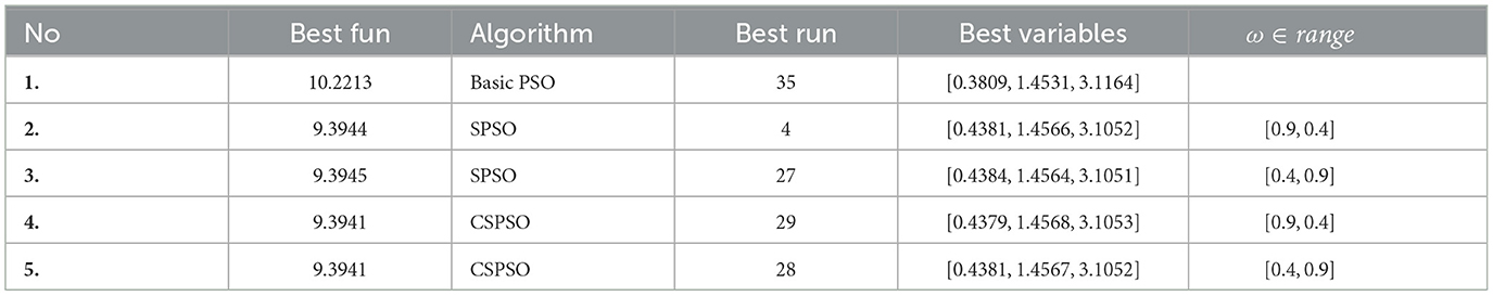
Table 1. Comparison of algorithms on optimization test functions.
The mean velocity vt+1 of (46) is shown using Table 1 and graphically (Figures 1–3) for the algorithms in Table 1. Figure 1 shows the convergence of PSO without controlling factor inertia weight exploded. One of the main limitations of PSO is that particles prematurely converge toward a local solution.
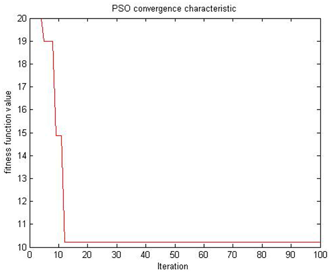
Figure 1. Basic PSO with no inertia weight for (46) on example 1.
The evaluation results of the compared algorithms are shown in Figures 2, 3 for decreasing and increasing inertia weight, respectively. Figure 2 shows the evolution of inertial weight of the compared algorithms over the running time. The main disadvantage is that once the inertia weight is decreased, the swarm loses its ability to search new areas [39]. Figure 3 shows the evolution of convergence characteristic for CSPSO based on inertial weight during the run. CSPSO can avoid premature convergence by performing efficient exploration that can help to find better solutions as the number of iterations increases and can avoid premature convergence by balancing exploration and exploitation. The algorithm CSPSO has shown fast convergence speed on unimodal functions.
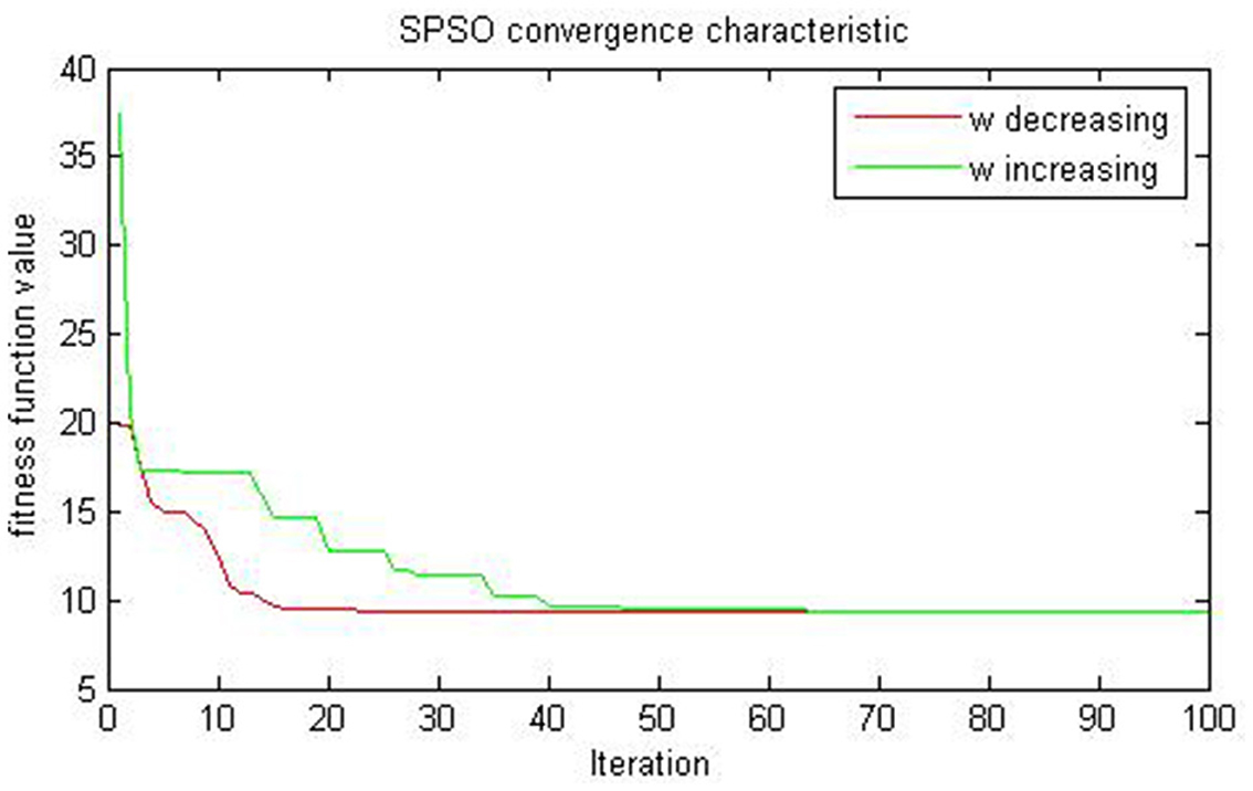
Figure 2. Evaluation of SPSO for (46) on example 1.
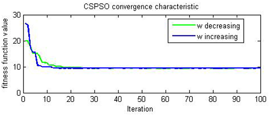
Figure 3. Evaluation of CSPSO for (46) on example 1.
In order to confirm the performance on multi-modal functions, we carry out a similar simulation by using (47).
The same set of parameters is assigned for all algorithms of Table 2 as in (46). Where in this function the number of local minima increases exponentially with the problem dimension. Its global optimum value is approximately −5.74, as we see from Table 2.
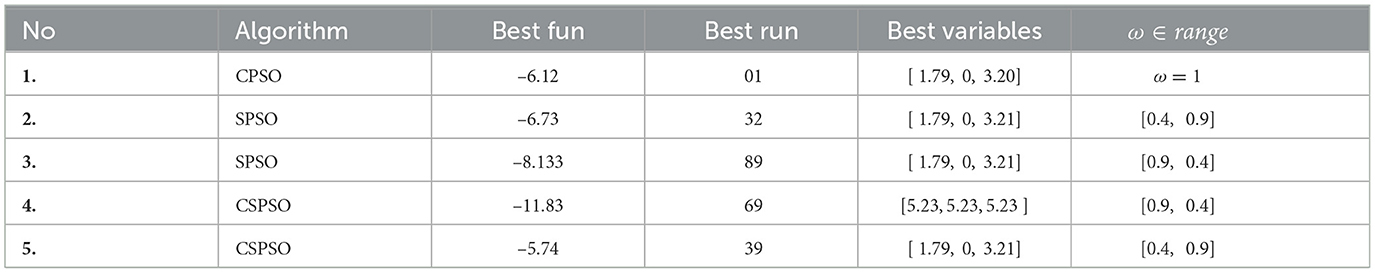
Table 2. Comparison of algorithms on optimization test functions of multi-modal.
Figures 4, 5 are simulations obtained from Table 2 results, and all the figures meet the objective of the CSPSO algorithm for the optimization problem given in (47) and its evaluation in Figure 6.
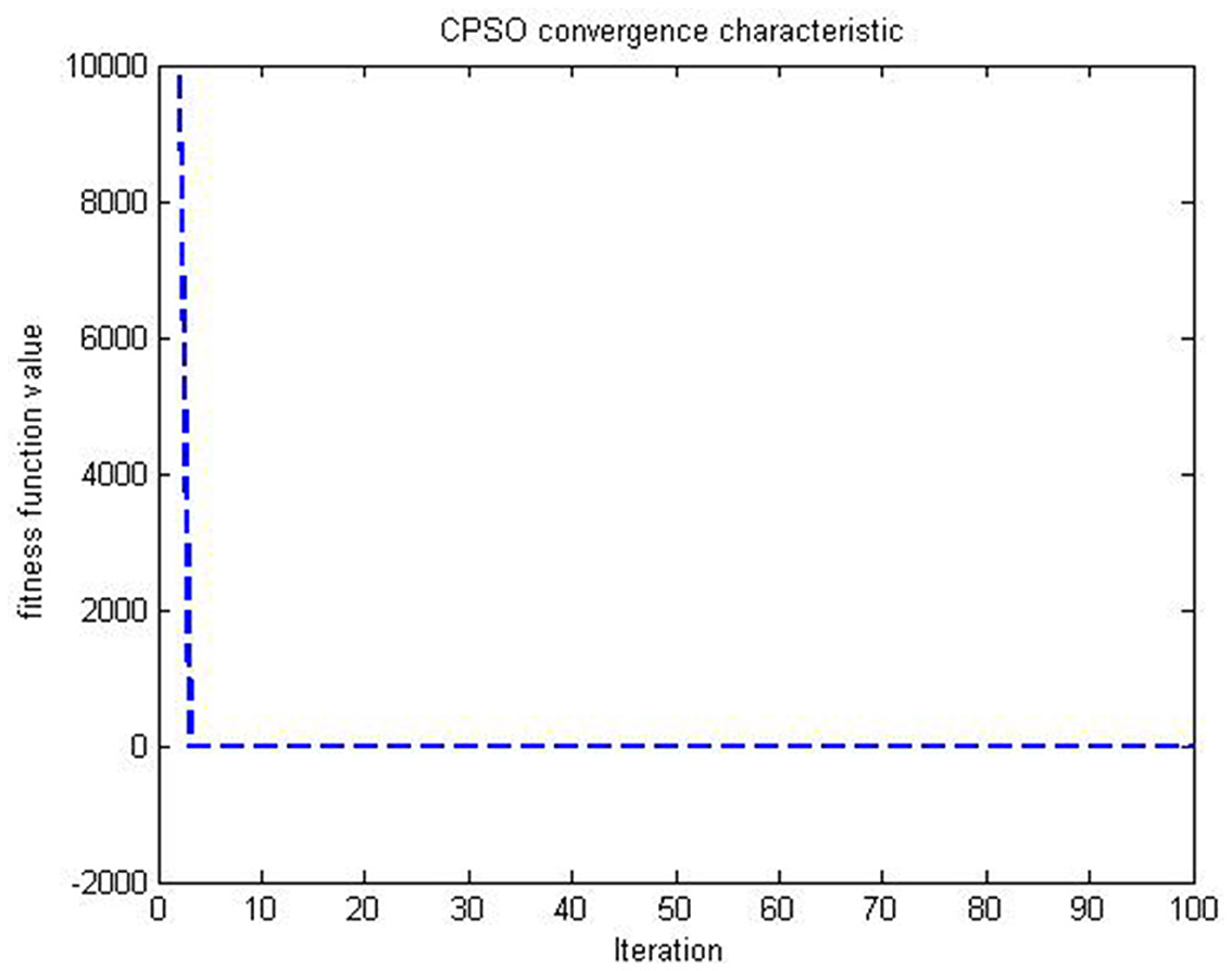
Figure 4. CPSO when ω = 1 for (47) on example 2.
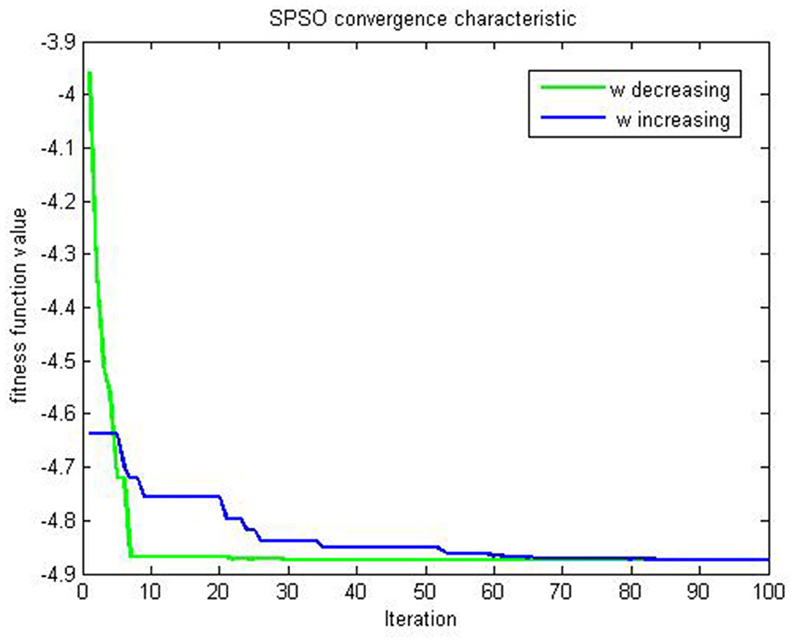
Figure 5. Evaluation of SPSO for (47) on example 2.
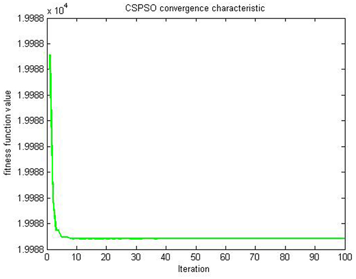
Figure 6. Evaluation of CSPSO for (47) on example 2.
5 Conclusion
This article mainly concerns the convergence and stability analysis of the CSPSO algorithm and its performance improvement for different constriction coefficients. We first investigated the convergence of the SPSO algorithm by relating it to the Markov chain in which the stochastic process and Markov properties employ quantum behaviors to improve the global convergence and prove Markov chain transition probability, showing that the CSPSO algorithm converges to the global optimum in probability. We also compared the proposed algorithm with basic PSO, SPSO, and CPSO algorithms evaluating the optimal value (fitness value) based on the range of ω. The proposed algorithm is fast and efficient, and the run plans of CSPSO for ω linearly decreasing from 0.9 to 0.4 are easy to implement. The CSPSO algorithm performs better because it regenerated those results to minimize the test functions. On the other hand, the proposed heuristic algorithm did not seek solutions that minimized the delay time or cost function, and the adjustment process would be stopped if no ω was identified as regular. The CSPSO algorithm is verified to be a global convergent algorithm. These promising results motivate other researchers to apply CSPSO to solve optimization problems. And in the future we will make further investigations on convergence and stability of PSO variants.
Data availability statement
The original contributions presented in the study are included in the article/supplementary material, further inquiries can be directed to the corresponding author.
Author contributions
DT: Formal analysis, Writing—original draft, Software, Investigation, Project administration. TG: Supervision, Methodology, Validation, Project administration, Writing—review & editing. SL: Conceptualization, Supervision.
Funding
The author(s) declare that no financial support was received for the research, authorship, and/or publication of this article.
Acknowledgments
Authors are grateful to the referees and handling editor for their constructive comments.
Conflict of interest
The authors declare that the research was conducted in the absence of any commercial or financial relationships that could be construed as a potential conflict of interest.
Publisher's note
All claims expressed in this article are solely those of the authors and do not necessarily represent those of their affiliated organizations, or those of the publisher, the editors and the reviewers. Any product that may be evaluated in this article, or claim that may be made by its manufacturer, is not guaranteed or endorsed by the publisher.
References
1. Kennedy J, Eberhart RC. Particle swarm optimization. In: Proceedings of the IEEE International Conference on Neural Networks, (1995). p. 1942–1948.
2. Ahmed G. GadParticle swarm optimization algorithm and its applications: a systematic review. Arch Comput Methods Eng. (2022) 29:2531–61. doi: 10.1007/s11831-021-09694-4
3. Banks A, Vincent J, Anyakoha CA. A review of particle swarm optimization. Part I: background and development. Nat Comput. (2007) 6:467–84. doi: 10.1007/s11047-007-9049-5
4. AlRashidi MR, El-Hawary ME. A survey of particle swarm optimization applications in electric power systems. IEEE Trans Evol Comput. (2009) 14:913–8. doi: 10.1109/TEVC.2006.880326
5. Kumar A, Singh BK, Patro BD. Particle swarm optimization: a study of variants and their applications. Int J Comput Applic. (2016) 135:24–30. doi: 10.5120/ijca2016908406
6. Tarekegn D, Tilahun S, Gemechu T. A review on convergence analysis of particle swarm optimization. Int J Swarm Intell Res. (2023) 14:328092. doi: 10.4018/IJSIR.328092
7. Clerc M, Kennedy J. The particle swarm-explosion, stability and convergence in a multidimensional complex space. IEEE Trans Evol Comput. (2002) 6:58–73. doi: 10.1109/4235.985692
8. van den Bergh F, Engelbrecht AP. A study of particle swarm optimization particle trajectories. Inform Sci. (2006) 178:937–71. doi: 10.1016/j.ins.2005.02.003
9. Kadirkamanathan V, Selvarajah K, Fleming PJ. Stability analysis of the particle dynamics in particle swarm optimizer. IEEE Trans Evol Comput. (2006) 10:245–55. doi: 10.1109/TEVC.2005.857077
10. Liu QF. Order-2 stability analysis of particle swarm optimization. Evol Comput. (2015) 23:187–216. doi: 10.1162/EVCO_a_00129
11. Dong WY, Zhang RR. Order-3 stability analysis of particle swarm optimization. Inf Sci. (2019) 503:508–20. doi: 10.1016/j.ins.2019.07.020
12. Jiang M, Luo YP, Yang SY. Stochastic convergence analysis and parameter selection of the standard particle swarm optimization algorithm. Inform Process Lett. (2007) 102:8–16. doi: 10.1016/j.ipl.2006.10.005
13. Poli R, Langdon WB. Markov chain models of bare-bones particle swarm optimizers. In: Proceedings of the 9th Annual Conference on Genetic and Evolutionary Computation. (2007). p. 142–149. doi: 10.1145/1276958.1276978
14. Cai ZQ, Huang H, Zheng ZH, Luo W. Convergence improvement of particle swarm optimization based on the expanding attaining-state set. J Huazhong Univ Sci Technol. (2009) 37:44–7.
15. Solis F, Wets R. Minimization by random search techniques. Math Oper Res. (1981) 6:19–30. doi: 10.1287/moor.6.1.19
16. van den Bergh F, Petrus Engelbrecht A. A convergence proof for the particle swarm. Optimiser Fund Inform. (2010) 105:341–74. doi: 10.3233/FI-2010-370
17. Dirk S, Carsten W. Runtime analysis of a binary particle swarm optimizer. Theor Comput Sci. (2010) 411:2084–100. doi: 10.1016/j.tcs.2010.03.002
18. Sun J, Wu X, Palade V, Fang W, Lai CH, Xu W. Convergence analysis and improvements of quantum-behaved particle swarm optimization. Inf Sci. (2012) 193:81–103. doi: 10.1016/j.ins.2012.01.005
19. Per KL, Carsten W. Finite first hitting time versus stochastic convergence in particle swarm optimization. Adv Metaheur. (2013) 53:1–20. doi: 10.1007/978-1-4614-6322-1_1
20. Yuan Q, Yin G. Analyzing convergence and rates of convergence of particle swarm optimization algorithms using stochastic approximation methods. IEEE T Automat Contr. (2015) 60:1760–73. doi: 10.1109/TAC.2014.2381454
21. Ren ZH, Wang J, Gao Y. The global convergence analysis of particle swarm optimization algorithm based on Markov chain. Control Theory Applic. (2011) 28:462–6.
22. Xu G, Yu G. On convergence analysis of particle swarm optimization algorithm. J Comput Appl Math. (2017) 333:65–73. doi: 10.1016/j.cam.2017.10.026
23. Feng P, Xiao-Ting LI, Qian ZH, Wei-Xing LI Qi GA. Analysis of standard particle swarm optimization algorithm based on Markov Chain. Acta Autom Sinica. (2013) 39:381–9. doi: 10.1016/S1874-1029(13)60037-3
24. Sun J, Feng B, Xu WB. Particle swarm optimization with particles having quantum behavior. In: Proceedings of the 2004 Congress on Evolutionary Computation, CEC04, Portland, USA (2004). p. 326–331.
25. Shi YH, Eberhart RC. Empirical study of particle swarm optimization. In: Proceedings of the Congress on Evolutionary Computation, (1999). p. 1945–1950.
26. Kennedy J. Bare bones particle swarms. In: Proceedings of the 2003 IEEE Swarm Intelligence Symposium, IEEE (2003). p. 80–87.
27. Kennedy J, Mendes R. Population structure and particle swarm performance. In: Proceedings of the Congress on Evolutionary Computation. (2002). p. 1671–6.
28. Liang JJ, Suganthan PN. Dynamic multi-swarm particle swarm optimizer. In: Proceedings of the IEEE Swarm Intelligence Symposium. (2005). p. 124–129.
29. Parrott D, Li X. Locating and tracking multiple dynamic optima by a particle swarm model using speciation. IEEE Trans Evol Comput. (2006) 10:440–58. doi: 10.1109/TEVC.2005.859468
30. Brits R, Engelbrecht AP, van den Bergh F. Locating multiple optima using particle swarm optimization. Appl Math Comput. (2007) 189:1859–83. doi: 10.1016/j.amc.2006.12.066
31. Zhao X. A perturbed particle swarm algorithm for numerical optimization. Appl Soft Comput. (2010) 10:119–24. doi: 10.1016/j.asoc.2009.06.010
32. Tang Y, Wang ZD, Fang JA. Feedback learning particle swarm optimization. Appl Soft Comput. (2011) 11:4713–25. doi: 10.1016/j.asoc.2011.07.012
33. Wang HF, Moon I, Yang SX, Wang DW. A memetic particle swarm optimization algorithm for multimodal optimization problems. Inform Sci. (2012) 197:38–52. doi: 10.1016/j.ins.2012.02.016
34. Huang H, Qin H, Hao Z, Lim A. Example-based learning particle swarm optimization for continuous optimization. Inform Sci. (2012) 182:125–38. doi: 10.1016/j.ins.2010.10.018
35. Lawler GF. Introduction to Stochastic Processes, second edition. London: Chapman and Hall/CRC Press. (2006).
36. Xiao XY, Yin HW. Moment convergence rates in the law of logarithm for moving average process under dependence. Stochastics. (2014) 86:1–15. doi: 10.1080/17442508.2012.748057
37. Hu D, Qiu X, Liu Y, Zhou X. Probabilistic convergence analysis of the stochastic particle swarm optimization model without the stagnation assumption. Inf Sci. (2021) 547:996–1007. doi: 10.1016/j.ins.2020.08.072
38. Chen J, Xin B, Peng Z, Dou L, Zhang J. Optimal contraction theorem for explorationexploitation tradeoff in search and optimization. IEEE Trans Syst Man Cybern Part A. (2009) 39:680–91. doi: 10.1109/TSMCA.2009.2012436
39. Ezugwu AE, Agushaka JO, Abualigah L, Mirjalili S, Gandomi AH. Prairie dog optimization algorithm. Neural Comput Applic. (2022) 34:20017–65. doi: 10.1007/s00521-022-07530-9
40. Lee J, Mukerji T. Probabilistic Particle Swarm Optimization (Pro]PSO) for Using Prior Information and Hierarchical Parameters. Department of Energy Resources Engineering, Stanford University (2014).
41. Schmitt M, Wanka R. Particle swarm optimization almost surely finds local optima. Theor Comput Sci. (2014) 561:57–72. doi: 10.1016/j.tcs.2014.05.017
Appendix
Matlab codes
tic
clc
clear all
close all
rng default
LB=[0 0 0]; UB=[10 10 10];
m=3; n=50;
wmin=0.9; wmax=0.4; c1=2; c2=2;
maxite=100; maxrun=100;
for run=1:maxrun
run
for i=1:n
for j=1:m
x0(i,j)=round(LB(j) + (UB(j)-LB(j))*rand());
end
end
x=x0; v=0.1*x0; for i=1:n
f0(i,1)=ofun(x0(i,:));
end
pbest=x0;
[fmin0,index0]=min(f0);
gbest=x0(index0,:);
ite=1;
tolerance=1;
rho=0.9;
while ite <= maxite && tolerance > 10−12
w =wmax-(wmax-wmin)*ite/maxite; kappa=1; phi1=2.05; phi2=2.05;
phi=phi1+phi2;
chi = 2*kappa/abs(2−phi−sqrt(phi2 − 4*phi));
a=1/w;
for i=1:n
for j=1:m
v(i,j)=chi*[w*v(i,j)+c1*rand()*(pbest(i,j)-x(i,j))+c2*rand()*(gbest(1,j)-x(i,j))];
end
end
for i=1:n
for j=1:m
x(i,j)=x(i,j)+v(i,j);
end
end
for i=1:n
for j=1:m
if x(i,j)<LB(j)
x(i,j)=LB(j);
elseif x(i,j)>UB(j)
x(i,j)=UB(j);
end
end
end
for i=1:n
f(i,1)=ofun(x(i,:));
end
for i=1:n
if f(i,1)<f0(i,1)
pbest(i,:)=x(i,:);
f0(i,1)=f(i,1);
end
end
[fmin,index]=min(f0);
ffmin(ite,run)=fmin;
ffite(run)=ite;
if fmin<fmin0
gbest=pbest(index,:);
fmin0=fmin;
end
if ite>100;
tolerance=abs(ffmin(ite-100,run)-fmin0);
end
if ite==1;
disp(sprintf('Iteration Best particle objective fun'));
end
disp(sprintf('
ite=ite+1;
end
gbest;
fvalue=-x(1)*sin(sqrt(abs(x(1))))-x(2)*sin(sqrt(abs(x(2))))-x(3)*sin(sqrt(abs(x(3))));
fff(run)=fvalue;
rgbest(run,:)=gbest;
disp(sprintf('——–'));
end
disp(sprintf(”));
disp(sprintf('************'));
disp(sprintf('Final Results——'));
[bestfun, bestrun] = min(fff)
bestvariables = rgbest(bestrun, :)
disp(sprintf('**********'));
toc
plot(ffmin(1:ffite(bestrun),bestrun),'–b','linewidth',2);
xlabel('Iteration ');
ylabel('fitness function value');
title('CSPSO convergence characteristic')
Keywords: PSO algorithms, convergence and stability, constriction factor, Markov chain, Monte Carlo
Citation: Tarekegn Nigatu D, Gemechu Dinka T and Luleseged Tilahun S (2024) Convergence analysis of particle swarm optimization algorithms for different constriction factors. Front. Appl. Math. Stat. 10:1304268. doi: 10.3389/fams.2024.1304268
Received: 29 September 2023; Accepted: 18 January 2024;
Published: 14 February 2024.
Edited by:
Guillermo Huerta Cuellar, University of Guadalajara, MexicoReviewed by:
Hector Eduardo Gilardi Velazquez, Universidad Panamericana, MexicoFelipe Medina-Aguayo, Instituto Tecnológico Autónomo de México, Mexico
Copyright © 2024 Tarekegn Nigatu, Gemechu Dinka and Luleseged Tilahun. This is an open-access article distributed under the terms of the Creative Commons Attribution License (CC BY). The use, distribution or reproduction in other forums is permitted, provided the original author(s) and the copyright owner(s) are credited and that the original publication in this journal is cited, in accordance with accepted academic practice. No use, distribution or reproduction is permitted which does not comply with these terms.
*Correspondence: Dereje Tarekegn Nigatu, dGVrZ2VtQHlhaG9vLmNvbQ==