 Lara Kassab1
 Alona Kryshchenko2
 Hanbaek Lyu3*Denali Molitor1
 Deanna Needell1
 Elizaveta Rebrova4
 Jiahong Yuan3
- 1Department of Mathematics, University of California, Los Angeles, Los Angeles, CA, United States
- 2Department of Mathematics, California State University Channel Islands, Camarillo, CA, United States
- 3Department of Mathematics, University of Wisconsin - Madison, Madison, WI, United States
- 4Department of Operations Research and Financial Engineering, Princeton University, Princeton, NJ, United States
Temporal text data, such as news articles or Twitter feeds, often comprises a mixture of long-lasting trends and transient topics. Effective topic modeling strategies should detect both types and clearly locate them in time. We first demonstrate that nonnegative CANDECOMP/PARAFAC decomposition (NCPD) can automatically identify topics of variable persistence. We then introduce sparseness-constrained NCPD (S-NCPD) and its online variant to control the duration of the detected topics more effectively and efficiently, along with theoretical analysis of the proposed algorithms. Through an extensive study on both semi-synthetic and real-world datasets, we find that our S-NCPD and its online variant can identify both short- and long-lasting temporal topics in a quantifiable and controlled manner, which traditional topic modeling methods are unable to achieve. Additionally, the online variant of S-NCPD shows a faster reduction in reconstruction error and results in more coherent topics compared to S-NCPD, thus achieving both computational efficiency and quality of the resulting topics. Our findings indicate that S-NCPD and its online variant are effective tools for detecting and controlling the duration of topics in temporal text data, providing valuable insights into both persistent and transient trends.
1 Introduction
Dynamic topic modeling investigates how latent themes emerge, evolve, and fade in temporal text datasets. Several works have examined topics and their evolution through time [1–4] using probabilistic models [1, 5], nonnegative matrix factorizations [6–8], and deep learning models [9]. For large and noisy datasets, such as social networks or news feed datasets, for the sake of interpretability, topic modeling techniques do not aim to recover all the topics, but only a subset of important topics. This raises a question of topic selection: What do we view as important? Motivated by this perspective, we propose dynamic topic modeling methods that can influence what kind of topics we recover. While some major topics may persist for an extended period of time, detecting short-lasting topics, that correspond to shorter-lasting, but impactful events or discussions, or seasonally trending periodic topics, could be as important. In this paper, we show that tensor-based methods are able to discover topics of variable persistence automatically. Moreover, we propose and compare two approaches to control the length of discovered topics, based on data chunking and on sparse decompositions. We construct a semi-synthetic dataset based on the 20 Newsgroups dataset [10] to serve as a simple and well-understood experiment and real-world data based on the ABC news headlines dataset [11].
The two most popular classic techniques for topic modeling are Latent Dirichlet Allocation (LDA) [12] and Nonnegative Matrix Factorization (NMF) [13, 14]. In LDA, one models a topic by a probability distribution on the set of words, which are evolved according to a Bayesian scheme by feeding in the batches of a (words×documents) matrix to receive (words×topics) and (topics×documents) representations [1, 15]. NMF is also a matrix-based method which decomposes the (words×documents) matrix into (words×topics) and (topics×documents) matrices. When the documents have timestamps, that is, ordered in time, the (topics×documents) matrix provides temporal ordering to the automatically detected topics. However, one can note that given a large amount of time-stamped documents, such as news articles or tweets, topic evolution frequently happens not from one document to the next in time, but rather from a batch of nearly simultaneous documents to the next. For example, two consecutive tweets coming from two different users likely have no relation to each other. This suggests naturally multi-order, or tensorial, structure of large streams of temporal data.
Tensor decompositions have many applications in machine learning [16, 17] including temporal analysis such as discovering patterns [18], discovering time-evolving topics [19, 20], predicting evolution [21] and more. Here, we focus on one of the most natural low-rank tensor decompositions based on CP-tensor rank, see, e.g., [16]. Recent prior work successfully employed nonnegative CP tensor decomposition for the discovery of temporal topics in text data [22, 23]. One can encode the entire corpus of documents as a 3-dimensional tensor where the three modes correspond to words, relatively simultaneous documents, and time, respectively. This way, the time dimension of the tensor is designed to focus on temporal changes in the aggregated information from one-time slice to the next.
We believe the role of nonnegativity constraint on the temporal mode is crucial for the NCPD-type methods to be able to detect both long-lasting and short-lasting topics. Indeed, NMF is well-known to be able to extract spatially localized features when applied to image data [13] by using nonnegativity constraints on the spatial mode. Being a 3D analog of NMF, NCPD should be able to extract spatio-temporally localized features, which correspond to “short-lasting” (temporally localized) “topics” (spatially localized features) in our context of dynamic topic modeling. While nonnegative factorizations are used ubiquitously for topic identification and interpretability, there is less work that makes use of NCPD for this purpose, especially in terms of localization in the time domain, making it ever more important to study the differences in output when using a matrix versus a tensor factorization method with temporal data.
Dynamic topic models based on Bayesian approach has been widely used in the literature, including the LDA-based method by Blei and Lafferey [1] and the Probit-Dirichlet hybrid allocation (PDHA) model by Lu [24] for detecting cyclical dynamics for short term topics, and the continuous-time dynamic topic model by Wang et al. [5]. These existing Bayesian methods typically do not study the comparative prevalence of several distinct topics through time but rather discover the topics that themselves change (or evolve through time).
NCPD has recently been used as a tool for dynamic topic modeling in the literature. Correia et al. [25] used NCPD for detecting time-evolving topics in legal precedent relevance topics, while Zhao et al. [26] used it for detecting time-evolving phenotype topics. Ahn et al. [27]. investigated robustness of NCPD as a dynamic topic modeling tool in terms of noise in the observed data and noise and overestimation of topic numbers. However, there is a lack of analysis of detecting short-lasting topics, proposing parameter choices for such detection (e.g., [20]), or developing a method for detecting topics of targeted temporal structures. Also, most past studies using NCPD for dynamic topic modling do not provide theoretical analysis of the proposed algorithms.
Our key insight in this work is to enforce sparseness constraints on the temporal factor matrix of NCPD as a means to control the temporal structure of the desired topics to be learned from a time-stamped text data. This idea has been inspired by the sparseness-constrained NMF proposed by Hoyer [28].
1.1 Contributions
While we find that NCPD is able to learn topics of various temporal structures, there is no means to “control” the type of temporal structures of the topics that we desire to learn. To overcome this difficulty, we propose a new method of NCPD that forces one of the factor matrices (specifically, the (time×topic) factor) to have a prescribed level of sparseness of its columns. We call this method the sparsity-constrained NCPD (S-NCPD). We propose a block-coordinate-descent-type algorithm that approximately finds such decomposition. Furthermore, inspired by the online NCPD algorithm in [23], we also propose an online version of the S-NCPD algorithm that iteratively factorizes a sequence of smaller tensors while enforcing the same sparseness constraint as in S-NCPD. Our algorithm for OS-NCPD follows the framework of stochastic regularized majorization-minimizaiton [29]. We experimentally validate that the proposed methods can successfully detect topics of desired temporal structure in real-world dynamic text data. Our contributions are summarized below.
• We demonstrate that NCPD is able to automatically detect and accurately represent topics of variable persistence from temporal text data.
• We propose Sparsity-constrained NCPD (S-NCPD) that actively controls the persistence of topics through constraining the sparseness of the columns of the (time×topic) factor matrix.
• We also propose an online version of S-NCPD (OS-NCPD), which has the same ability to control the persistence of learned topics as S-NCPD but is computationally more efficient than S-NCPD.
• We introduce α-effective length and normalized AUC metric for quantitative measures for topic lengths. Using these measures, we validate that S-NCPD and OS-NCPD successfully detect topics of desired persistence in real-world data.
1.2 Related work
Several works have examined topics and their evolution through time using probabilistic models [1, 5], nonnegative matrix factorizations [6–8], and deep learning models [9]. In Blei and Lafferty [1], propose a family of probabilistic time series models to analyze the time evolution of topics in large document collections. The model assumes that a discrete-time state space model governs the evolution of the natural parameters of the multinomial distributions that represent the topics. In Wang et al. [5], the authors propose a continuous time dynamic topic model which uses Brownian motion to model latent topics through a sequential collection of documents, where a “topic” is a pattern of word use that is expected to evolve over the course of the collection. Neither paper studies the prevalence of topics through time provides analysis on detecting short-lasting topics or proposes parameter choices for such detection. We also note that one of the advantages of NCPD and NMF over existing LDA methods is that there are far fewer parameter choices involved in the modeling process.
Tensor decomposition techniques have numerous applications in machine learning [16, 17] including temporal analysis such as discovering patterns [18], discovering time-evolving topics [19, 20], predicting evolution [21], modeling the behaviors of drug-target-disease interactions [30], and spotting anomalies [31]. More recent related work in the line of research includes [32–34]. However, there is a lack of analysis of detecting short-lasting topics or proposing parameter choices for such detection (e.g., [20]).
In Ahn et al. [22], the authors demonstrate NCPD as a dynamic modeling technique where critical temporal information is preserved, and events such as topic evolution, emergence, and fading are significantly easier to identify compared to NMF-based methods. There are recent empirical studies on dynamic topic modeling using NCPD by Correia et al. [25] and Zhao et al. [26].
While NMF can yield sparse nonnegative basis [13], such a sparseness is an indirect byproduct of the nonnegativity constraint and can be observed mostly when the feature vectors are well-aligned. In order to circumvent this issue, Hoyer proposed a sparseness-constrained NMF that can actively control sparseness [defined through a function of the ratio of the L1 and L2 norms, see (2)] by using and additional projection step between alternatively optimizing the factor matrices [28], without providing any convergence guarantee of the proposed optimization algorithm.
Heiler and Schnörr observed that Hoyer's sparseness-constrained NMF can be viewed as a second-order cone programming [35] with bi-convex constraint along with additional reverse-convex constraints. Algorithms to find global optimum of convex programs with additional reverse-convex constraint has been studied by Tuy [36]. Based on this work, the authors proposed an alternative algorithm (called the sparsity maximization alg.) for solving sparseness-constrained NMF with a first-order stationary point guarantee. The authors also extended this approach to NCPD with sparseness constraint and showed that a natural extension of the sparsity maximization algorithm also produces stationary points asymptotically [37]. Our sparseness-constrained NCPD is closely related to the study in Heiler and Schnorr [37]. For theoretical analysis of a proposed algorithm, we also use the general convergence and complexity analysis for block majorization-minimization in Lyu and Li [38].
In this work, we provide an online variant of the sparseness-constrained NCPD for effective computation of the sparsity-controlled dynamic topics. The model formulation as an expected loss minimization and the proposed algorithm is inspired by the study on online NCPD by Lyu et al. [23]. For the convergence analysis of the proposed online algorithm, we use the general framework of stochastic regularized majorization-minimiation by Lyu [29].
1.3 Preliminaries and notation
We denote vectors with lowercase letters x with x(k) denoting its kth entry, matrices with uppercase boldface letters, X, and third-order tensors with uppercase calligraphic letters . Tensors are common algebraic representations for multidimensional arrays. The order of a tensor is the number of dimensions, which is also referred to as ways or modes [16]. For a matrix X, the vector xk denotes its kth column. We let ||·||F and ||·||1 denote the entrywise Frobenius norm, and the entrywise L1 norm respectively. The set of nonnegative real numbers [0, ∞) is denoted ℝ≥0. We let ⊗ denote the outer product of two vectors. For tensors and of the same size, denote by the Hadamard (pointwise) product. When B is a matrix, for each 1 ≤ j ≤ n, we denote their j-mode product by . See Kolda and Bader [16] for an excellent survey of related definitions and tensor algorithms. The notation is the variant of “big-O” notation that ignores the logarithmic factors.
1.4 Organization
In Section 2.1, we first introduce standard dynamic topic modeling methods: latent Dirichlet allocation (LDA), nonnegative matrix factorization (NMF), and nonnegative CP tensor decomposition (NCPD). Then we introduce sparsity-constrained NCPD (S-NCPD) and online S-NCPD as well as algorithms for solving the corresponding optimization problems. In Section 2.2, we introduce quantitative measures of the topic length. In Section 4, we analyze the performance of various dynamic topic modeling methods, including existing ones and the two newly proposed ones. Our focus is on the type of temporal structures of the topics learned by each method. We use semi-synthetic and real datasets in our experiments. Lastly, we include some discussions regarding those techniques and their results.
2 Materials and methods
2.1 Tensor factorization methods for topic modeling
In this section, we discuss NMF, NCPD, and an online version of NCPD.
2.1.1 Nonnegative matrix factorization
Nonnegative Matrix Factorization (NMF) is a popular tool for extracting hidden themes from text data [41, 42]. For a data matrix , one learns a low-rank dictionary and code matrix that minimize , where r>0 is typically chosen such that r < min{m, n}. Suppose m denotes the number of features (in our case unigrams and bigrams) and n the number of documents, then the dictionary matrix W represents topics in terms of the original features. Each column of the code matrix H represents a data point as a linear combination of the dictionary elements with nonnegative coefficients. We use NMF to learn a dictionary W from all data and analyze topic dynamics through changes in topic prevalence over time in the code matrices from each time slice.
2.1.2 Latent Dirichlet Allocation
Latent Dirichlet Allocation (LDA) is another popular tool for extracting hidden topics from text data [12]. LDA is a hierarchical Bayesian model, in which words and documents are modeled as a finite mixture over an underlying set of topics. For each topic k, let βk be a multinomial distribution over the vocabulary which is assumed to have been drawn from a Dirichlet distribution Dirichlet(η). For each document d, let θd be a distribution over topics that are assumed to have Dirichlet prior Dirichlet(α). These prior distributions are assumed to be symmetric. LDA then updates the prior distributions of β and θ and approximates posterior distributions. Two approaches are commonly used to approximate posterior distributions Markov Chain Monte Carlo (MCMC) methods and variational inference.
In our experiments, we consider an LDA model that uses online variational inference [15]. The posterior distribution of β is used to find word representation of each topic and the posterior distribution of θ gives the topic distribution for each document. To learn topic dynamics over time, we take the mean over topic distributions θi for all the documents in each time slice and present them as columns of the heatmaps (e.g., Figure 5).
2.1.3 Nonnegative CP tensor decomposition
Nonnegative CP Tensor Decomposition (NCPD) is a tool for decomposing higher-dimensional data tensors into interpretable lower-dimensional representations. NCPD factorizes a tensor into a sum of nonnegative component rank-one tensors, defined as outer products of nonnegative vectors [39, 40]. For instance, given a third-order tensor and a fixed integer r>0, the approximate NCPD of seeks matrices , such that where the nonnegative vectors ak, bk, and ck are the columns of A, B, and C, respectively. The matrices A, B, and C are referred to as the NCPD factor matrices. Such factor matrices are found by solving the following minimization problem
NCPD for decomposing any dth order data tensor can be formulated similarly. Nonnegative Matrix Factorization (NMF) is a special instance of NCPD for decomposing second-order tensor data, which is a popular tool for extracting hidden themes from text data [41, 42].
Note that (1) is a non-convex optimization problem, but the objective function ℓ in (1) is block multi-convex (i.e., convex in each factor matrix while the other two factors are held fixed). Leveraging this structure, many researchers proposed algorithms for solving (1) have the nature of block coordinate descent (BCD) [43, 44], including the multiplicative update algorithm [45], alternating least squares [39, 40]. Recently, Lyu and Li showed that regularized versions of these algorithms converge to the set of stationary points and can produce an ϵ-stationary point of the objective in (1) within iterations [38].
NCPD is considered a topic modeling technique for tensor data that successfully showcases topic variation across all modes of the tensor [including temporal mode(s)] [22]. Namely, suppose we have a third-order tensor data where n1 = words denotes the number of words in the vocabulary, n2 = batch denotes the number of documents in a time slice, and n3 = time denotes the number of time slices. Applying NCPD to the third-order tensor data , we obtain three factor matrices A, B, and C of shapes (words×r), (batch×r), and (time×r), respectively, where r = topics equals the number of topics we seek to find. We will be the most interested in the factor matrices A and C; the columns of A give r topics in the data whereas the corresponding columns of C give how their prevalence evolves through time. The second-factor matrix B gives information on specific groups of documents that contributed to each discovered topic, which is of less importance for our purpose of dynamic topic modeling.
2.1.4 Sparseness-constrained NCPD (S-NCPD)
In order to control the temporal prevalence of learned topics, we propose to restrict the structure of the (time×r) factor matrix C in NCPD as defined in Equation (1) so that its columns have a “prescribed value of sparseness”. For this, we use the following measure of the sparseness of a vector introduced in Hoyer [28] in the context of NMF: for a vector ,
As observed in [28], this is a smooth counterpart of ||x||0 function. Indeed, it interpolates between s(x) = 1 for x so that ||x||0 = 1 and s(x) = 1 if all the components of x are equal up to their signs.
Fix two parameters 0 ≤ ρmin ≤ ρmax ≤ 1. We propose the following sparseness-constrained NCPD (S-NCPD):
where f is as in (1) and Cj denotes the jth column of the (time×r) matrix C. Note that Cj describes the time evolution of the prevalence of the jth topic represented by the jth column A[:, j] of the (words×r) matrix A. Thus, the additional sparsity constraint on the columns of C in (3) actively controls the types of topics. We will typically use a single “temporal sparseness level” ρ = ρmin = ρmax. In this case, for large ρ we seek long-lasting topics, and for small ρ we prefer short-lasting topics. We remark that (3) is a tensorial extension of Hoyer's sparsity-constrained NMF [28], where the goal is to control the sparsity of the dictionary atoms learned by NMF. A similar model of NCPD with sparseness constraint on each factor has been considered by Heiler and Schnörr [37]. Our unique insight is that we use the enforced sparseness on the columns of the temporal factor as a way to control control the temporal structure of topics learned by NCPD.
Since the problem (3) also has a block multi-convex objective function, in order to compute an approximate optimum for the S-NCPD problem, we may use a modified version of alternating least squares (ALS) with proximal regularization of the following form:
The constraint on the temporal factor Ct in (4) is given by the intersection of the nonnegativity and sparseness constraints. The latter is the set of all vectors in with a fixed ratio between the L1- and L2-norms (depending on ρ), which is unfortunately not a convex constraint. Hence known theoretical results for block coordinate descent with convex constraints sets (e.g., [38]) do not apply, and we will need to compute an approximate solution for Ct. In order to do this, we use the projected-gradient-decent-type Algorithm 1 for sparseness-constrained nonnegative least squares.
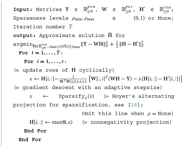
Algorithm 1. Sparseness-constrained nonnegative least squares (S-NLS).
In order to compute in (4), we use Algorithm 1 with the mode-3 unfolding of and whose columns are vectorization of the outer products of respective columns of At and Bt. Hoyer's alternating projection for sparsification [28] finds a nearby vector that approximately matches the desired sparseness level. Note that high (resp., low) values of ρ result in topics that have sparse (resp., dense) prevalence (e.g., columns of the (time×r) factor matrix). In order to compute the other two factors, At and Bt, we used Algorithm 1 with ρ = None.
We remark on the per-iteration computational complexity of Algorithm (4). In order to reformulate each of the three sub-problems in (4), we need total O(r(n1n2+n2n3+n1n3)) computation. Thereafter we apply Algorithm 1 for O(1) sub-iterations, where each gradient descent step with nonnegative projection takes computations. For sparsification, each step of Hoyer's alternating L1/L2-projection takes O(rni) computation, which we iterate only a fixed amount of times. Hence the total per-iteration complexity is .
2.1.5 Sparseness-constrained online nonnegative CP decomposition (OS-NCPD)
The computational cost of applying S-NCPD to a large 3D tensor may be computationally infeasible. Following the Online NCPD by Lyu et al. [23], here we propose an online version of S-NCPD that we call Online S-NCPD (OS-NCPD for short). This method is a mini-batch extension of the batch S-NCPD (3), where mini-batches of sub-3D tensors are processed in a sequential manner to progressively compute a (words×r) factor A and (time×r) factor C with column-wise sparseness constraint.
The key idea behind OS-NCPD is as follows. Recall that each temporal slice of the 3D tensor consists of multiple “simultaneous” documents in the time domain. In our application, extracting features from a batch of documents coming from the same time slice is not of major importance. So, what if on each time slice we subsample only a small number batch′≪batch of documents, and apply S-NCPD to the resulting smaller tensor of shape (words×batch′ × time)? This will give us three factor matrices A, B′, and C of shapes (words×r), (batch′ × r), and (time×r), respectively, where the first and last factor matrices A and C have the same shapes as before. While using S-NCPD on a single subsample of the original tensor has reduced computational cost, we may also lose some information since we only learn from a single subsample. However, it is possible to process a number of such subsamples in a sequential manner, so that each factorization problem has a reduced dimension but the factor matrices A and C improve over subsamples.
The OS-NCPD can be formulated by a stochastic program as follows. Given a probability distribution π on the set of data tensors , consider seeking nonnegative factor matrices and by solving the following stochastic program
where the random data tensor is sampled from the distribution π. The stochastic program (5) is equivalent to the S-NCPD problem (3) when the distribution π is supported on a single data tensor.
We propose the following iterative algorithm for solving (5), which is a minor modification for the Online CP-dictionary learning (OCPDL) algorithm in [23]. Suppose we have learned the loading matrices At−1, Ct−1 from the sequence of data tensors in . Then we compute the updated loading matrices [At, Ct] by
where λ≥0 is an absolute constant and (wt)t≥1 is a non-increasing sequence of weights in (0, 1]. The recursively defined function is called the surrogate loss function, which is quadratic in each factor A and C but is not jointly convex. Namely, when the new tensor data arrives, one computes the (batch′ × r) factor for with respect to the previous loading matrices in (At−1, Ct−1), updates the surrogate loss function , and then sequentially minimizes it to find updated loading matrices within diminishing search radius wt. In our implementation, for each t, we subsample a tensor of shape n1×n2×n3 from uniformly at random. During the execution of the algorithm, one only needs to store a matrix of dimension , regardless of the total number of iteration T. We refer the reader to [23] for more details.
In comparison to the original OCPDL algorithm, in (6) we added additional sparsity constraint on the columns of Ct. An approximate solution for Ct can be computed using a projected gradient descent method similar to Algorithm 1. The original OCPDL algorithm is guaranteed to almost surely converge to the set of stationary points of the objective of (5) and shows a superior convergence rate against standard (offline) algorithms for NCPD. Recently in [29], it was shown that this algorithm can produce an ϵ-approximate stationary point of the objective within iterations.
The per-iteration computational cost of ONCPD and OS-NCPD is , which is a factor improvement over that of their offline counterparts. This is due to the fact that at each iteration, we work with a subsampled tensor of size instead of the full tensor of size n1×n2×n3.
2.2 Quantifying lengths of topics
How can we determine the “length” of a topic found by any of the described methods? How can we judge whether a topic is considered “short-lasting” or “long-lasting”?
First, we can judge the topic lengths visually based on the heatmaps of matrix representing the dynamics of the topics over time where r denotes the number of topics and n number of time units or stamps. In the case of NCPD, S-NCPD, and OS-NCPD, T = C is a temporal factor matrix, and in the cases of NMF and LDA, the columns of T are topic intensities over the time slices. By construction, this matrix T has normalized columns. Qualitatively, approximately sparse rows of the matrix T correspond to the topics that were trending shortly or periodically.
To complement this qualitative analysis of the topics' lengths, in this section, we propose a metric to quantify the notion of the length of a topic. This way, one can explicitly parametrize the effective (approximate) length of each topic and demonstrate the variability of the topic lengths discovered by the tensor-based methods.
Our proposed metric quantifies the number of consecutive time units required to cover a certain “proportion” of the topic that we denote by α. We consider the matrix which is the matrix T with the rows normalized to add up to 1. Normalization of the rows produces a probability distribution for each individual topic over time. Informally, it captures how many consecutive time units are required for each topic to include a certain proportion of its whole “mass”. Specifically, for a fraction α∈[0, 1] and the topic τ, its α-effective length denoted by ℓα(τ), is defined as
By definition, for α = 0, all the topics will have zero length. For α = 1, the length of the topic is the total number of nonzero entries in the corresponding row. Typically, the intermediate values of α could demonstrate the variability of the topic lengths. The choice of parameter α can be determined by a specific application. Visually, this technique acts as an “elbow method” as α varies, where we can also observe the re-occurrence of a topic by the number of elbows in the curve.
By varying the value of α in [0, 1], one obtains plots of the function α↦lα(τ), which we refer to the topic ROC, from which various information on temporal features of learned topics can be extracted. We note the following elementary but useful observations on topic ROCs:
(a) The diagonal line in topic ROC corresponds to topics that are uniformly distributed over the entire time horizon;
(b) For any topic τ, its topic ROC lies beneath the diagonal line;
(c) If a topic τ is fully covered by k-consecutive time units, i.e., ℓ1(τ) = k, then its topic ROC lies beneath the line segments from (0, 0) to (1, k).
Based on the above observations, it is also possible to give a single persistence score for each topic, that is, a number independent of other parameters (such as α) and of visual judgment. One of many ways to define it is to aggregate the α-effective lengths with various values of α, measuring the area under the curve α↦lα(·), and normalizing it by 1/2 total number of time slices in the time range. Such normalization guarantees all the persistence (nAUC) scores to be in the range between 0 and 1, since the curve lα always lies under the diagonal. Indeed, nAUC equals 1 corresponds to the “most persistent” topic having equal weights at each time slice in the range [observation (a)]. Further, if a topic is fully covered by a short time interval, its nAUC score would be close to 0 [observation (c)].
We note that multiple variations of the definition (7) are possible and might be preferable in some applications. For example, the alternative measure that considers non-consecutive time unit contributions to the topic length would be able to detect periodic topics like the ones we can visually observe in topic 16 in Figure 7.
3 Theoretical analysis
In this section, we provide some theoretical analysis for the proposed algorithms (4, 6).
The challenging aspect in analyzing optimization algorithms for S-NCPD in (3) is that the additional sparseness constraint is nonconvex. In fact, such a nonconvex constraint set can be expressed by a convex set (for the max sparseness) and a reverse-convex set (for the min sparseness), as observed by Heiler and Schnörr [46]. The second order cone is the convex set [47]:
In order to analyze Hoyer's sparseness-constrained NMF [28], Heiler and Schnörr introduced the following family of convex sets
In [35], it was shown that, for 0 ≤ ρmin < ρmax ≤ 1,
That is, the set of all vectors in ℝn with sparseness at most ρmax is precisely the convex set defined above; Also imposing the minimum sparseness ρmin amounts to take the reverse-convex constraint (e.g., imposing its complement). Therefore, the problem of finding the sparseness-constrained temporal factor Ct in (4) as the following convex program with an additional reverse convex constraint:
Tuy [36] proposed algorithms that can provably find a global optimum of problems of the form above, where one seeks to minimize a convex function subject to a single convex set and a single reverse-convex set. As noted in [36], such methods incur a considerable computational cost. In order to handle such computational issues and also the multiple reverse-convex constraint as in (8), Heiler and Schnörr [46] proposed an alternative algorithm called the “sparsity maximization algorithm”. The idea is to first maximize the linearization of the sparseness measure subject to the constraint that the objective value must not increase; then, dualy, one minimizes the objective function under the condition that the min-sparsity constraint may not be violated. We refer to the details of the algorithm to ([46], Alg. 5.2). A minor modification of the analysis in [46] shows that a version of our modified ALS algorithm for S-NCPD converges to the set of stationary (first-order optimal) points.
Proposition 3.1. Suppose one solves (3) by the modified ALS algorithm 4 with positive proximal regularization (λ>0) and the sparseness maximization algorithm ([46], Alg. 5.2) for solving for the temporal factor Ct. Suppose 0 ≤ ρmin < ρmax ≤ 1. Then this algorithm converges asymptotically to the set of stationary points of (3).
Proof. This result follows from a minor modification of the proof of ([46], Prop. 10). There instead of using proximal regularization, one needs to assume that the objectives of the subproblems must stay positive definite throughout the iterations. We can omit this assumption by using proximal regularization as in (4) with λ>0.
Despite the nice theoretical properties of utilizing the sparsity maximization algorithm within our algorithm, such an algorithm involves solving two second-order cone programs [48] at each iteration. This could incur considerable computational burden when handling large tensors (e.g., our News Headlines of size 203 × 7, 000 × 700 in Section 4.3 compared to the MIT CBCL face data set of size 19 × 19 × 2429 used in [46]). Our Algorithm 1 is a faster alternative, which essentially implements block projected gradient descent that updates each column of a sparseness-constrained factor in multiple rounds. Due to the reverse-convex constraint as we discussed before, our theoretical guarantee for the ALS algorithm with Algorithm 1 used to compute the temporal factor Ct covers only the cases when either the max sparsity or the min sparsity constraints are trivial. However, in such special cases, we are able to obtain not only asymptotic convergence results but also a more practical iteration complexity result, as stated in Theorem 3.2 below.
Theorem 3.2 (Convergence and complexity of for S-NCPD). Suppose λ>0 and either ρmin = 0 or ρmax = 1. Consider the modified ALS algorithm (4) that uses Algorithm 1 with T = ⌊clogt⌋ iterations for computing the temporal factor Ct. If the constant c>0 is sufficiently large, then the algorithm converges asymptotically to the set of stationary points of the S-NCPD problem (3). Furthermore, it achieves an ϵ-stationary point within O(ϵ−2(logϵ−1)2) iterations.
Proof. Suppose without loss of generality that ρmin = 0. Then the subproblem for computing the temporal factor Ct becomes a convex program:
Note that Algorithm 1 implements T rounds of block projected gradient descent, where each column of Ct is a single block. By a straightforward computation, one can show that the largest eigenvalue of the Hessian of the regularized least squares objective in Algorithm 1 for the ith row of H is at most WTW[i, i]+λ. Thus the stepsize is guaranteed to be strictly less than the reciprocal of the Lipschitz constant for the corresponding block-gradient. Consequently, the objective value decays exponentially fast toward the global minimum due to the standard complexity result for block coordinate descent for strongly convex minimization [49] (here we need positive proximal regularization λ>0 for strong convexity). Thus by choosing c>0 large enough, Algorithm 1 converges to an approximate solution to (9) within a function value gap O(t−2) for each t. Consequently, the sub-optimality gaps at each iteration are summable for t≥0. This allows one to apply the general result on the convergence and complexity of block majorization-minimization in Lyu and Li ([38], Thm. 2.1). Then the result follows.
Lastly in this section, we discuss the convergence guarantee for the proposed algorithm for OS-NCPD in (6).
Theorem 3.3 (Convergence and complexity of for OS-NCPD). Suppose λ>0 and either ρmin = 0 or ρmax = 1. Consider the modified OCPDL algorithm 4 for OS-NCPD. Assume the weight sequence for some δ>0. Then, almost surely, the algorithm converges asymptotically to the set of stationary points of the OS-NCPD problem (5). Furthermore, it achieves an ϵ-stationary point within O(ϵ−4(logϵ−1)δ) iterations almost surely.
Proof. As before, note that the sparseness constraint set for the temporal factor Ct in (6) becomes convex under the hypothesis of ρmin = 0 or ρmax = 1. Thus the algorithm (6) falls under the framework of stochastic regularized majorization-minimization with multi-convex surrogate in Lyu [29]. Then the result follows from Theorem 4.1 and Corollary 4.5 in [29].
4 Experimental results
In this section, we compare the performance of NMF, LDA, NCPD, and ONCPD methods in identifying temporal topics in semi-synthetic and real datasets.
4.1 Experimental setup
In all the experiments, documents are converted to term frequency-inverse document frequency (TFIDF) vector representations using the sklearn TFIDFVectorizer [50]. We compute NMF of the data matrix using sklearn [50] with nonnegative double singular value decomposition initialization [51]. We compute NCPD of the tensor data with multiplicative updates [45] using TensorLy [52] and SVD initialization. We compute ONCPD using the Online CP-Dictionary Learning algorithm in [23] with SVD initialization. The subsampled batch size () for ONCPD (see Section 2.1.5) equals 5 for 20 Newsgroups (full batch = n2 = 26, see Section 4.2) and 100 for the Headlines dataset (n2 = 700, see Section 4.3). These values are chosen by cross-validation among 5%, 10%, 15%, and 20% of n2. For S-NCPD and OS-NCPD, we implemented algorithms 4 and 6, respectively, with Algorithm 1 with T = 5 to solve the sub-problems subroutine In our experiments. For the sparsity projection used in Algorithm 1, we used Hoyer's alternating projection algorithm [28] for 10 iterations. We did not find significant performance gain for more than 10 iterations for the alternating projection. All algorithms are ran up to 500 iterations with early stopping when the gradient norm is less than 1% of the norm of the data tensor. Lastly, for LDA we construct a bag-of-words corpus using the same dictionary as the other methods (obtained from the TFIDF weights) and compute the model using gensim LDA model [53] with various numbers of passes and training chunks to save memory on larger datasets [15].
The keyword representation of each of the extracted topics is also provided for interpretability. Each learned topic is represented by a positive linear combination of terms. Terms with larger values in a particular topic are more significant for that topic and, thus, the terms with the largest values provide interpretable descriptions of the topics. The number of topics for the synthetic 20 Newsgroups dataset is chosen to match the known number of article subjects. For complex real-world data, News Headlines datasets, we choose the number of topics to balance readability and the discovery of relevant events. We believe that increasing the number of topics could reveal additional relevant topics.
To quantify the interpretibility and coherence of the topics learned by various methods, we use the Cv score [54]. The Cv score is calculated based on co-occurrence statistics of words within a sliding window of a certain size in a reference corpus. It measures the coherence of a topic by considering the pairwise word co-occurrences within that window. The coherence score is higher if the words in a topic tend to co-occur more frequently within the reference corpus. In simpler terms, a higher Cv score indicates that the words in a topic are more closely related and thus the topic is more coherent and interpretable.
4.2 Semi-synthetic dynamic dataset results
The 20 Newsgroups dataset [10] is a collection of documents divided into six groups partitioned into subjects, with a total of 20 subtopics. This dataset is commonly used as an experimental benchmark for document classification and clustering. We consider a semi-synthetic dataset constructed from the 20 Newsgroups dataset to illustrate the dynamic topic modeling performance of NMF, LDA, NCPD, and ONCPD on a simple and well-understood dataset.
We consider only five categories: “Atheism”, “Space”, “Baseball”, “For Sale”, and “Windows X” with a total of 1,040 documents. We remove headers, footers, and quotes from all documents and compute TFIDF representation with a vocabulary size equal to 5,000. The NLTK English stopword list [55], and words appearing in more than 95% of the documents are removed. We organize the dataset into a 5000 × 26 × 40 tensor with dimensions: vocabulary size by number of documents by time. Each time slice consists entirely of articles from the same category, and the categories of the times slices are ordered as: (“Aethism”, time slices 1-2), (“Space”, time slices 3-20), (“Baseball”, time slices 21-23), (“For Sale”, time slices 24-35), (“Windows X”, time slices 36-37), and (“Baseball”, time slices 37-40). The tensor is illustrated in Figure 1. We run NMF, LDA, NCPD, and ONCPD as described in Section 2.1 with a rank equal to 5 reflecting the number of categories in the dataset. In this section, for NMF and LDA, we first unfold the tensor along the time mode, learn the topics, and then compute the mean topic representation for each time slice.
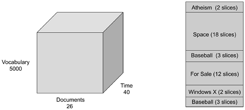
Figure 1. Semi-synthetic 20 Newsgroups tensor construction.
Learned topics and the prevalence of each topic over time are indicated for each method in Figure 2. On this semi-synthetic data, NCPD and ONCPD identify topics associated with each subject and accurately indicate the temporal occurrence of each subject, while NMF and LDA learn topics that are prevalent during time slices associated with multiple subjects. NCPD and ONCPD learn a single topic for each subject included in the dataset and accurately attribute the highest prevalence to the true underlying topic in each time slice. NMF and LDA also learn reasonable topics, including topics corresponding to the longer-lasting “Space” and “For Sale” segments. On this relatively simpler semi-synthetic data, NMF and LDA detect some but not all of the short-lasting topics. For example, NMF's learned topic 1 spikes in prevalence during the short-lasting “Aetheism” and “Baseball” segments, while LDA accurately detects a short-lasting “Windows X” related topic.
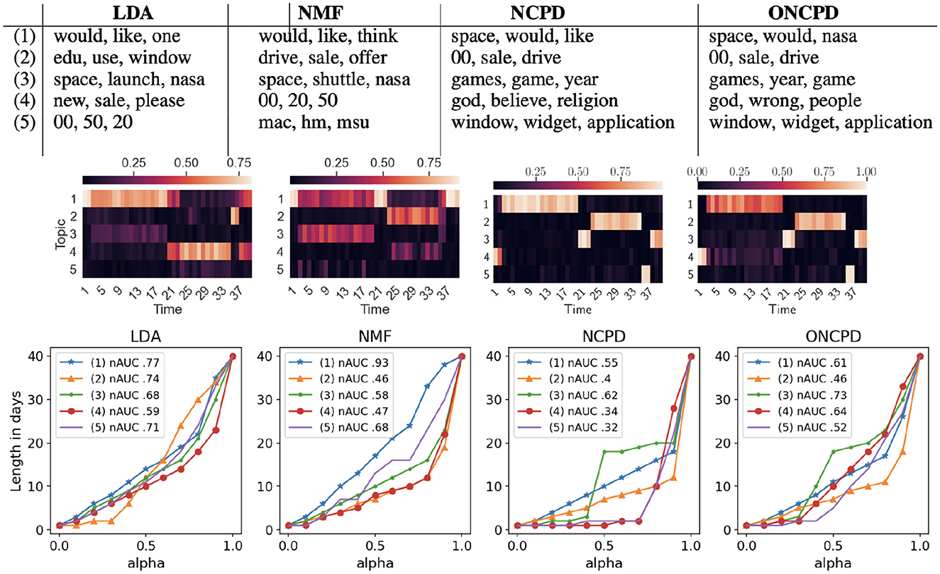
Figure 2. Top: three most important keywords corresponding to each of five topics learned from the semi-synthetic 20 Newsgroups dataset using four baseline models (LDA, NMF, NCPD, ONCPD). Middle: the learned topics and prevalence of each extracted topic. The columns of each heatmap indicate the distribution of the extracted topics for each time slice. Bottom: plot of the α-effective lengths of all 5 topics against α ∈ [0, 1] of the 20news dataset over LDA, NMF, NCPD, and ONCPD methods. The normalized area under the curve (nAUC) is given for each topic in the legend. Smaller nAUC scores indicate shorter-lasting topics, see Section 2.2.
Both LDA and NMF learn topics that blend multiple document subjects. For example, for both NMF and LDA, the most prevalent topic detected during the “Atheism” time slices is also present during the “Space” time slices. Indeed, we observe that the tensor-based method is able to better detect short-lasting topics and accurately represent them in time.
In Figure 2 (bottom), we track the effective lengths of each of 5 topics for a range of the values of α. The intermediate values of α~0.5 can show significant differences in the topic length variability across the methods. We can see that NCPD discovers 2 topics so that 70% of them appeared within 2 day period. One topic so that its 70% took 8 days and 2 more topics that require more than 15 days for their 70% of the content. In contrast, all the topics discovered by LDA have similar lengths and are generally longer than those discovered by NCPD: for the 70% of the content, all of them require at least a 12 daytime window.
With an elbow method, NCPD discovers two short-lasting topics (topics 4 and 5) with the 0.7-effective length of one day, two topics (topics 2 and 1) of 0.9-effective lengths of 10 and 18 days, respectively, and one topic (topic 3) of 0.9-effective length of 20 days that also has 0.4-effective length of only 2 days (which is, precisely the lengths of these artificially created topics). Choosing α in a shape-agnostic way, with α~0.5, we also see that only NCPD method finds 2 short-lasting topics with an effective length of one day and three longer topics with diverse lengths. The legends contain topic numbers referring to the table above, for example, topic (3) of the NMF has the top three words “space, shuttle, nasa”. Additionally, the normalized area under the curve (nAUC) is given for each topic in the legend. It is normalized to be one for a topic uniformly distributed over time. Thus, nAUC shows the persistence of topics by aggregating the α-effecting lengths of overall α values in the range from 0 to 1. It also shows that LDA tends to find only persistent topics, and NCPD includes more fleeting topics than other methods.
4.3 News headlines dataset results
A Million News Headlines is a dataset containing news headlines published over a period of 17 years sourced from the Australian news source ABC [11]. The dataset includes noteworthy global events from February 2003 to December 2019 (203 months total) with a focus on Australia. This dataset combines short-lasting and long-lasting topics, that additionally include one more temporal structure of periodic topics (e.g., for seasonal events). We consider 700 headlines randomly selected per month with a total of 142,100 headlines in the entire dataset. We compute a TFIDF representation for documents, and limit the vocabulary size to 7000, constructing a tensor of shape (Time×Words×Docs) = (203 × 7000 × 700). In these experiments, 20 temporal topics are learned to balance readability and the discovery of relevant events. For this dataset, we choose α = 60% in Figure 3A for the news headlines dataset, and observe smaller mean and greater standard deviation for the 0.6-effective lengths of the topics generated by NCPD and ONCPD.
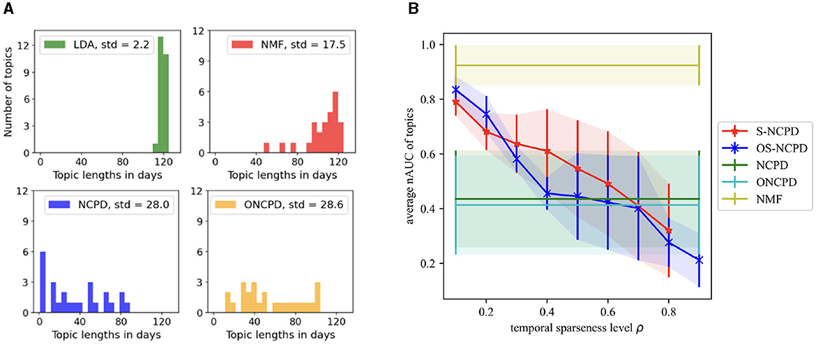
Figure 3. Topic length statistics for Headlines dataset for various methods. (A) Histograms of the α-effective lengths with α = 0.6 of all 25 topics learned by LDA, NMF, NCPD, and ONCPD. (B) Average nAUC scores (with one standard deviation shown as the shades) of topic lengths vs. temporal sparseness level ρ for S-NCPD, OS-NCPD, NCPD, ONCPD, and NMF. Tensor-based methods are able to learn mixed-length, overall shorter-lasting topics, while the sparseness-constrained methods allow for control of the desired topic length through the sparseness-level-parameter ρ. Smaller nAUC scores indicate shorter-lasting topics, see Section 2.2.
The upshot of our experiments are summarized below.
1. (Figure 3) LDA and NMF mostly learn long-lasting topics (average nAUC scores >0.9) with small variability in topic length (std < 0.15 nAUC)
2. (Figure 3B) NCPD and ONCPD learn mixed-scale, overall shorter-lasting topics (average nAUC scores 0.4-0.42) with larger variability (std>0.57 nAUC) than LDA and NMF.
3. (Figure 4) OS-NCPD is significantly more efficient in reducing the reconstruction error than S-NCPD.
4. (Figure 3B) S-NCPD and OS-NCPD learn topics of controlled lengths, where average nAUC scores tend to decay linearly (from 0.8-0.92 to 0.3-0.38) as one increases the sparseness level ρ; S-NCPD has larger variability of nAUC scores of the learned topics than OS-NCPD for when targetted to short- or long-lasting topics (ρ∈(0, 0.4)∪(0.8, 1)); For ρ∈(0.5, 0.7), both have large variability (std ≈0.4 nAUC). See also Figures 5, 6.
5. (Figures 7–9) OS-NCPD learns significantly more coherent topics (in terms of the Cv score) than S-NCPD.
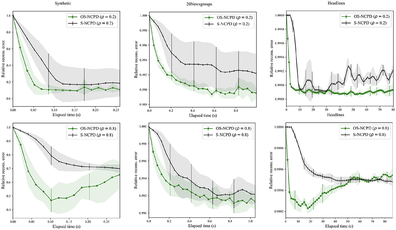
Figure 4. Plots of relative reconstruction error in the time of S-NCPD (black) and OS-NCPD (green) for three datasets: Synthetic tensor (left), 20 Newsgroups (middle), and News Headlines (right). Average and one standard deviation of relative reconstruction errors among ten trials with random initialization are shown.
Figure 5. Twenty five temporal topics are learned from ABC News Headlines dataset [a tensor of shape (Time × Words × Docs) = (203 × 7, 000 × 700)] via LDA. We show three top keywords for each topic and its time evolution as a heatmap, indexed by years. The heapmaps are normalized such that the sum of the weights over the whole topic at each time period equals one. “cv” refers to the Cv topic coherence score.
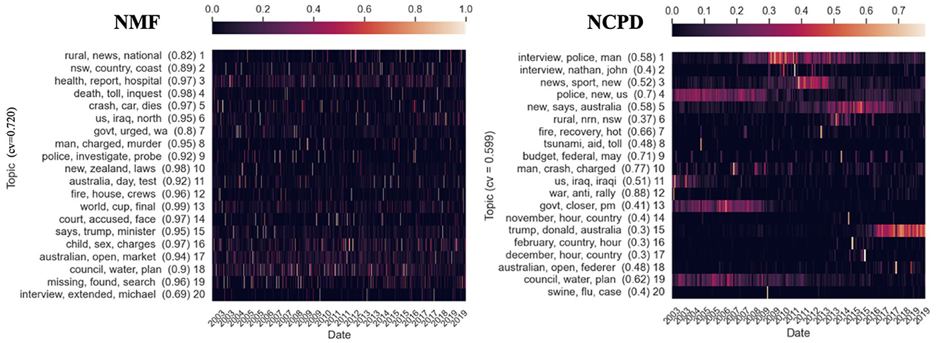
Figure 6. Twenty temporal topics are learned from ABC News Headlines dataset [a tensor of shape (Time × Words × Docs) = (203 × 7, 000 × 700)] via NMF and NCPD. The prevalence (measured by nAUC scores) of each topic is shown in parentheses. We show three top keywords for each topic and its time evolution as a heatmap, indexed by years. The heapmaps are normalized so that the rows sum to one. “cv” refers to the Cv topic coherence score.
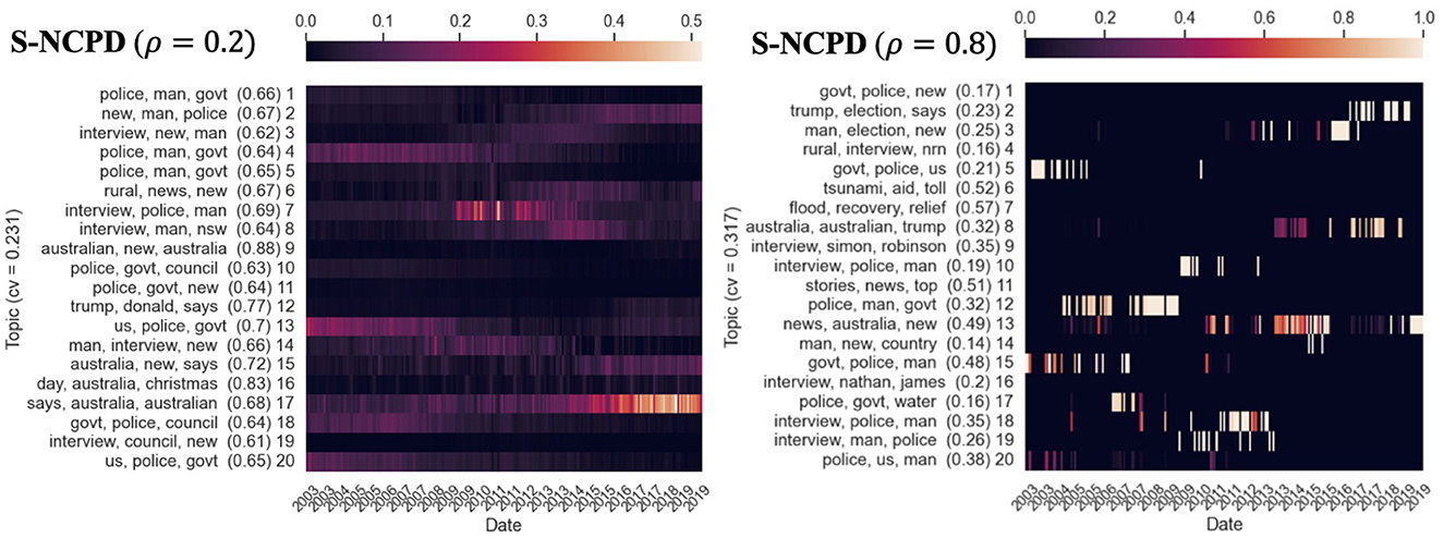
Figure 7. Twenty temporal topics are learned from ABC News Headlines dataset [a tensor of shape (Time × Words × Docs) = (203 × 7, 000 × 700)] via S-NCPD with various temporal sparseness levels ρ = 0.2 and 0.8. We show three top keywords for each topic and its time evolution as a heatmap, indexed by years. The prevalence (measured by nAUC scores) of each topic is shown in parentheses. The heapmaps are normalized so that the rows sum to one. “cv” refers to the Cv topic coherence score.
Figure 3A demonstrates the histograms of the lengths of all 25 topics in the Headlines dataset with α = 0.6. We can see that LDA produces very similar in length longer topics. Among LDA, NMF, NCPD, and ONCPD, only NCPD is able to pinpoint the six shortest topics with the effective length under 10 days for 60% of their content (compare with Figure 6). Then, ONCPD has the most length variability: sample standard deviations of the lengths of the topics discovered are 2.16, 17.54, 28.02, and 28.6 respectively for LDA, NMF, NCPD, and ONCPD methods.
Figure 3B plots the “length” of the learned topics measured as the average nAUC scores against the temporal sparseness level ρ. It is evident that NMF mostly learns long-lasting topics (average nAUC scores >0.9) with small variability in topic length (std < 0.15 nAUC). On the contrary, NCPD and OCNPD mixed-scale, overall shorter-lasting topics (average nAUC scores 0.4-0.42) with larger variability (std>0.57 nAUC) than NMF (see also Figures 6, 9). While one cannot control the temporal structure of topics to be learned via these methods, we see that the average topic lengths for S-NCPD and OS-NCPD decay linearly in the temporal sparseness level ρ. There, the average nAUC scores tend to decay linearly (from 0.8 to 0.2) as one increases the sparseness level ρ. As for the variability of nAUC scores (i.e., the range of temporal scales of the learned topics), S-NCPD has larger variability of nAUC scores of the learned topics than OS-NCPD for when targetted to short- or long-lasting topics (ρ∈(0, 0.4)∪(0.8, 1)); For ρ∈(0.5, 0.7), both have large variability (std ≈0.4 nAUC), resembling NCPD and ONPCD (see Figure 9 left). Furthermore, the topics learned by NCPD and OCNDP have similar and high Cv-scores (≈0.599 and ≈0.506, resp.) compared to NMF and LDA (≈0.720 and ≈0.468, resp.) (see Figures 5, 6, 9).
Figure 4 shows relative reconstruction error in time of S-NCPD and OS-NCPD with ρ∈{0.2, 0.8} for synthetic tensor of shape (100 × 200 × 300), the semi-synthetic 20 Newsgroups tensor (Section 4.2), and the News Headlines tensor. The average relative reconstruction errors are shown with one standard deviation in shades. In all experiments, we see that OS-NCPD decreases the objective value much faster than S-NCPD. Since we use a heuristic solver (Algorithm 1) for solving the sparsity-constrained nonnegative least squares, the objective value can fluctuate as the algorithms proceed. This is in contrast to the monotone decrease in the objective value for NCPD and ONCPD observed in Figure 2 [23].
Figure 6 shows the topics learned by NMF and NCPD and their Cv scores. NCPD topics have Cv score ≈0.599. Enforcing sparseness constraints would restrict the types of topics to be learned by the tensor factorization methods but is expected to hinder topic coherence due to the additional sparseness constraint that the optimization procedure must comply with. As expected, as in Figure 7, the topics learned by S-NCPD with ρ = 0.2 and ρ = 0.8 have Cv score ≈0.231 and ≈0.317, respectively. In Figure 8, topics learned by OS-NCPD with the same sparseness levels ρ have much higher Cv scores, namely ≈0.487 and ≈0.450 for ρ = 0.2 and ρ = 0.8, respectively. This shows that the online nature of OS-NCPD improves not only computational efficiency but also topic coherence. We observed the same phenomenon in many experiments with wide range of ρ values. It is worth to investigate further theoretical justification of this curious fact.
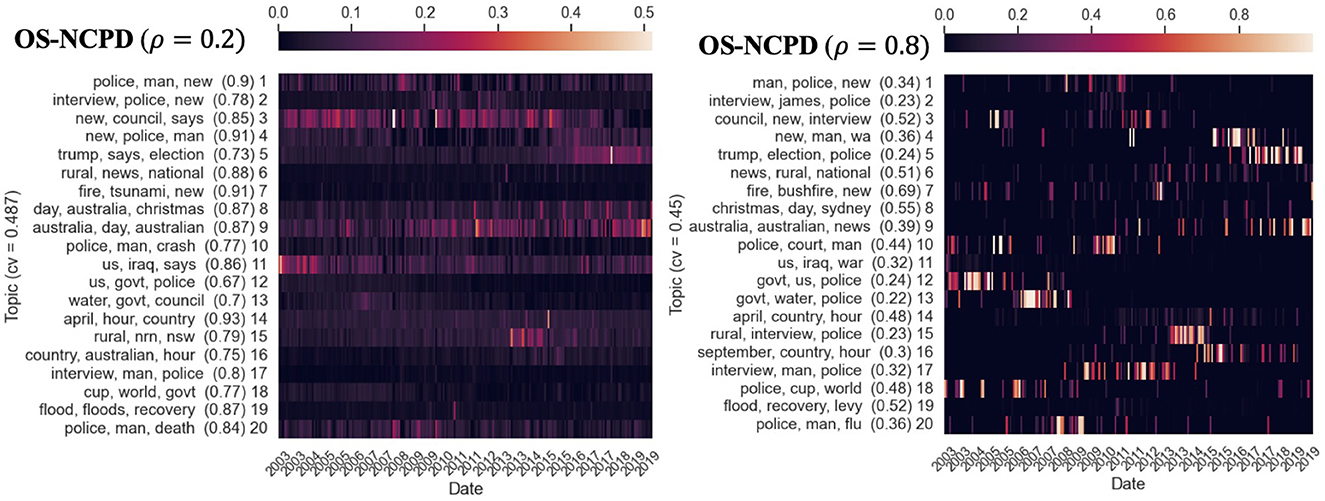
Figure 8. Twenty temporal topics are learned from ABC News Headlines dataset [a tensor of shape (Time × Words × Docs) = (203 × 7, 000 × 700)] via OS-NCPD with various temporal sparseness levels α. We show three top keywords for each topic and its time evolution as a heatmap, indexed by years. The prevalence (measured by nAUC scores) of each topic is shown in parentheses. The heapmaps are normalized so that the rows sum to one. “cv” refers to the Cv topic coherence score.
We give a more detailed discussion through Figures 5–9.

Figure 9. Twenty temporal topics are learned from ABC News Headlines dataset [a tensor of shape (Time × Words × Docs) = (203 × 7, 000 × 700)] via ONCPD and OS-NCPD (with ρ = 0.5). We show three top keywords for each topic and its time evolution as a heatmap, indexed by years. The prevalence (measured by nAUC scores) of each topic is shown in parentheses. The heapmaps are normalized so that the rows sum to one. “cv” refers to the Cv topic coherence score.
4.3.1 NMF and LDA: learn mostly long-lasting topics
In order to use NMF to detect topics and their time evolution, we may preprocess the 3D tensor into a Time×Words tensor in the following two ways: (1) unfold the 3D tensor so that the resulting 2D tensor is a concatenation of the word frequency vectors of individual documents (total of 700*203); (2) average the word frequency vectors for all 700 documents within each month into a single word frequency vector. Applying NMF on (1) does not seem to detect topics of clear temporal structure, as shown in Figure 6. The prevalence of the topics (measured by nAUC scores) shown in Figure 6 indicates that NMF can only learn long-lasting topics (of nAUC scores close to one).
Preprocessing (2) suffers from merging many documents of potentially distinct topics into one, so one can expect the topics detected by NMF would mix keywords from different topics. We omitted a similar plot for this experiment. Also, LDA was only able to detect topics whose prevalence spans the entire temporal horizon (see Figure 5). In comparison to the semi-synthetic data in Figure 2, we find that LDA is not effective in detecting short-lasting and periodic topics from real data.
4.3.2 NCPD and ONCPD: learn mixed-scale, overall shorter-lasting topics
We observe in Figure 6 that (standard) NCPD automatically detects short-lasting, periodic (e.g., topic 20 on “swine”, “flu”, and “case”), and long-lasting topics (e.g., topic 4 on “police”, “news”, and “us”). In particular, as seen in Figure 6, NCPD is able to learn topics with small nAUC scores (e.g., nAUC = 0.4 for topic 20) as well as large nAUC scores (e.g., nAUC = 0.88 for topic 12). From the keywords of these topics, we observe relatively more cohesive topics that align with real-world events. E.g., topic 18 (“Australian” “open”, “Federer”), topic 9 (“budget”, “federal”, “May”). The topics learned by ONCPD share very similar characteristics to the ones learned by NCPD (see Figure 9).
Compared to the NMF experiment in Figure 6, NCPD can detect meaningful topics with a clear temporal structure. The key difference is that NCPD processes the thrid-order tensor data at once, where multiple documents within the same temporal documents (specifically, 708 documents in our Headlines dataset) are considered to be simultaneous while keeping different documents separate so that no two documents of distinct topics are merged in the pre-processing stage [as in NMF pre-processing scheme (2)]. We mention that while it is possible to use the final reconstruction error of NCPD to assess the goodness of the overall factorization, computing the reconstruction error in this case is prohibitively expensive as it involves processing 20 tensors (one for each topic) of shape (203 × 7, 000 × 700).
4.3.3 S-NCPD and OS-NCPD: controlled temporal structure
While we see that NCPD can detect topics of various temporal characteristics, it would be beneficial to have methods for actively controlling the desired length of topics. We proposed S-NCPD and OS-NCPD for this purpose. If we use sparseness level α = 0.2 for S-NCPD as in Figure 7, it would restrict NCPD to learn topics whose time evolution (i.e., the corresponding columns in the time×topic factor C matrix) has sparseness level 0.2, so it is rather evenly distributed over the entire time horizon. On the other hand, using α = 0.8 as in Figure 7 now promotes learning only topics with much shorter prevalence. This additional temporal sparseness restriction in general results in fewer distinct topics compared to vanilla NCPD but could uncover new topics that were not detected by vanilla NCPD. For instance, with sparseness level 0.8 (Figure 7), we uncover a topic (topic 7: “flood”, “recovery”, “relief”) not readily discovered by vanilla NCPD with rank 20 by the top keywords. A similar discussion as above also applies to OS-NCPD (see Figure 8). However, there are notable differences in the standard deviation of the nAUC scores of the topics learned by S-NCPD and OS-NCPD. When ρ is tuned so that either short-lasting or long-lasting topics are targeted, OS-NCPD tends to result in a smaller variation of the nAUC scores than S-NCPD (see Figure 3B).
Another interesting observation is that OS-NCPD seems to give topics that are more coherent than the ones computed by S-NCPD (in terms of the Cv score) (Figure 8).
4.3.4 Computational efficiency of OS-NCPD over S-NCPD
An obvious disadvantage of S-NCPD is the computational cost of finding the sparsity-constrained nonnegative CP decomposition and the memory required to store the whole tensor. We show that OS-NCPD provides a viable alternative to the S-NCPD method for the limited computational resources.
We compare the performance of S-NCPD (4) and OS-NCPD (6) on three datasets (synthetic tensor, semi-synthetic 20 Newsgroup, and News Headlines) in terms of the relative reconstruction error at various temporal sparseness levels. For each dataset, we run each of the algorithms with rank 5 ten times with randomly initialized factor matrices with independent entries sampled uniformly from the interval [0, 1]. In Figure 4, the average of reconstruction errors [computed by (1)] with 1 standard deviation are shown by the solid lines and shaded regions of respective colors.
OS-NCPD works with smaller data tensors of size (words, batch′, time) (see also the discussion in Section 2.1.5), where we may take batch′ arbitrarily smaller than the actual number of documents batch in the original data tensor. From this, one can expect that the OS-NCPD is more computationally efficient than the OS-NCPD algorithm. Indeed, in Figure 4, we see that OS-NCPD is able to decrease the reconstruction error much more rapidly than the standard S-NCPD, although given enough time and computational budget, OS-NCPD may eventually end up with a smaller reconstruction error than OS-NCPD as in the 20 Newsgroups data in Figure 4.
Also, it is important to reiterate that such a computational gain in using OS-NCPD in dynamic topic modeling does not necessarily entail a compromise in the ability of NCPD to learn a variety of short-term and long-term topics (e.g., in the News Headlines).
5 Conclusion and future work
We demonstrate nonnegative CANDECOMP/PARAFAC decomposition (NCPD) as a powerful dynamic topic modeling technique capable of detecting short-lasting and periodic topics along with long-lasting topics in dynamic text datasets. In order to overcome the lack of controllability of topic lengths in NCPD, we proposed two new methods that can actively control the lengths of topics through an additional sparseness constraint. We propose both the offline (S-NCPD) and online (OS-NCPD) versions of such methods. We discuss and compare the temporal topic patterns learned through each of these methods. We propose different ways to measure the lengths of the discovered topics and validate the ability of tensor methods to discover short-term topics quantitatively. We observe that both S-NCPD and OS-NCPD extract fewer distinct, but potentially new topics depending on the temporal sparseness parameter, where the average topic lengths decrease linearly as we increase that parameter. For large datasets, OS-NCPD serves as a viable alternative for learning topics and their temporal patterns, retaining the ability to detect controlled short-lasting topics.
Among the natural future directions of the current work, is improving the efficiency of nonnegative tensor decompositions, e.g., by employing geometry-preserving tensor dimension reduction techniques (such as, [56]), running NCPD fitting algorithms on a compressed tensor, and subsequent recovery of the topics from their compressed representation. Additionally, it is interesting to study the prominence evolution of a particular topic with respect to the others via tensor extensions of the recently proposed GuidedNMF algorithm [57]. We also aim to study the relation between the sparseness level in the temporal component of the tensor and the rank of the decomposition.
Finally, the proposed methods S-NCPD and OS-NCPD are not specific for a particular type of data. Finding the topics, or clusters of data, with controlled localization properties would be important for various applications (not considered in this paper) where non-negative low-rank matrix and tensor methods are extensively employed, including the text data coming from multiple sources [58], image analysis [13, 59, 60], or computational biology [61–63].
Data availability statement
The datasets presented in this study can be found in online repositories. The names of the repository/repositories and accession number(s) can be found below: https://github.com/lara-kassab/dynamic-tensor-topic-modeling.
Author contributions
HL and JY developed the algorithm and code for S-NCPD and OS-NCPD. LK, AK, and DM designed dynamic topic modeling experiments. ER developed quantitative measures of topic lengths. All authors contributed equally to the paper writing.
Funding
The author(s) declare financial support was received for the research, authorship, and/or publication of this article. DM, DN, and ER were partially funded by NSF DMS 2011140. ER was also partially funded by NSF DMS 2309685 and NSF DMS 2108479. HL was partially funded by NSF DMS 2206296 and DMS 2010035.
Acknowledgments
We thank Jacob Moorman for his contributions to the code used. ER is also thankful to Maria Avdeeva for very useful discussions.
Conflict of interest
The authors declare that the research was conducted in the absence of any commercial or financial relationships that could be construed as a potential conflict of interest.
Publisher's note
All claims expressed in this article are solely those of the authors and do not necessarily represent those of their affiliated organizations, or those of the publisher, the editors and the reviewers. Any product that may be evaluated in this article, or claim that may be made by its manufacturer, is not guaranteed or endorsed by the publisher.
References
1. Blei DM, Lafferty JD. Dynamic topic models. In: Proceedings of the 23rd International Conference on Machine Learning. Pittsburg, PA: ACM (2006). p. 113–120. doi: 10.1145/1143844.1143859
2. Hu J, Sun X, Lo D, Li B. Modeling the evolution of development topics using dynamic topic models. In: 2015 IEEE 22nd International Conference on Software Analysis, Evolution, and Reengineering (SANER). Montreal, QC: IEEE (2015). p. 3-12.
3. Iwata T, Yamada T, Sakurai Y, Ueda N. Online multiscale dynamic topic models. In: Proceedings of the 16th ACM SIGKDD International Conference on Knowledge Discovery and Data Mining. Washington, DC: ACM (2010). p. 663–672.
4. Saha A, Sindhwani V. Learning evolving and emerging topics in social media: a dynamic NMF approach with temporal regularization. In: Proceedings of the fifth ACM International Conference on Web Search and Data Mining. Seattle, WA: ACM (2012). p. 693–702.
5. Wang C, Blei D, Heckerman D. Continuous time dynamic topic models. arXiv[preprint] arXiv:12063298. (2012). doi: 10.48550/arXiv.1206.3298
6. Greene D, Cross JP. Exploring the political agenda of the European parliament using a dynamic topic modeling approach. Polit Anal. (2017) 25:77–94. doi: 10.1017/pan.2016.7
7. Belford M, MacNamee B, Greene D. Ensemble topic modeling via matrix factorization. In: 24th Irish Conference on Artificial Intelligence and Cognitive Science (AICS'16), Dublin, Ireland, 20-21 September 2016. Dublin: CEUR Workshop Proceedings (2016).
8. Cichocki A, Zdunek R, Amari Si. Nonnegative matrix and tensor factorization [lecture notes]. IEEE Signal Process Mag. (2007) 25:142–5. doi: 10.1109/MSP.2008.4408452
9. Pathak AR, Pandey M, Rautaray S. Adaptive model for dynamic and temporal topic modeling from big data using deep learning architecture. In J Intellig Syst Appl. (2019) 11:13. doi: 10.5815/ijisa.2019.06.02
10. Rennie J. 20 Newsgroups. (2008). Available online at: http://qwone.com/~jason/20Newsgroups/ (accessed January 14, 2008).
11. Kulkarni R. A million news headlines. In: Harvard Dataverse. Cambridge, MA: Harvard Dataverse (2018).
13. Lee DD, Seung HS. Learning the parts of objects by non-negative matrix factorization. Nature. (1999) 401:788. doi: 10.1038/44565
14. Lee D, Seung HS. Algorithms for non-negative matrix factorization. In: Advances in neural information processing systems. Denver, CO: MIT Press (2000). 13p.
15. Hoffman M, Bach FR, Blei DM. Online learning for latent dirichlet allocation. In: Advances in Neural Information Processing Systems. Princeton: Citeseer (2010). p. 856–864.
16. Kolda TG, Bader BW. Tensor decompositions and applications. SIAM Rev. (2009) 51:455–500. doi: 10.1137/07070111X
17. Rabanser S, Shchur O, Günnemann S. Introduction to tensor decompositions and their applications in machine learning. arXiv [preprint]arXiv:171110781. (2017).
18. Xiong L, Chen X, Huang TK, Schneider J, Carbonell JG. Temporal collaborative filtering with bayesian probabilistic tensor factorization. In: Proceedings of the 2010 SIAM international conference on data mining. Philadelphia: SIAM (2010). p. 211–222.
19. Bahargam S, Papalexakis E. A constrained coupled matrix-tensor factorization for learning time-evolving and emerging topics. arXiv [preprint] arXiv:180700122. (2018). doi: 10.48550/arXiv.1807.00122
20. Bader BW, Berry MW, Browne M. Discussion tracking in Enron email using PARAFAC. In: Survey of Text Mining II. Cham: Springer (2008). p. 147–163.
21. Dunlavy DM, Kolda TG, Acar E. Temporal link prediction using matrix and tensor factorizations. ACM Trans Knowl Discov Data (TKDD). (2011) 5:1–27. doi: 10.1145/1921632.1921636
22. Ahn M, Eikmeier N, Haddock J, Kassab L, Kryshchenko A, Leonard K, et al. On large-scale dynamic topic modeling with nonnegative CP tensor decomposition. arXiv [preprint]arXiv:200100631. (2020). doi: 10.1007/978-3-030-79891-8_8
23. Lyu H, Strohmeier C, Needell D. Online nonnegative CP-dictionary learning for Markovian data. J Mach Learn Res. (2022) 23:1–50. doi: 10.48550/arXiv.2009.07612
24. Lu HM. Detecting short-term cyclical topic dynamics in the user-generated content and news. Decis Support Syst. (2015) 70:1–14. doi: 10.1016/j.dss.2014.11.006
25. Correia FA, Nunes JL, Alves PH, Lopes H. Dynamic topic modeling with tensor decomposition as a tool to explore the legal precedent relevance over time. In: Proceedings of the ACM Symposium on Document Engineering 2023. Limerick: ACM (2023). p. 1–10.
26. Zhao J, Zhang Y, Schlueter DJ, Wu P, Kerchberger VE, Rosenbloom ST, et al. Detecting time-evolving phenotypic topics via tensor factorization on electronic health records: Cardiovascular disease case study. J Biomed Inform. (2019) 98:103270. doi: 10.1016/j.jbi.2019.103270
27. Ahn M, Eikmeier N, Haddock J, Kassab L, Kryshchenko A, Leonard K, et al. On large-scale dynamic topic modeling with nonnegative CP tensor decomposition. In: Advances in Data Science. Cham: Springer (2021). p. 181–210.
28. Hoyer PO. Non-negative matrix factorization with sparseness constraints. J Mach Learn Res. (2004) 5:1457–69.
29. Lyu H. Stochastic regularized majorization-minimization with weakly convex and multi-convex surrogates. In: To appear in Journal of Machine Learning Research. (2023).
30. Chen H, Li J. Modeling relational drug-target-disease interactions via tensor factorization with multiple web sources. In: The World Wide Web Conference. San Francisco, CA: ACM (2019). p. 218-227.
31. Papalexakis E, Pelechrinis K, Faloutsos C. Spotting misbehaviors in location-based social networks using tensors. In: Proceedings of the 23rd International Conference on World Wide Web. Seoul: ACM (2014). p. 551–552.
32. Balasubramaniam T, Nayak R, Luong K, Bashar MA. Identifying Covid-19 misinformation tweets and learning their spatio-temporal topic dynamics using Nonnegative Coupled Matrix Tensor Factorization. Soc Netw Analy Mining. (2021) 11:57. doi: 10.1007/s13278-021-00767-7
33. Balasubramaniam T, Nayak R, Bashar MA. Understanding the spatio-temporal topic dynamics of covid-19 using nonnegative tensor factorization: a case study. In: 2020 IEEE symposium series on computational intelligence (SSCI). Canberra, ACT: IEEE (2020). p. 1218–1225.
34. Yu S, Zhou Z, Chen B, Cao L. Generalized temporal similarity-based nonnegative tensor decomposition for modeling transition matrix of dynamic collaborative filtering. Inf Sci. (2023) 632:340–57. doi: 10.1016/j.ins.2023.03.018
35. Heiler M, Schnörr C, Bennett KP, Parrado-Hernández E. Learning sparse representations by non-negative matrix factorization and sequential cone programming. J Mach Learn Res. (2006) 7:1385–407.
36. Tuy H. Convex programs with an additional reverse convex constraint. J Optim Theory Appl. (1987) 52:463–86. doi: 10.1007/BF00938217
37. Heiler M, Schnorr C. Learning non-negative sparse image codes by convex programming. In: Tenth IEEE International Conference on Computer Vision (ICCV'05) Volume 1. Beijing: IEEE (2005). p. 1667–1674.
38. Lyu H, Li Y. Block majorization-minimization with diminishing radius for constrained nonconvex optimization. arXiv [preprint]arXiv:201203503. (2023). doi: 10.48550/arXiv.2012.03503
39. Carroll JD, Chang JJ. Analysis of individual differences in multidimensional scaling via an N-way generalization of “eckart-young” decomposition. Psychometrika. (1970) 35:283–319. doi: 10.1007/BF02310791
40. Harshman RA. Foundations of the PARAFAC procedure: models and conditions for an “explanatory” multimodal factor analysis. In: UCLA Working Papers in Phonetics. Ann Arbor: University Microfilms (1970). p. 1–84.
41. Buciu I. Non-negative matrix factorization, a new tool for feature extraction: theory and applications. Int J CompCommun Control. (2008) 3:67–74.
42. Kuang D, Choo J, Park H. Nonnegative matrix factorization for Interactive Topic Modeling and Document Clustering. In: Partitional Clustering Algorithms. Cham: Springer (2015). p. 215-243.
43. Bertsekas DP. Nonlinear programming. In: Athena scientific Belmont. Athena Scientific Belmont (1999).
44. Wright SJ. Coordinate descent algorithms. Mathem Prog. (2015) 151:3–34. doi: 10.1007/s10107-015-0892-3
45. Shashua A, Hazan T. Non-negative tensor factorization with applications to statistics and computer vision. In: Proceedings of the 22nd International Conference on Machine Learning. Bonn: ACM (2005). p. 792–799.
46. Heiler M, Schnörr C. Controlling sparseness in non-negative tensor factorization. In: Computer Vision-ECCV 2006:9th European Conference on Computer Vision, Graz, Austria, May 7-13, 2006. Graz: Springer (2006). p. 56–67.
47. Lobo MS, Vandenberghe L, Boyd S, Lebret H. Applications of second-order cone programming. Linear Algebra Appl. (1998) 284:193–228. doi: 10.1016/S0024-3795(98)10032-0
48. Alizadeh F, Goldfarb D. Second-order cone programming. Mathem Prog. (2003) 95:3–51. doi: 10.1007/s10107-002-0339-5
49. Beck A, Tetruashvili L. On the convergence of block coordinate descent type methods. SIAM J Optimizat. (2013) 23:2037–60. doi: 10.1137/120887679
50. Pedregosa F, Varoquaux G, Gramfort A, Michel V, Thirion B, Grisel O, et al. Scikit-learn: machine learning in Python. J Mach Learn Res. (2011) 12:2825–30.
51. Boutsidis C, Gallopoulos E, SVD. based initialization: a head start for nonnegative matrix factorization. Pattern Recognit. (2008) 41:1350–62. doi: 10.1016/j.patcog.2007.09.010
52. Kossaifi J, Panagakis Y, Anandkumar A, Pantic M. TensorLy: tensor learning in Python. J Mach Learn Res. (2019) 20:1–6.
53. Řehůřek R, Sojka P. Software framework for topic modelling with large Corpora. In: Proceedings of the LREC 2010 Workshop on New Challenges for NLP Frameworks. Valletta, Malta: ELRA (2010). p. 45–50. Available online at: http://is.muni.cz/publication/884893/en
54. Röder M, Both A, Hinneburg A. Exploring the space of topic coherence measures. In: Proceedings of the eighth ACM International Conference on Web Search and Data Mining. Shanghai: ACM (2015). p. 399–408.
55. Bird S, Klein E, Loper E. Natural Language Processing with Python: Analyzing Text with the Natural Language Toolkit. Sebastopol, CA: O'Reilly Media, Inc. (2009).
56. Iwen MA, Needell D, Rebrova E, Zare A. Lower memory oblivious (tensor) subspace embeddings with fewer random bits: modewise methods for least squares. SIAM J Matrix Anal Appl. (2021) 42:376–416. doi: 10.1137/19M1308116
57. Vendrow J, Haddock J, Rebrova E, Needell D. On a guided nonnegative matrix factorization. In: ICASSP 2021-2021 IEEE International Conference on Acoustics, Speech and Signal Processing (ICASSP). Toronto, ON: IEEE (2021). p. 3265–32369.
58. Vendrow J, Haddock J, Needell D. A generalized hierarchical nonnegative tensor decomposition. In: ICASSP 2022-2022 IEEE International Conference on Acoustics, Speech and Signal Processing (ICASSP). Singapore: IEEE (2022). p. 4473–4477.
59. Kumar N, Uppala P, Duddu K, Sreedhar H, Varma V, Guzman G, et al. Hyperspectral tissue image segmentation using semi-supervised NMF and hierarchical clustering. IEEE Trans Med Imaging. (2018) 38:1304–13. doi: 10.1109/TMI.2018.2883301
60. He Y, Lu H, Xie S. Semi-supervised non-negative matrix factorization for image clustering with graph Laplacian. Multimed Tools Appl. (2014) 72:1441–63. doi: 10.1007/s11042-013-1465-1
61. Brunet JP, Tamayo P, Golub TR, Mesirov JP. Metagenes and molecular pattern discovery using matrix factorization. Proc Nat Acad Sci. (2004) 101:4164–9. doi: 10.1073/pnas.0308531101
62. Kim H, Park H. Sparse non-negative matrix factorizations via alternating non-negativity-constrained least squares for microarray data analysis. Bioinformatics. (2007) 23:1495–502. doi: 10.1093/bioinformatics/btm134
Keywords: topic modeling, temporal data, sparseness, nonnegative CP decomposition, online tensor factorization
Citation: Kassab L, Kryshchenko A, Lyu H, Molitor D, Needell D, Rebrova E and Yuan J (2024) Sparseness-constrained nonnegative tensor factorization for detecting topics at different time scales. Front. Appl. Math. Stat. 10:1287074. doi: 10.3389/fams.2024.1287074
Received: 01 September 2023; Accepted: 10 June 2024;
Published: 22 July 2024.
Edited by:
Abiy Tasissa, Tufts University, United StatesReviewed by:
Soraya Ezazipour, Oklahoma State University Oklahoma City, United StatesJuntao You, Shenzhen University, China
Copyright © 2024 Kassab, Kryshchenko, Lyu, Molitor, Needell, Rebrova and Yuan. This is an open-access article distributed under the terms of the Creative Commons Attribution License (CC BY). The use, distribution or reproduction in other forums is permitted, provided the original author(s) and the copyright owner(s) are credited and that the original publication in this journal is cited, in accordance with accepted academic practice. No use, distribution or reproduction is permitted which does not comply with these terms.
*Correspondence: Hanbaek Lyu, hlyu@math.wisc.edu