Subnetwork inclusion and switching of multilevel Boolean networks preserve parameter graph structure and dynamics

This study addresses a problem of correspondence between dynamics of a parameterized system and the structure of interactions within that system. The structure of interactions is captured by a signed network. A network dynamics is parameterized by collections of multi-level monotone Boolean functions (MBFs), which are organized in a parameter graph PG. Each collection generates dynamics which are captured in a structure of recurrent sets called a Morse graph. We study two operations on signed graphs, switching and subnetwork inclusion, and show that these induce dynamics-preserving maps between parameter graphs. We show that duality, a standard operation on MBFs, and switching are dynamically related: If M is the switch of N, then duality gives an isomorphism between PG(N) and PG(M) which preserves dynamics and thus Morse graphs. We then show that for each subnetwork M ⊂ N, there are embeddings of the parameter graph PG(M) into PG(N) that preserve the Morse graph. Since our combinatorial description of network dynamics is closely related to switching ODE network models, our results suggest similar results for parameterized sets of smooth ODE network models of the network dynamics.

1 Introduction

The concept of a network plays a central role in systems biology, where it encodes interactions between the molecular species. Each directed edge has a sign, which represents either a monotonically increasing or monotonically decreasing effect of the source on the target. The restriction to monotone interactions suggests a possibility that there is a relationship between structure of the network and its emergent dynamics.

There are different types of dynamics that can be associated to a network. Some, like those generated by Boolean functions wherein each node can take on a value of 0 or 1, are very tightly linked to the structure of the network. On the other hand, the dynamics generated by ordinary differential equations (ODE) models with an interaction structure given by the network strongly depends on choice of non-linearities and parameters. Within the class of ODE network models, the question of limitations on dynamics imposed by network structure is much more difficult. In particular, one has to carefully define what constitutes the “same” dynamics to compare the dynamics of different networks. Traditional definitions used in comparison of dynamical systems include the concept of conjugate dynamics, or conjugate dynamics on a recurrent set Ω [1]. While the first condition is stronger, both conditions are very difficult to verify. To illustrate the difficulties, it is known that the hope that for a generic set of Morse-Smale systems the set Ω is finite is false [2].

In this study, we address the question of the relationship between network structure and its dynamics in the context of multi-valued Boolean systems in which each vertex can take on a set of integer values based on its number of out-edges. The approach is based on [3–6] Dynamic Signatures Generated by Regulatory Networks (DSGRN) which parameterizes the dynamics of a network with a collection of monotone Boolean functions (MBFs) that are compatible with its structure, that is, the monotonicity is compatible with the signs of the network edges. These collections are organized in a finite parameter graph PG that takes the form of a product graph PG = ∏_{u ∈ V}PG(u) where the product is over vertices of the network. Each node in PG represents a collection of MBFs called a DSGRN parameter or just parameter. The edges in PG represent adjacency within the collections of MBFs.

There is a correspondence [7] between each DSGRN parameter and the dynamics of a switching ODE system [8–16], whose dynamics can be captured by a finite state transition graph (STG). A switching ODE can be approximated arbitrarily well by a smooth ODE system; there are rigorous results [17–19] that connect smooth ODE dynamics to that of a switching system and thus STG. DSGRN uses a more compact description of the dynamics of an STG in the form of a Morse graph (MG). Nodes of a Morse graph are strongly connected components of the STG, and the edges of MG are given by reachability within the STG. Therefore, our description of the dynamics of network N consists of its parameter graph PG(N) with an associated collection of Morse graphs MG(N), one for each node. Since the parameter graph PG(N) provides direct correspondence between the collection of monotone Boolean functions and the continuous time ODE dynamics of smooth approximations of switching systems, comparing the PGs across networks provides a global comparison between dynamic repertoires of these networks for both discrete and continuous time dynamics.

The connection between parameterization of continuous dynamics of switching systems and collections of multi-valued Boolean models of the same network was also described in Abou-Jaoudé and Monteiro [20]. While DSGRN starts with switching ODE system and arrives at Boolean description of ODE parameter domains, Abou-Jaoudé and Monteiro [20] starts with collection of multi-valued Boolean models and uses switching system parameters to generate sequences of Boolean systems. Changes in the structure of attractors are examined as an analog of bifurcations. The parameter graph PG is equivalent to the collection of all monotone multi-valued Boolean systems compatible with network N in Abou-Jaoudé and Monteiro [20]. The set of attractors is represented as the set of leaves in the Morse graph, and therefore, our description of dynamics using Morse graphs is more general.

With a finite characterization of network dynamics, it is natural to ask whether homomorphisms of signed directed graphs preserve network dynamics D(N): = (PG(N),MG(N)). We emphasize that we seek maps that preserve the graph structure of PG(N), where the map preserves the relationships between nodes given by edges. Under such a map not only dynamics at individual parameters p is preserved, but also the changes in the dynamics (bifurcations) between neighboring parameters p, q ∈ PG(N) are preserved. While we do not answer this question in its full generality, we study two important homomorphisms. First is the so-called switch map, introduced in Zaslavsky [21], on signed directed graphs that switches the signs of all edges incident to a set of vertices. In an ODE model, a switch can be realized via a change of variables x → −x for all variables corresponding to this set of vertices and has been used for monotone systems and monotone cyclic feedback systems to bring them to a normal form [22–24]. Clearly, a switch map preserves incidence of all edges and also the number and sign of all closed loops [21, 25–27]. In Aracena et al. [26], it was shown that a switch preserves the maximum number of fixed points of a network across all strict Boolean systems for that network. Here, we show that the maximum number of fixed points is preserved due to the preservation of all dynamics: A switch map induces an involution on the parameter graph PG that preserves the STG and hence MG. This shows that the dynamics of the two networks is the same.

The second homomorphism we study is inclusion of a network as subgraph in another network. This is a very important example in systems biology where gene regulatory networks cannot be assumed to be in their final form as new experimental evidence may reveal additional genes (nodes) and edges. Since the basis of any scientific approach is to study small problems first before using that knowledge to tackle larger problems, we must understand if, and how, the dynamics D(M) of a subnetwork M persists within the dynamics D(N) of a larger network N. Within the DSGRN framework, at some parameters p ∈ PG, a particular edge can be constitutively ON or constitutively OFF. We show that at parameters p ∈ PG where all edges in N\M are either constitutively ON or constitutively OFF, the parameter graph PG(M) is a subgraph of PG(N). In fact, we describe precisely the conditions under which there are several isomorphic copies of the parameter graph PG(M) within PG(N), where each copy carries the same collection of dynamics MG(M).

The second homomorphism is strongly motivated by systems biology. Gene regulatory networks do not exist in isolation and interact with other networks. It is important to understand if and under what conditions the dynamics of subnetworks persist within a larger network. As a motivating example, consider [28] where they considered the interaction of the yeast cell cycle network with the pheromone-sensing network that stops the cell cycle in the presence of mating pheromone. The study concludes that in the absence of pheromone the cell cycle network drives parts of the pheromone network, while in the presence of pheromone the cell cycle is driven to a rest state. One can conceptualize this interaction by assuming that the cell cycle network on its own supports a periodic orbit corresponding to the cell cycle and the pheromone-sensing network supports a steady state. This study shows that both of these dynamical behaviors occur in the larger network comprised of both subnetworks but at different parameters. This insight leads to the conjecture that by changing parameters it is possible for one or the other behavior to prevail within the larger network; however, at intermediate parameters, completely new dynamics may emerge.

A further motivating example comes from examining the subnetworks of the cell cycle itself, which support multiple phenotypes. The dual view of the cell cycle as either a biochemical “clock” vs. a set of “dominos”, that is, a series of switches where the completion of one step is required for the completion of the next step, has been discussed for at least 35 years [29, 30]. Support for the biochemical clock view comes, among others, from studies that showed that even in the absence of cyclins, a cell cycle-associated program of periodic transcription program is intact [31]. On the other hand, a bistable switch facilitates transition from G1 to S phase of the cell cycle [5, 32, 33], and other switches likely facilitate other checkpoints. Since recent modeling work suggests that different cell cycle phenotypes are the result of changes in parameters [34], these two views can be reconciled by realizing that cell cycle network [31, 34] contains multiple positive and negative feedback loops. Since negative loops in isolation can support periodic behavior [35], while positive loops can support bistability [36], the cell cycle phenotype depends on particular parameters (i.e., cellular conditions) that determine which behavior dominates. For instance, in many cancers, the uncontrolled proliferation is caused by defective checkpoints [37, 38]. How the checkpoint steady state dynamics driven by positive loops interacts with periodic behavior driven by negative loops, and the proximity of these behaviors in the parameter space, may suggest perturbations that restore the checkpoint function.

Apart from addressing a general question of comparison of dynamic repertoires of networks, the work presented here provides the capability to answer the rigorously central hypothesis of motif theory [39–41] within systems biology. Motifs are small networks with 3-4 nodes each that are postulated to have a particular cellular function based on their dynamics. However, it is not clear whether independent motif dynamics persists after embedding into a larger network. Our work suggests conditions under which the independent motif dynamics can be observed within the larger network.

We illustrate our work on a small network N in Figure 1A throughout the study. There are two motifs embedded in this network: a mutual activation loop PL (positive loop) between z and y and a negative feedback loop NL x ⊣ y → z → x. Theorems 5.4, 5.5 describe how the dynamics of these loops persists within the larger network in Figure 1A. We outline these results here on network N, while leaving the details for the text that follows.

Figure 1

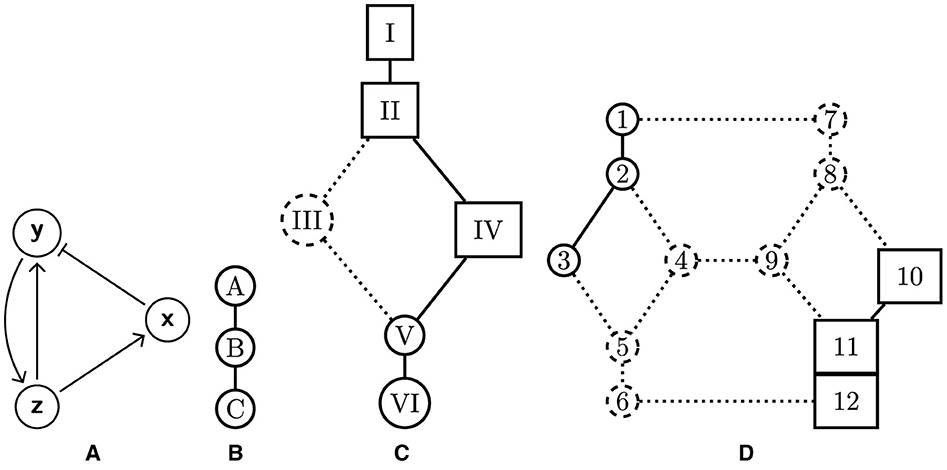
Figure 1. (A) Network N with positive loop motif PL between z and y and a negative loop motif NL x ⊣ y → z → x. (B) There are three monotone Boolean functions (MBF) at node x forming parameter factor graph PG(x); (C) six MBF forming PG(y); (D) twelve MBFs forming PG(z). The set of all parameters is PG(N) =PG(x) × PG(y) × PG(z). There are two embeddings of PG(NL) into PG(N). Both embeddings are products of PG(x) with subgraph of PG(y) and a subgraph of PG(z). When edge e:z → y is always ON, these subgraphs are {I,II, IV} and {10,11,12}, marked by square nodes. If the edge e:z → y is always OFF, the subgraphs are {IV,V, VI} and {1,2,3}, marked by circle nodes.

We represent all possible ways in which the network can function by enumerating a collection of monotone Boolean functions (MBF) (Section 2.1). These describe how the concentration levels of the input edge(s) of each node activate the output edges. Node x has single input and single output and there are three MBFs (see Table 1) that describe potential activation patterns of the output edge x ⊣ y in response to a Boolean input Z ∈ {0, 1}: a constant function with value 0 (A), a constant function with value 1 (C), and an identity function B. Figure 1B shows the structure of this set of MBFs where we join by an edge any MBFs that differ in a single value. This is the parameter factor graph PG(x).

Table 1

Table 1. Three monotone Boolean functions in PG(x) with Boolean input Z.

In Figure 1C shows PG(y) consisting of MBFs with two inputs and one output and in Figure 1D is PG(z) of MBFs with one input and two outputs. Their structure is explained in Tables 2, 3 later in the study. The parameter graph of the network N is PG(N) =PG(x) × PG(y) × PG(z), the product of the parameter factor graphs.

Table 2

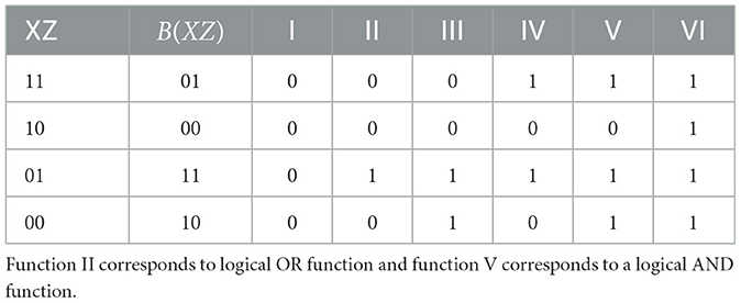
Table 2. Six monotone Boolean functions in PG(y) with Boolean inputs X and Z.

Table 3

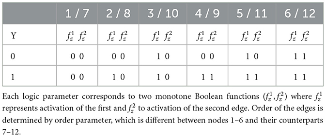
Table 3. Logic parameters of PG(z) corresponding to nodes 1-12 (first row).

As a consequence of Theorem 5.5, there are two subgraphs of PG(N) that are isomorphic to parameter graph of the negative loop PG(NL). These are products of PG(x) with subgraphs of PG(y) and PG(z) described in Figure 1. As explained in detail in Appendix B, there are four such embeddings of the parameter graph of the positive loop PG(PL) into PG(N) and consequently, at those parameters the dynamics of N is the same as that of the positive loop. These results make it possible to investigate relative positions of parameters that support bistability and those that support oscillations.

The organization of the study is as follows. In Section 2, we review the basic concepts of DSGRN: the parameter graph, state transition graph and Morse graph. In Section 3, we describe homomorphisms of signed graphs and a particular example of switching homomorphism. In Section 4, we show that the switching homomorphism preserves dynamics by inducing a graph isomorphism of the parameter graph that preserves dynamics. In Section 5, we start focusing on the network embedding as our second example of signed graph homomorphism. We formulate our main results as Theorem 5.4 about correspondence of dynamics at input inessential parameters and Theorem 5.5 at output inessential parameters. These Theorems are then proved in Sections 6 and 7, respectively. Section 8 contains discussion, while some proofs of the more technical results are delegated to the Section 8 and a detailed analysis of network N from Figure 1 is in Section 9.

2 Regulatory networks

A regulatory network N = (V, E, δ) is a directed graph with nodes V, directed edges E, and an edge sign function δ:E → {−1, 1}. We denote an edge from node u to node v without indicating its sign by u ⊸ v. The edge u ⊸ v is activating if ${\delta }_u^v=1$ and repressing if ${\delta }_u^v=-1$. Graphically, an activating edge is denoted by u → v and a repressing edge by u ⊣ v. The sources and targets of a node u are given by

$\begin{array}{c}\text{S}(u):=\left\{w\in V|w⊸u\in E\right\}\text{T}(u):=\left\{v\in V|u⊸v\in E\right\},\end{array}$

respectively.

2.1 Parameters

The parameterization of the dynamics of a network depends on the choice of model. We discuss two different types of models and briefly review literature on how the parameterizations of these two types of models are related. Boolean models compatible with regulatory network N have a long history [11, 42, 43], and their study remains an active research area [20, 44–46]. There are two closely related but distinct types of Boolean models. The standard Boolean network model considers a single Boolean function $f_u:{𝔹}^{\left|\text{S}(u)\right|}\to 𝔹$ at each node u which is monotone in each input respecting the edge sign δ. When a node is activated via f_u = 1, then this activated state, in turn, activates all edges from u to T(u) [44, 47–49]. The parameterization of such a network involves enumerating monotone Boolean functions f_u compatible with edge signs between S(u) and u. Often one is interested in non-degenerate [50] or, equivalently, observable [45] functions which are non-constant and each input affects the value of f_u.

An alternative and richer set of models starts with the original work of Thomas et al. [42]. They consider discrete dynamics where u can selectively activate some nodes in T(u), but not others, as this activation happens at different thresholds for different targets. This naturally leads to the consideration of multi-level Boolean functions, where the discrete levels of node u are related to the number of nodes in T(u). Parameterization of all such possible multi-valued Boolean functions compatible with the network structure has been described by Abou-Jaoudé and Monteiro [20] and by Cummins et al. [3, 4], and Gedeon [6], arriving at the same concept from different perspectives. The goal of Abou-Jaoudé and Monteiro [20] is to construct natural families of multi-valued Boolean functions that describe changes in the dynamics as a function of a continuous parameter. In order to do this, they need to relate the collection of multi-valued Boolean functions to a continuous time differential equation switching model where the change of continuous parameter then induces a sequence of multi-valued Boolean functions. The sequence of attractors of these functions constitutes a logical bifurcation diagram.

As mentioned in the introduction, our work [3] starts with an ODE switching model and realizes that the continuous parameter space of these models decomposes to a set of domains each of which admits the same dynamics, as described by a discrete state transition graph. This naturally leads to the representation of this decomposition in a form of a graph, called a parameter graph where each node represents one such domain and edges represent co-dimension one boundaries (immediate proximity) in the parameter space. As we describe in more detail below, each node of the parameter graph is specified by two sets of information: the ordering of thresholds of edges u to T(u), which we call below an order parameter, and the description of values of the multi-valued Boolean function f_u as a collection of monotone Boolean functions, each describing which Boolean inputs b ∈ 𝔹^S(u) activate a particular node v ∈ T(u). This collection is called below a logic parameter. This description is equivalent to the multi-valued Boolean function description of Abou-Jaoudé and Monteiro [20] (Definition 2).

We now start with rigorous description of the set of parameters associated with a regulatory network N = (V, E, δ). This set depends on the nodes V and the edges E but not on the sign of edges δ. For simplicity, we fix the network N and suppress these dependencies. We will reintroduce the dependencies in later sections as needed.

Let m_u: = |T(u)| denotes the number of target nodes of u. A u-order parameter is a bijection θ_u:T(u) → {1, …, m_u} which defines an ordering of the out-edges of u. The set of u-order parameters is denoted by Θ(u). A collection θ: = (_{θu)u ∈ V} is an order parameter. The set of all order parameters is given by Θ: = ∏_{u ∈ V} Θ (u). The target nodes are ordered based on how easy are they to activate: As level of expression of node u increases, the target nodes will activate in the order given by the value of the order parameter.

Let 𝔹: = ({0, 1};0 ≺ 1}) be a Boolean lattice with natural order 0 ≺ 1 and let 𝔹ⁿ be a lattice of Boolean n vectors with order induced component-wise by ≺.

To define the logic parameter, we need the following definition.

Definition 2.1. A function f : 𝔹ⁿ → 𝔹 is a positive monotone Boolean function if b¹ ≺ b² implies f(b¹) ≼ f(b²).

A u-logic parameter is a collection of positive monotone Boolean functions

$f_u=(f_u^1,\dots ,f_u^{m_u})$

satisfying the ordering condition

$\begin{array}{cc}{f}_u^1(b)\succcurlyeq \cdots \succcurlyeq f_u^{m_u}(b)& (1)\end{array}$

for all b ∈ 𝔹^S(u). The purpose of the function $f_u^{{\theta }_u(v)}$ is to describe when a given input b is above the activation threshold for the edge θ_u(v), that is, if $f_u^{{\theta }_u(v)}(b)=1$ then b is above the activation threshold for the edge u ⊸ v and if $f_u^{{\theta }_u(v)}(b)=0$ then b is below the activation threshold for the edge u ⊸ v. A collection f: = (_{fu)u ∈ V} is a logic parameter. The set of all u-logic parameters is denoted $\mathcal{L}(u)$, while the set of all logic parameters is $\mathcal{L}:={\prod }_{u\in V}\mathcal{L}(u)$.

The set of parameters is the product of logic and order parameters $\mathcal{P}:=\mathcal{L}\times \Theta$. We call $\mathcal{P}(u):=\mathcal{L}(u)\times \Theta (u)$ the set of u-parameters and note the parameters are given by the product $\mathcal{P}={\prod }_{u\in V}\mathcal{P}(u)$. The following section endows the set $\mathcal{P}$ with structure of a graph by defining adjacency between elements of $\mathcal{P}$.

In Section 2.3, we show that the u-logic parameter f_u can be equivalently described by a single multi-valued Boolean function g_u. Such a description is used in Abou-Jaoudé and Monteiro [20].

2.2 The parameter graph

Two u-parameter nodes, $(f_u,{\theta }_u),(g_u,{\varphi }_u)\in \mathcal{P}(u)$ are adjacent if exactly one of the following conditions is satisfied.

• Order adjacency: f_u = g_u and the values of the order parameters θ_u and ϕ_u are exchanged on a single pair of neighboring entries on which the logic parameters agree. Explicitly, there is an adjacent transposition π of {1, …, m_u} such that θ_u = π°ϕ_u and $f_u^i=g_u^{\pi (i)}$ for each i. Letting j be the index with j + 1 = π(j), we note that $f_u^j=g_u^{\pi (j)}$ and f_u = g_u together imply $f_u^j=f_u^{j+1}$.

• Logical adjacency: θ_u = ϕ_u and the u-logic parameters f_u and g_u differ in a single input. Explicitly, there is unique i ∈ {1, …, m_u} and unique b⁰ ∈ 𝔹^S(u) such that $f_u^i(b^0)\ne g_u^i(b^0)$. For j ≠ i, we require $f_u^j(b)=g_u^j(b)$ for all b ∈ 𝔹ⁿ and for b ≠ b⁰ we require $f_u^i(b)=g_u^i(b)$.

The u-factor graph is the undirected graph $\text{PG}(u):=(\mathcal{P}(u),\mathcal{E}(u))$ whose nodes are u-parameter nodes and whose edges are given by adjacency. The parameter graph $\text{PG}:=(\mathcal{P},\mathcal{E})$ is the Cartesian product PG: = ∏_{u ∈ V}PG(u). That is, there is an edge $(p^1,p^2)\in \mathcal{E}$ if and only if there is a unique u ∈ V such that $(p_u^1,p_u^2)\in \mathcal{E}(u)$ and $p_v^1=p_v^2$ for all v ≠ u.

We illustrate the parameter graph construction on network N in Figure 1A by constructing parameter factor graphs PG(y) in Figure 1C and PG(z) in Figure 1D.

First consider node y with S(y) = {x, z} and T(y) = {z}. Therefore, logic parameters are all monotone Boolean functions $f_y:{𝔹}^2\to 𝔹$ and since |T(y)| = 1 there is a single order parameter θ_z with value θ_y(z) = 1.

We list all MBFs at node y in Table 2. Note that the fact that the input from x is repressing is modeled by function B (see Equation 2) whose values are in the second column of the table. The edges in PG(y) in Figure 1C reflect parameter node adjacency.

Each node in the factor parameter graph PG(z) is a pair (f_z, θ_z) where f_z is a logic parameter and θ_z is an order parameter. Since there are two targets of z and T(z) = {x, y} there are two order parameters ${\theta }_z^1$ mapping x → 1 and y → 2, and ${\theta }_z^2$ mapping x → 2 and y → 1. Therefore, the logic parameter $f_z=(f_z^1,f_z^2)$ consists two MBFs, where $f_z^1$ models activation of the first target and $f_z^2$ the second target, given by the value of the order parameter. The order parameter ${\theta }_z^1$ corresponds to left half of PG(z) (nodes 1-6) and the order parameter ${\theta }_z^2$ to right half of PG(z) (nodes 7–12). Within each half, the order parameter is fixed, but the logic parameter changes and is described in Table 3.

2.3 Dynamics

The multi-valued Boolean dynamics associated with a network N = (V, E, δ) depends on a choice of parameter $p\in \mathcal{P}$ and the edge sign function δ.

The dynamics occurs on the state space

$X:={\displaystyle \prod _{u\in V}}{X}_u,X_u:=\left\{0,1,\dots ,m_u\right\}.$

We call x ∈ X a state of the network N. The multi-valued Boolean function at each node will update the state based on the input that depends on the state, order parameter θ and the edge sign function δ. The state x = (_{xu)u ∈ V} is mapped to an input to a node v via the input map

$B^v:X\to {𝔹}^{\text{S}(v)},B^v:={(B_u^v)}_{u\in \text{S}(v)}$

where

$\begin{array}{cc}{B}_u^v(x):=\{\begin{array}{ll}0,& \text{ if }{x}_u<{\theta }_u(v)\text{ and }{\delta }_u^v=1\text{ or }{x}_u\ge {\theta }_u(v)\text{ and }{\delta }_u^v=-1\\ 1,& \text{ if }{x}_u\ge {\theta }_u(v)\text{ and }{\delta }_u^v=1\text{ or }{x}_u<{\theta }_u(v)\text{ and }{\delta }_u^v=-1\end{array}.& (2)\end{array}$

Note that for activating edge u → v, if x_u is below (above) the activating threshold θ_u(v), then the input is 0 (1). This assignment is reversed if the edge is repressing.

An equivalent description of the u-logic parameter f_u uses a single multi-valued Boolean function g_u:X_u → X_u defined by

$g_u(x)={\displaystyle \sum _{v=1}^{m_u}}{f}_v^{m_u}(B_u^v(x)).$

Clearly, for every logic parameter $f_u=(f_u^1,\dots ,f_u^{m_u})$, there is well-defined multi-valued function g_u; given g_u and the order parameter θ_u, one can reconstruct the collection f_u. Logic parameter description using a single multi-valued function g_u is used in Abou-Jaoudé and Monteiro [20].

Definition 2.2. The dynamics for network N at parameter $(f,\theta )\in \mathcal{P}$ is defined as follows.

1. The multi-level Boolean target point ${\mathcal{F}}^0:X\to X$ is defined by

${\mathcal{F}}_u^0(x):=\left|\left\{i\in \left\{1,\dots ,m_u\right\}|f_u^i(B^u(x))=1\right\}\right|.$

This map is also called the synchronous update [51] of the multi-level Boolean function g that corresponds to f.

2. The multi-level Boolean dynamics $\mathcal{F}:X\times \mathcal{P}\rightrightarrows X$ is a multi-valued map generated by ${\mathcal{F}}^0$ and defined by

• If ${\mathcal{F}}^0(x)=x$ then $\mathcal{F}(x)=\left\{x\right\}$.

• For any u and η ∈ {−1, 1} satisfying $\eta {\mathcal{F}}_u^0(x)>\eta x_u$ the state

${\overline{x}}_u=x_u+\eta ,{\overline{x}}_v=x_v\text{ for }v\ne u$

satisfies $\overline{x}\in \mathcal{F}(x)$.

The maps ${\mathcal{F}}^0$ and $\mathcal{F}$ implicitly depend on the choice of network and the associated parameters. We will explicitly include these dependencies as arguments as needed.

The multi-level Boolean dynamics $\mathcal{F}$ can be represented as a a state transition graph STG(X) with vertices given by the states X: there is a directed edge $x\to \overline{x}$ in STG(X) if, and only if, $\overline{x}\in \mathcal{F}(x)$.

2.4 The Morse graph

The recurrent dynamics of $\mathcal{F}(·;p)$ are encoded by a Morse graph MG(p). The Morse graph MG(p) = (SCC, A) is a directed graph with nodes SCC consisting of strongly connected components of STG(X, p). The Morse graph is the Haase diagram on SCC of the reachability relation on the corresponding strongly connected components within STG(X, p) SCC. We label each strongly connected component s ∈ SCC according to the following.

• If s ∈ SCC consists of a single recurrent state, s = {x}, then x is a fixed point of $\mathcal{F}$ and we label s by FP(x).

• If s ∈ SCC is not an FP, then we label s as a partial cycle PC or a full cycle FC. The strongly connected component s is a PC if s is constant in at least one coordinate: There is a node u ∈ V and an integer k such that x ∈ s implies x_u = k. If s is not an FP or an PC, then s is an FC.

• If s ∈ SCC has no out-edges in MG(p), then s is stable. Otherwise, s is unstable. The collection of stable s, that is, the leaves of MG(p), are the attractors described in Abou-Jaoudé and Monteiro [20]. While the attractors correspond to observable dynamics and hence are important in biological models, the unstable s plays a role in bifurcations under parameter changes.

3 Homomorphisms of signed networks

Following Naserasr et al. [27], we define a homomorphism of signed networks to be a graph homomorphism which preserves the signs of closed walks.

Definition 3.1. Let N = (V, E, δ) be a network.

• A walk of N is a sequence of edges v₀ ⊸ v₁ ⊸ ⋯ ⊸ v_n. It is a closed walk if v_n = v₀. The sign of the walk is given by

${\displaystyle \prod _{i=1}^n}{\delta }_{v_{i-1}}^{v_i}$

• A switching homomorphism of network N = (V, E, δ) to a network M = (V′, E′, η) is a map h:V → V′ such that u ⊸ v ∈ E implies h(u) ⊸ h(v) ∈ E′ and a closed walk v₀ ⊸ v₁ ⊸ ⋯ ⊸ v_n is positive in N if and only if h(v₀) ⊸ h(v₁) ⊸ ⋯ ⊸ h(v_n) is positive in M.

The switching homomorphism between networks is a homomorphism of the underlying directed graphs with the additional constraint of preserved signs of closed walks. A switching homomorphism is distinct from a stricter notion of homomorphisms of signed graphs that require edge signs to be preserved [25, 27, 53]. We will see that switching homomorphisms are more natural in the context of network dynamics. The term switching homomorphism comes from the switching operation defined in Zaslavsky [21].

Definition 3.2. Let N = (V, E, δ) be a regulatory network and U ⊂ V. The U-switch of N is the network σ^U(N) = (V, E, η) where

${\eta }_u^v=\{\begin{array}{l}{\delta }_u^v,\text{ if both }u,v\in U\text{ or both }u,v\notin U\\ -{\delta }_u^v,\text{ otherwise}\end{array}.$

Since this operation preserves both nodes V and edges E of N, and only changes the signs of the edges, we will often write η = σ^U(δ).

The U-switch is motivated by the following change of variables in an ODE system associated with the network N. To N we associate a system of ODEs where a single variable represents each node and where the type (increasing vs. decreasing) monotone interactions between variables is represented by the sign of the edges. Then, the U-switch corresponds to a change of variables x → −x for all x ∈ U. Such a change of variables reverses sign of all edges adjacent to a vertex x ∈ U (see Figure 2).

Figure 2

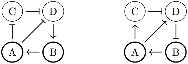
Figure 2. U-switch of network N. Original network N on the left with set U = {A, B} in bold. The network σ^U(N) on the right.

For any choice of U, the U-switch is a switching homomorphism and an involution; therefore, it is a switching isomorphism. In Naserasr et al. [27], it was shown that any switching homomorphism is a U-switch followed by an edge sign preserving homomorphism. Basic properties of the switch operation are recorded in the following proposition.

Proposition 3.3. 1. If U = V then σ^U is the identity: σ^U = Id.

2. For all U ⊂ V, σ^U is an involution: σ^U ∘ σ^U = Id.

3. Given U, W ⊂ V, σ^U and σ^W commute: σ^U ∘ σ^W = σ^W ∘ σ^U.

4. Given U = {u₁, …, u_n} ⊂ V, ${\sigma }^U={\sigma }^{u_1}\circ \cdots \circ {\sigma }^{u_n}$.

4 Switch isomorphisms preserve network dynamics

In this section, we examine the relationship between the dynamics of network N and the switched network σ^U(N). Since the switch operation σ^U fixes the nodes V and edges E, and the set of parameter nodes $\mathcal{P}(N)$ does not depend on the edge signs, we have $\mathcal{P}(N)=\mathcal{P}({\sigma }^U(N))$.

Before we formulate the main result, we outline the main idea. Define bijection λ^U:X → X component-wise by

${\lambda }^U(x)={({\lambda }_u^U(x_u))}_{u\in V}{\lambda }_u^U(x_u)=\{\begin{array}{ll}{m}_u-x_u,& \text{ if }u\in U\\ x_u,& \text{ if }{x}_u\notin U.\end{array}$

That is, λ^U reflects the components X_u for each u ∈ U and is the identity on the components X_u for u ∉ U. Clearly, λ^U is an involution. Then, given ${\mathcal{F}}^0(·;p,N):X\to X$ at parameter $p\in \mathcal{P}(N)$, the map ${\mathcal{F}}^{0,U}:={\lambda }^U\circ {\mathcal{F}}^0\circ {\lambda }^U$ is isomorphic to ${\mathcal{F}}^0$. Therefore, both synchronous dynamics given by iterates of ${\mathcal{F}}^0$ and asynchronous dynamics given by $\mathcal{F}$ on STG are identical. The main result of this section precisely identifies the map on the parameter graph $D^U:\mathcal{P}(N)\to \mathcal{P}({\sigma }^U(N))$ such that ${\mathcal{F}}^{0,U}={\mathcal{F}}^0(·;D^U(p),{\sigma }^U(N))$. Importantly, we show that the map D^U is graph automorphism; that is, it maps not only nodes to nodes but also edges to edges.

Theorem 4.1. Given the U-switch σ^U, there is an induced isomorphism $D^U:\mathcal{P}(N)\to \mathcal{P}({\sigma }^U(N))$ and a bijection λ^U:X → X such that the the following diagram commutes

In other words, the dynamics of ${\mathcal{F}}^0(·;p,N)$ and ${\mathcal{F}}^0(·;D^U(p),{\sigma }^U(N))$ is conjugate at parameters related by D^U. The map λ^U is a graph isomorphism between the STG representing $\mathcal{F}(·;p,N)$ and the STG representing $\mathcal{F}(·;D^U(p),{\sigma }^U(N))$. Consequently, the Morse graphs MG(p) and MG(D^U(p)) are isomorphic and corresponding Morse nodes have the same label.

A consequence of Proposition 3.3(4) is that we need only to demonstrate that the diagram Equation 3 commutes in the case that U = {u} consists of a single node.

4.1 The dual parameter map D^U

Let u ∈ V be a node and $p_u=(f_u,{\theta }_u)\in \mathcal{P}(u)$ be a u-parameter. The dual parameter to p_u is defined to be q_u = (g_u, ϕ_u) where

$\begin{array}{cc}{\varphi }_u(v)=m_u+1-{\theta }_u(v)\text{ and }{g}_u^i(b)=\neg f_u^{m_u+1-i}(\neg b),& (4)\end{array}$

and m_u = |T(u)|. The reason we say q_u is the dual parameter to p_u is because $g_u^i$ is the dual Boolean function to $f_u^{m_u+1-i}$. There is a large literature on dualization of Boolean functions and its computational complexity. See, for example [54].

Define $d_u:\mathcal{P}(u)\to \mathcal{P}(u)$ to be the map from a u-parameter to its dual parameter. The following Lemma is a direct consequence of the definition of d_u.

Lemma 4.2. Given any u-parameter $p_u\in \mathcal{P}(u)$, its dual parameter $d_u(p_u)\in \mathcal{P}(u)$, that is, the map d_u is well-defined. Moreover, d_u is an involution: d_u ∘ d_u = Id.

Proof. We show that $d_u(p_u)\in \mathcal{P}(u)$. Clearly, ϕ_u is a valid order parameter. We now show that g_u satisfies the ordering condition (Equation 1). Since f_u satisfies the ordering condition, we have $f_u^1(\neg (b))\ge \cdots \ge f_u^{m_u}(\neg b)$ and therefore $\neg f_u^1(\neg b)\le \cdots \le \neg f_u^{m_u}(\neg b)$. By Definition 4, $g_u^1(b)\ge \cdots \ge g_u^{m_u}(b)$ so that g_u satisfies the ordering condition. Next, we show that $g_u^i$ is an MBF. Let b¹ ≺ b², which implies ¬b¹ ≻ ¬b². Since $f_u^{m_u+1-i}$ is an MBF, we have

$g_u^i(b^1)=\neg f_u^{m_u+1-i}(\neg b^1)\le \neg f_u^{m_u+1-i}(\neg b^2)=g_u^i(b^2).$

This shows $g_u^i$ is an MBF.

The second part of the Lemma follows by inspection.     □

We are now ready to define the parameter graph isomorphism corresponding to σ^U. Since σ^U fixes the nodes V and edges E, and the set of parameter nodes $\mathcal{P}(N)$ does not depend on the edge signs, we have $\mathcal{P}(N)=\mathcal{P}({\sigma }^U(N))$. Therefore, we will omit the network N from the argument of the parameter set $\mathcal{P}$ and the parameter graph PG.

Let U ⊂ V. The U-dual parameter map $D^U:\mathcal{P}\to \mathcal{P}$ is defined by

$D^U(p)={(D_u^U(p_u))}_{u\in V}{D}_u^U(p_u)=\{\begin{array}{ll}{d}_u(p_u),& \text{ if }u\in U\\ p_u,& \text{ if }u\notin U\end{array}.$

Proposition 4.3. The U-dual parameter map D^U is a graph automorphism of PG for all U ⊂ V.

Proof. By Lemma 4.2 d_u, is an involution on $\mathcal{P}(u)$. Since each component of D^U is either the identity on that component or given by d_u, D^U is an involution on $\mathcal{P}$ and hence a bijection. It remains to show that D^U preserves parameter graph adjacency.

Let $p=(f,\theta ),\overline{p}=(\overline{f},\overline{\theta })\in \mathcal{P}$ be adjacent parameters. Let q = (g, ϕ) = D^U((f, θ)) and $\overline{q}=(\overline{g},\overline{\varphi })=D^U((\overline{f},\overline{\theta }))$. Furthermore, let u be the unique node such that p_u and ${\overline{p}}_u$ are adjacent. For w ≠ u, $p_w={\overline{p}}_w$ and therefore $q_w={\overline{q}}_w$.

First suppose p_u and ${\overline{p}}_u$ are order adjacent. Then there is an adjacent transposition π such that

${\theta }_u=\pi \circ {\overline{\theta }}_u.$

If u ∉ U then ϕ_u = θ_u and ${\overline{\varphi }}_u={\overline{\theta }}_u$ so that q_u and ${\overline{q}}_u$ are order adjacent. If u ∈ U, then

${\varphi }_u=m_u+1-{\theta }_u=m_u+1-\pi \circ {\overline{\theta }}_u=\tau \circ {\overline{\varphi }}_u$

where τ(i): = m_u + 1 − π(m_u + 1 − i) is an adjacent transposition. Order adjacency of p_u and ${\overline{p}}_u$ implies $f=\overline{f}$ and thus $g=\overline{g}$, so we conclude q and $\overline{q}$ are order adjacent.

Finally, suppose p_u and ${\overline{p}}_u$ are logically adjacent. If u ∉ U then q_u = p_u and ${\overline{q}}_u={\overline{p}}_u$ so that q_u and ${\overline{q}}_u$ are logically adjacent.

If u ∈ U, then $\theta =\overline{\theta }$ and thus $\varphi =\overline{\varphi }$. Let i be the unique index and b₀ be the unique input such that $f_u^i(b_0)\ne {\overline{f}}_u^i(b_0)$. Then

$g_u^{m_u+1-i}(\neg b_0)=\neg f_u^i(b_0)\ne \neg {\overline{f}}_u^i(b_0)={\overline{g}}_u^{m_u+1-i}(\neg b_0)$

and for b ≠ b₀, $f_u^j(b)={\overline{f}}_u^j(b)$ so that

$g_u^{m_u+1-i}(\neg b)=\neg f_u^{m_u+1-i}(b)=\neg {\overline{f}}_u^{m_u+1-i}(b)={\overline{g}}_u^{m_u+1-i}(\neg b).$

Similarly for j ≠ i and any b

$g_u^{m_u+1-j}(\neg b)=\neg f_u^{m_u+1-j}(b)=\neg {\overline{f}}_u^{m_u+1-j}(b)={\overline{g}}_u^{m_u+1-j}(\neg b).$

We conclude that m_u + 1 − i is the unique index and ¬b₀ is the unique input such that $g_u^{m_u+1-i}(\neg b_0)\ne {\overline{g}}_u^{m_u+1-i}(\neg b_0)$ It follows that q and $\overline{q}$ are logically adjacent.

Since D^U is invertible and preserves both order and logical adjacency, D^U is an automorphism of PG.

     □

4.2 Preservation of dynamics

The difference between the target point map ${\mathcal{F}}_0$ for the network N and the network σ^U(N) is due to the dependence of the input map B^u (see the beginning of Section 2.3) on the edge signs δ. The following lemma relates the input map B^u(·;θ, δ) for N and the input map B^u(·;ϕ, σ^U(δ)) for σ^U(N). By Proposition 3.3(4), we need only consider the case U = {u}.

Lemma 4.4. Let, u ∈ V, $(f,\theta )\in \mathcal{P}$, and (g, ϕ) = D^{u}((f, θ)). Let η = σ^{u}(δ). Then for all w ∈ S(u),

$\begin{array}{cc}{B}_w^u(x;\theta ,\delta )=\neg B_w^u({\lambda }^{\left\{u\right\}}(x),\varphi ,\eta ).& (5)\end{array}$

For v ≠ u and all w ∈ S(v),

$\begin{array}{cc}{B}_w^v(x;\theta ,\delta )=B_w^v({\lambda }^{\left\{u\right\}}(x),\varphi ,\eta ).& (6)\end{array}$

Consequently,

$B^u(x;\theta ,\delta )=\neg B^u({\lambda }^{\left\{u\right\}}(x),\varphi ,\eta )\text{ and }{B}^v(x;\theta ,\delta )=B^v({\lambda }^{\left\{u\right\}}(x),\varphi ,\eta )$

for v ≠ u.

Proof. To simplify notation, let λ = λ^{u}.

First consider w ∈ S(u)\{u}. Since λ_w = Id and ϕ_w = θ_w, we have x_w < θ_w(u) if and only if λ_w(x_w) < ϕ_w(u). Equation (5) then follows after observing ${\delta }_w^u=-{\eta }_w^u$.

Next, we consider the case u ∈ S(u), that is, a self-edge. Note that for all v ∈ T(u),

$\begin{array}{ll}{x}_u<& {\theta }_u(v)\text{ implies }{\lambda }_u(x_u)=m_u-x_u\ge m_u+1-{\theta }_u(v)={\varphi }_u(v)\text{ and }\\ x_u\ge & {\theta }_u(v)\text{ implies }{\lambda }_u(x_u)=m_u-x_u<m_u+1-{\theta }_u(v)={\varphi }_u(v).\end{array}$

So, if u ∈ S(u), we have x_u < θ_u(u) if and only if x_u ≥ ϕ_u(u). Since ${\delta }_u^u={\eta }_u^u$, Equation (5) holds with w = u.

Now, suppose v ≠ u and w ∈ S(v). If w ≠ u, then λ_w = Id, ϕ_w = θ_w, and ${\eta }_w^v={\delta }_w^v$ implies Equation (6) holds. If w = u, then x_u < θ_u(v) holds if and only if

${\lambda }_u(x_u)=m_u-x_u\ge m_u+1-{\theta }_u(v)={\varphi }_u(v).$

Since ${\eta }_u^v=-{\delta }_u^v$, Equation (6) holds.     □

Proof of Theorem 4.1. By Proposition 3.3(4), it is sufficient to consider the case U = {u}. To simplify notation, we omit U as an argument of λ and D and let η = σ^U(δ). Let p = (f, θ) and (g, ϕ) = D(p) be the U-dual parameter.

Note that for v ≠ u, λ_v(x_v) = x_v, g_v = f_v, and, by Lemma 4.4 also B^v(x; θ, δ) = B^v(λ(x);ϕ, η). Therefore

$\begin{array}{c}\left|\left\{f_v^i(B^v(x;\theta ,\delta ))=1\right\}\right|=\left|\left\{g_v^i(B^v(\lambda (x);\varphi ,\eta ))=1\right\}\right|.\end{array}$

Consequently, if we denote ${\overline{x}}_v={\mathcal{F}}_v^0(x;p,N)$ then ${\lambda }_v({\overline{x}}_v)={\overline{x}}_v={\mathcal{F}}_v^0(\lambda (x);D(p),{\sigma }^U(N))$.

For node u itself, we have

$\begin{array}{l}\left|\left\{g_u^i(B^u(\lambda (x);\varphi ,\eta ))=1\right\}\right|=\left|\left\{f_u^{m_u+1-i}(\neg B^u(x;\theta ,\delta ))=0\right\}\right|\\ =m_u-\left|\left\{f_u^i(\neg B^u(x);\theta ,\delta )=1\right\}\right|\end{array}$

Consequently, with ${\overline{x}}_u={\mathcal{F}}_u^0(x;p,N)$,

${\mathcal{F}}_u^0(\lambda (x);D(p),{\sigma }^U(N))=m_u-{\mathcal{F}}_u^0(x;p,N)=m_u-{\overline{x}}_u={\lambda }_u({\overline{x}}_u).$

We have shown that λ^U verifies the conjugacy of ${\mathcal{F}}^0(·;p,N)$ and ${\mathcal{F}}^0(·;D^U(p),{\sigma }^U(N))$. Since $\mathcal{F}$ is derived from ${\mathcal{F}}^0$, it follows that λ^U is a graph isomorphism between STG(p, N) and STG(D^U(p), σ^U(N)). Since the STGs are isomorphic, the corresponding Morse graphs MG(p) and MG(D^U(p)) are isomorphic.     □

Remark 4.5. We want to point out that when U = V the set of all nodes, and the switch σ^V:N → N is the identity, the map $D^V:\mathcal{P}(N)\to \mathcal{P}(N)$ is not necessarily an identity automorphism on the parameter graph. As we will show in Section 8, the non-trivial automorphism D^V commutes with network projections defined in the next section.

5 Embedding

In this section, we address the question of when the dynamics of a subnetwork M agree with the dynamics of a larger network N. In fact, we find it more convenient to consider the inverse operation of removing (cutting) edges of a regulatory network N and study the effect on the dynamics.

Definition 5.1. Let N = (V, E, δ) be a regulatory network and $\overline{E}\subset E$ be a set of edges. The $\overline{E}$-cut of N is the network $C^{\overline{E}}(N):=(V,E\backslash \overline{E},\eta )$ where

${\eta }_u^v={\delta }_u^v\text{ if }u⊸v\notin \overline{E}.$

Alternatively, the map $I^{\overline{E}}:(V,E\backslash \overline{E},\eta )\to (V,E,\delta )$ satisfying $C^{\overline{E}}\circ I^{\overline{E}}=Id$ is a graph embedding (inclusion).

Since the cut operation only removes edges from N, our results will only explicitly apply when considering subnetworks M ⊂ N which have the same number of nodes. This assumption is convenient but not restrictive; if $M^{\prime }=(V^{\prime },E\backslash \overline{E},\eta )$ is a subnetwork of N with V′ ⊂ V, then we may add the missing nodes to M′ and consider $M=(V,E\backslash \overline{E},\eta )$. A missing node u ∈ V\V′ is completely disconnected from every other node; its state is fixed and plays no role in the dynamics. The dynamics of M′ and M are therefore identical.

We outline the main ideas of this section. Our goal is to relate the dynamics of network N at a parameter $p\in \mathcal{P}(N)$ with dynamics of subnetwork M at a parameter $q\in \mathcal{P}(M)$. In general, there is no such relationship as cutting edges will result in a change in dynamics. However, there are parameters p where one or more edges play no role in the dynamics. This happens when an edge is always active or always inactive, that is, one of the functions $f_u^v$ is constant. We call the corresponding edge u ⊸ v an output inessential edge. In the context of Boolean functions, such function $f_u^v$ has been called a degenerate [50] or non-observable [45] function. In addition, even when $f_u^v$ is non-constant, there may be cases where the edge u ⊸ v never independently causes a change at a target node. These will be called input inessential edges (see Definition 5.2 below). Clearly, at a parameter $p\in \mathcal{P}(N)$, there can be multiple edges of both types and we expect that cutting any subset of these edges would result in a network M with the same, or similar, dynamics.

However, there are important differences between these two types of edges. At a parameter where we remove only input inessential edges from N to create subnetwork M, the thresholds corresponding to cut edges do not affect the dynamics. As a consequence, the direction of edges in pairs of domains straddling such a threshold is the same and we can combine these pairs to a single domain (see Figure 3). This operation results in semi-conjugacy between the dynamics of X(N) and X(M), described in Theorem 5.4.

Figure 3

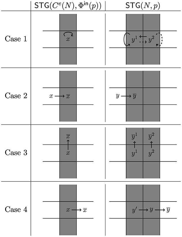
Figure 3. Maps of edges in STG(N, p) under the collapse map μ^e. The gray regions indicate (right) the layer $L_u^v$ about u ⊸ v in the state transition graph of N, and (left) the collapse map of the layer, ${\mu }^e(L_u^v)$, in the state transition graph of C^e(N). Each row represents a case from Proposition 6.1 that relates how the arrows in STG(N, p) are altered under the collapse map. In Case 1, either both undashed arrows or both dashed arrows are in STG(N, p), but not both.

On the other hand, at parameters where we remove output inessential edges, we find that the result can be strengthened in two important directions. First, the dynamics at $p\in \mathcal{P}(N)$ and the dynamics at the corresponding parameter $\Phi (p)\in \mathcal{P}(M)$ are conjugate, rather than semi-conjugate. In fact, we will identify a subgraph of X(N) that is isomorphic to X(M) (see Figure 4). More importantly, we show that the map $\Phi :\mathcal{P}(N)\to \mathcal{P}(M)$ has a collection of well-defined right inverses with disjoint images. Each inverse is a graph embedding of $\mathcal{P}(M)$ into a subgraph of $\mathcal{P}(N)$, and the images are mutually disjoint. Therefore not only dynamics, but parameterized dynamics of M is embedded inside parameterized dynamics of $\mathcal{P}(N)$. Furthermore, this dynamics is embedded multiple times within the parameterized dynamics of $\mathcal{P}(N)$.

Figure 4

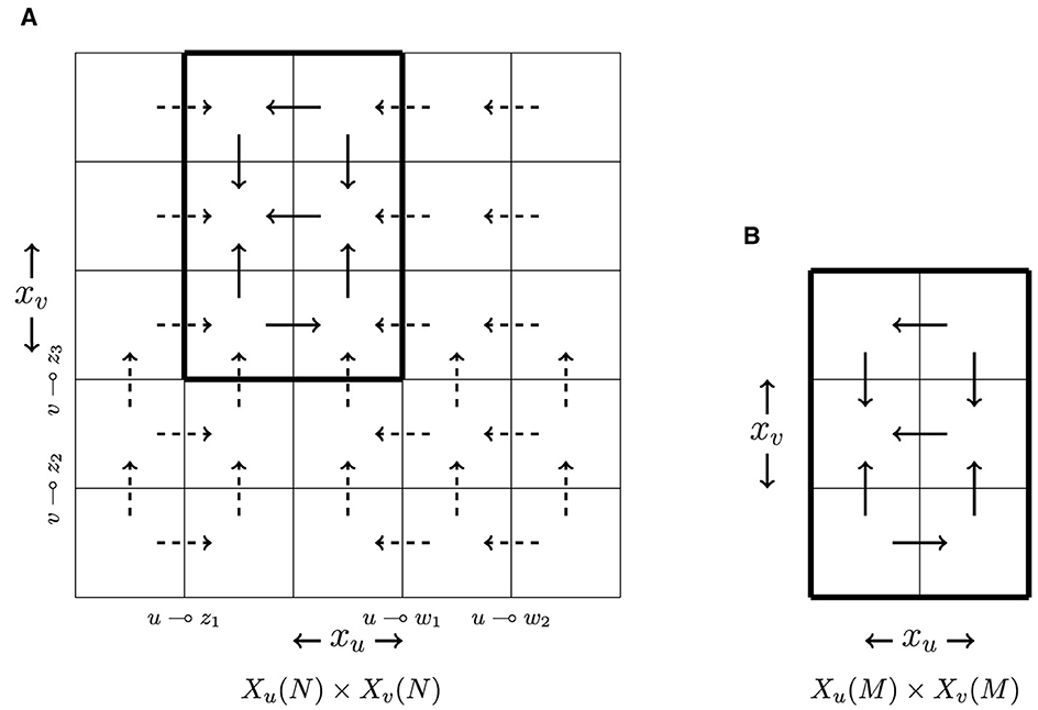
Figure 4. The (OFF,ON)-attractor X(OFF,ON). (A) Projection of X(N) into two dimensions; the subspace X_u(OFF,ON) × X_v(OFF,ON), outlined in bold, is an attractor in X(N). The dashed arrows between states in STG(N, p) are implied by the fact that $p\in \mathcal{P}(N;\text{OFF},\text{ON})$. The solid arrows represent transitions that are dependent on the specific choice of $p\in \mathcal{P}(N;\text{OFF},\text{ON})$. Boundaries corresponding to edges in OFF and ON are labeled with their corresponding edges. Here, T(u;ON) = {z₁}, T(u;OFF) = {w₁, w₂}, T(v;ON) = {z₂, z₃}, and T(v;OFF) = ∅. (B) STG(M, Φ(p,OFF,ON)) for network $M=C^{\overline{E}}(N)$ is isomorphic to the subgraph of STG(N, p) contained in X(OFF,ON).

We now proceed with precise description of inessential edges.

Definition 5.2. Let $p=(f,\theta )\in \mathcal{P}$ be a parameter.

• The edge u ⊸ v ∈ E is output-off inessential at p if $f_u^{{\theta }_u(v)}\equiv 0$, that is, when the monotone Boolean function corresponding to u ⊸ v is always off, and output-on inessential at p if $f_u^{{\theta }_u(v)}\equiv 1$, that is, when the monotone Boolean function corresponding to u ⊸ v is always on. If u ⊸ v is neither output-off nor output-on inessential, then u ⊸ v is output essential.

• The edge w ⊸ u ∈ E is input essential at p if there is an i ∈ {1, …, m_u} and a b ∈ 𝔹^S(u) such that $f_u^i(b)=\neg f_u^i(b+e^w)$ where e^w ∈ 𝔹^S(u) is defined by

$e_w^w=1e_v^w=0\text{ for }v\ne w.$

Otherwise, the edge w ⊸ u ∈ E is input inessential.

• An edge u ⊸ v ∈ E is essential at p if it is both input and output essential and inessential otherwise. We say that the parameter p is output or input inessential if there is an edge which is output or input inessential at p, respectively.

While the output inessential edges u ⊸ v transmit constant information to node v, the input inessential edge w ⊸ u does not affect the node u in the sense that if u changed state, there must be an input node w′ ≠ w that also changed state.

Example: To illustrate the input and output inessential edges consider PG(y) from Figure 1C. The essential parameters are II (logical function AND) and V (logical function OR). Functions I and VI are constant and thus both input and output inessential; I is output-off inessential, and VI is output-on inessential. Note that the function III copies the value of the input ¬X; this implies that the edge x ⊣ y is input essential, but the edge z → y is input inessential. Similarly, function IV makes x ⊣ y input inessential but z → y is input essential. At both parameters III and IV, the output edge y → z is output essential.

In parameter factor graph PG(x) in Figure 1A, the node B is essential, while both A and C are both input and output inessential.

Finally, in parameter graph PG(z) only the nodes 4 and 9 are essential, all others are inessential.

In the following exposition, it will be easier to consider the cutting of input inessential and output inessential edges independently, that is, $\overline{E}$ will either consist of a single input inessential edge or a set of output inessential edges. Since the cut edges $\overline{E}$ can be decomposed into these groups, and because we show in Proposition A4 that maps defined on these independent groups commute, the relationship between the dynamics of N and $C^{\overline{E}}(N)$ can be described for an arbitrary collection of inessential edges $\overline{E}$.

We define the set of parameter nodes in $p\in \mathcal{P}(N)$ where it is possible for the dynamics to be related to a parameter node $q\in \mathcal{P}(M)$ by cutting a single input inessential edge e or a set of output inessential edges. For a given set of nodes S ⊂ V let T(u; S) = T(u)∩S.

Definition 5.3. Let e ∈ E be an edge u ⊸ v. Then

• Let ${\mathcal{P}}^{\text{in}}(e)\subset \mathcal{P}(N)$ be a set of parameters at which the edge e is input inessential.

• Let $\mathcal{P}(\text{OFF},\text{ON})\subset \mathcal{P}(N)$ be the set of parameters such that

1. each edge e ∈ OFF is output-off inessential at p,

2. each edge e ∈ ON is output-on inessential at p, and

3. for every u ∈ V, the edges in ON are ranked first by θ and the edges in OFF are ranked last by θ:

$\begin{array}{cc}{\theta }_u(\text{T}(u;\text{ON}))<{\theta }_u(\text{T}(u;E\backslash (\text{OFF}\bigsqcup \text{ON}))<{\theta }_u(\text{T}(u;\text{OFF})).& (7)\end{array}$

Note that ${\mathcal{P}}^{\text{OFF}}(e)\cap {\mathcal{P}}^{\text{ON}}(e)=\varnothing$, but that ${\mathcal{P}}^{\text{in}}(e)\cap \mathcal{P}(\text{OFF},\text{ON})$ may not be empty as there can be parameters at which a given edge e is both input and output inessential. Note further that it is the last condition (3) for output inessential edges that motivated us to define $\mathcal{P}(\text{OFF},\text{ON})$ for a set rather than for a single edge as in the input inessential case.

We define in Section 5.1 two projections. First,

${\Phi }^{in}(·;e):{\mathcal{P}}^{in}(e)\to \mathcal{P}(C^e(N))$

that relates parameters with the same dynamics when we cut a single input inessential edge $e\in \overline{E}$ from N. Second, consider the case when $\overline{E}=\text{OFF}\bigsqcup \text{ON}$ consists of (several) output inessential edges. We define a projection map

$\Phi (·;\text{OFF},\text{ON}):\mathcal{P}(\text{OFF},\text{ON})\to \mathcal{P}(C^{\text{OFF}\bigsqcup \text{ON}}(N))$

that relates parameters with the same dynamics when we cut a collection of output inessential edges. Importantly, as we show in Proposition 8.4, these two projections commute:

$\begin{array}{c}{\Phi }^{in}(·;e)\circ \Phi (·;\text{OFF},\text{ON})=\Phi (·;\text{OFF},\text{ON})\circ {\Phi }^{in}(·;e)\\ {\Phi }^{in}(·;e)\circ {\Phi }^{in}(·;ê)={\Phi }^{in}(·;ê)\circ {\Phi }^{in}(·;e).\end{array}$

The following two theorems are the main results of this section, establishing a correspondence between the dynamics of the networks N and $C^{\overline{E}}(N)$.

Theorem 5.4. Let e ⊂ E be an input inessential edge and $p\in {\mathcal{P}}^{\text{in}}(e)$ be an input inessential parameter. The projection Φⁱⁿ(·;e) satisfies the following.

1. There is a surjective map μ^e:X(N) → X(C^e(N)) such that the target point map ${\mathcal{F}}^0(·;{\Phi }^{in}(p),C^e(N))$ is semi-conjugate to ${\mathcal{F}}^0(·;p,N)$, that is, the following diagram commutes

2. The Morse graph MG(Φⁱⁿ(p), C^e(N)) is a subgraph of MG(p, N).

3. There is a one-to-one correspondence between the Morse nodes labeled FP that contain fixed points of the dynamics.

The semi-conjugacy of the dynamics is strengthened to conjugacy when every cut edge is output inessential so that $\overline{E}=\text{OFF}\bigsqcup \text{ON}.$

Theorem 5.5. Let $\overline{E}=\text{OFF}\bigsqcup \text{ON}\subset E$ and $p\in \mathcal{P}(\text{OFF},\text{ON})$ be an output inessential parameter. The projection Φ(·;OFF,ON) has a collection of right inverses ${\{\text{Ψ}(·;{\zeta }^Q,{\zeta }^R,\widehat{f})\}}_{({\zeta }^Q,{\zeta }^R,\widehat{f})}$ indexed by order parameters ζ^Q ∈ Θ(OFF) and ζ^R ∈ Θ(ON), and anchoring logics $\widehat{f}\in \mathcal{A}(N;\text{OFF},\text{ON})$ (Definition 7.5). For each choice $({\zeta }^Q,{\zeta }^R,\widehat{f})$

1. The target point map ${\mathcal{F}}^0(·;\Phi (p),C^{\overline{E}}(N))$ is conjugate to ${\mathcal{F}}^0(·;p,N)$ restricted to a subset X(OFF,ON) ⊂ X(N), that is, the following diagram commutes

Consequently, the map ρ^OFF,ON is an embedding of the state transition graph $\text{STG}(X(C^{\overline{E}}(N)),\Phi (p))$ into STG(X(N), p).

2. The Morse graph $\text{MG}(\Phi (p),C^{\overline{E}}(N))$ is a subgraph of MG(p, N). The only Morse nodes of MG(p, N) that do not correspond to a node in $\text{MG}(\Phi (p),C^{\overline{E}}(N))$ must be labeled PC and have a successor node in the Morse graph.

3. $\Phi (·;\text{OFF},\text{ON})\circ \text{Ψ}(·;{\zeta }^Q,{\zeta }^R,\widehat{f})=Id$;

4. $\text{Ψ}(·;{\zeta }^Q,{\zeta }^R,\widehat{f}):\mathcal{P}(C^{\overline{E}}(N))\to \mathcal{P}(N;\text{OFF},\text{ON})$ is a graph embedding.

In the remainder of the section, we will build the machinery for the proofs of Theorems 5.4, 5.5, to be found in Sections 6, 7, respectively.

5.1 The projection maps Φⁱⁿ and Φ

In this section, we define the projection maps

$\begin{array}{r}{\Phi }^{in}(·;e)):{\mathcal{P}}^{in}(e)\to \mathcal{P}(C^e(N))\\ \Phi (·;\text{OFF},\text{ON}):\mathcal{P}(\text{OFF},\text{ON})\to \mathcal{P}(C^{\overline{E}}(N)).\end{array}$

where the set of cut edges is $\overline{E}=\left\{e\right\}$ in the first case and $\overline{E}=\text{OFF}\bigsqcup \text{ON}$ in the second.

Given a subset of edges E′ ⊂ E, it is useful to define

$\begin{array}{c}\text{S}(u;E^{\prime }):=\left\{w\in \text{S}(u;N)|w⊸u\in E^{\prime }\right\}\text{ and }\end{array}$

$\begin{array}{rr}\text{T}(u;E^{\prime }):=\left\{v\in \text{T}(u;N)|u⊸v\in E^{\prime }\right\}& (9)\end{array}$

to be the set of source and target nodes of u which correspond to edges in E′, respectively.

To define either of the projections Φⁱⁿ, Φ for given parameter $p=(f,\theta )\in \mathcal{P}(N)$, we need to construct a subnetwork parameter $(g,\varphi )\in \mathcal{P}(C^{\overline{E}}(N))$.

The idea for the construction of the order parameter ϕ_u from θ_u is simple: We define ϕ_u so that the ordering of the uncut edges is the same as the ordering given by θ_u. Explicitly, for (g, ϕ) = Φ((f, θ);OFF,ON) where the set $\overline{E}=\text{OFF}\bigsqcup \text{ON}$ could have more than one element, we proceed as follows. For each u ∈ V and v ∈ T(u), define

$\begin{array}{cc}{\#}_u(v):=\left|\left\{i<{\theta }_u(v)|{\theta }_u^{-1}(i)\in \text{T}(u;\overline{E})\right\}\right|& (10)\end{array}$

to be the number of out-edges of u with rank less than θ_u(v) which are cut from N. The u-order parameter is defined by

$\begin{array}{cc}{\varphi }_u(v)={\theta }_u(v)-{\#}_u(v).& (11)\end{array}$

For (g, ϕ) = Φⁱⁿ((f, θ);e) we proceed in the same way realizing that $\overline{E}=\left\{e\right\}$ has a single element.

To construct a $g\in \mathcal{L}(C^{\overline{E}}(N))$ from $f\in \mathcal{L}(N)$, we will replace inputs that correspond to edges in $\overline{E}$ in function f by constant inputs. If the edge is input inessential at parameter p, we can replace this input by either 0 or 1; since the edge is input inessential, the value of g does not depend on the value that is selected. On the other hand, if the edge is output inessential, the values of these constants depend on whether the cut edge e = (w ⊸ u) belongs to set ON, whether it belongs to set OFF, and the sign of the edge. We start with this latter case. Assume $\overline{E}=\text{OFF}\bigsqcup \text{ON}$ and let $p=(f,\theta )\in \mathcal{P}(\text{OFF},\text{ON})$. We construct a logic parameter $g\in \mathcal{L}(C^{\overline{E}}(N))$ from f as follows. For each $w\in \text{S}(u;\overline{E})$, let

$\begin{array}{cc}{\beta }_w^u(\text{OFF},\text{ON}):=\{\begin{array}{l}0,\text{ if }{\delta }_w^u=1\text{ and }w\to u\in \text{OFF}\\ \text{ or }{\delta }_w^u=-1\text{ and }w⊣u\in \text{ON}\\ 1,\text{ if }{\delta }_w^u=1\text{ and }w\to u\in \text{ON}\\ \text{ or or }{\delta }_w^u=-1\text{ and }w⊣u\in \text{OFF}\end{array}.& (12)\end{array}$

That is, ${\beta }_w^u$ is the constant input from w to u based on whether the edge w ⊸ u ∈ OFF and therefore inactive or w ⊸ u ∈ ON and therefore active. Let ${\beta }^u={({\beta }_w^u)}_{w\in \text{S}(u;\overline{E})}$ be the collection of these inputs. The function $g_u^{{\varphi }_u(v)}$ is constructed by evaluating the function $f_u^{{\theta }_u(v)}$. In general, there are fewer inputs to g_u then to f_u. So, for a given input to g_u, its value is computed by evaluating f_u on the same input with missing inputs replaced with β^u. For each $b\in \text{S}(u;C^{\overline{E}}(N))$, we define

$\begin{array}{cc}{g}_u^{{\varphi }_u(v)}(b):=f_u^{{\theta }_u(v)}(b,{\beta }^u).& (13)\end{array}$

The (OFF,ON)-projection of $(f,\theta )\in \mathcal{P}(N)$ onto $\mathcal{P}(C^{\overline{E}}(N))$ is defined to be

$\Phi ((f,\theta );\text{OFF},\text{ON}):=(g,\varphi ).$

Assume now $\overline{E}=\left\{e\right\}$ and let $p=(f,\theta )\in {\mathcal{P}}^{in}(e)$. Let e = (w ⊸ u). Let ${\beta }_w^u\in \left\{0,1\right\}$ be arbitrary. We then define $g_u^{{\varphi }_u(v)}(b)$ as in Equation 13. Because w ⊸ u is input inessential, $g_u^{{\varphi }_u(v)}$ is independent of the choice of ${\beta }_w^u$. Then, the Φⁱⁿ(·;e) projection of $(f,\theta )\in \mathcal{P}(N)$ onto $\mathcal{P}(C^e(N))$ is defined to be

${\Phi }^{in}((f,\theta );e):=(g,\varphi ).$

Remark 5.6. An astute reader will notice that the definition of Φⁱⁿ and Φ only differs in choice of fixed input β; in Equation 12 for output inessential parameters, the choice is dictated by the membership of the cut edge in ON vs. OFF, while for input inessential parameters β can have arbitrary value since this value does not affect the target node. This can be expressed by

$\begin{array}{ll}{\Phi }^{in}(p;e)=\Phi (p;\left\{e\right\},\varnothing )=\Phi (p;\varnothing ,\left\{e\right\}),& (14)\end{array}$

that is, the Φⁱⁿ(p; e) agrees with Φ(p) if we chose to designate the edge e as either belonging to ON or to OFF set of edges.

Remark 5.7. Observe that although we designated the domain of Φ as the set of parameters in $\mathcal{P}(\text{OFF},\text{ON})$, the map Φ is well-defined on the entire parameter space $\mathcal{P}(N)$. Using relationship (Equation 14), the map Φⁱⁿ is also defined on $\mathcal{P}(N)$. However, there is only a well-predicted relationship between the dynamics of N and $C^{\overline{E}}(N)$ for $\overline{E}$-cuts that are composed entirely of inessential edges. For $\overline{E}$-cuts involving essential edges, the relationship between the dynamics of N and the dynamics of the cut network is unknown.

In Section 8, we provide some algebraic properties of Φ. In particular, in Theorem 8.1, we show that the V-dual automorphism $D^V:\mathcal{P}(N)\to \mathcal{P}(N)$, which is a result of the switch map σ^V that changes the signs of all edges incident to all nodes, commutes with Φ when the identities of OFF and ON edges are switched: letting $\overline{E}={\overline{E}}_1\bigsqcup {\overline{E}}_2$,

$D^V\circ \Phi (·;{\overline{E}}_1,{\overline{E}}_2)=\Phi (·;{\overline{E}}_2,{\overline{E}}_1)\circ D^V.$

We also prove that Φⁱⁿ(·;e) commutes with D^V.

6 Input inessential parameters

6.1 Proof of Theorem 5.4

Recall that ${\mathcal{P}}^{\text{in}}(e)\subset \mathcal{P}(N)$ denotes the set of parameters p such that the edge e = u ⊸ v is input inessential. Define the layer $L_u^v\subset X(N)$

$L_u^v:=\left\{x\in X|x_u\in \left\{{\theta }_u(v)-1,{\theta }_u(v)\right\}\right\}$

to be the set of states which border the threshold corresponding to u ⊸ v. Note that $L_u^v$ has “thickness” 2 in u direction as all states x have x_u with one of two values. See the gray double rectangles in the right column of Figure 3 as an illustration of a layer surrounding a threshold.

Given an edge e = u ⊸ v, let μ^e:X(N) → X(C^e(N)) be the map which collapses $L_u^v$ to a thickness 1 layer with single u-state:

$\begin{array}{c}{\mu }^e(·;\theta ):={({\mu }_w^e)}_{w\in V}{\mu }_w^e(x_w)=x_w\text{ for }w\ne u\\ {\mu }_u^e(x_u):=\{\begin{array}{ll}{x}_u,& \text{ if }{x}_u<{\theta }_u(v)\\ x_u-1,& \text{ if }{x}_u\ge {\theta }_u(v).\end{array}\end{array}$

An illustration of this collapse is given by comparing the single gray rectangles in the left column of Figure 3 to the double gray rectangles in the right column. The left column is a portion of the state space of C^e(N), while the right column is a portion of the state space of N.

In Proposition 8.3, we show that μ^e commutes with λ^V, the reflection bijection defined at the beginning of Section 4, as is suggested by Theorem 8.1 which says Φⁱⁿ and D^V commute.

Proof of Theorem 5.4 (1). Let $p=(f,\theta )\in {\mathcal{P}}^{\text{in}}(e)$ with e = u ⊸ v. To simplify notation, let M = C^e(N).

For w ∈ V\{u, v}, p_w = q_w and ${\mu }_w^e$ is the identity so that the target point maps commute with the collapse map

${\mu }_w^e\circ {\mathcal{F}}_w^0(·;p,N)={\mathcal{F}}_w^0(·;q,M)\circ {\mu }_w^e.$

Next, we consider node u. To show that the input maps B^u to node u (used to define the target point map in Section 2.3) for both networks agree, let x ∈ X and w ∈ S(u; M), that is, there is an edge w ⊸ u. If w ≠ u, then ${\mu }_w^e(x_w)=x_w$ and θ_w = ϕ_w so that $B_w^u(x;\theta ,N)=B_w^u({\mu }^e(x);\varphi ,M)$. If w = u, that is, there is a self-edge u ⊸ u, then, recalling the definition of ϕ_u Equation 11 and comparing to ${\mu }_u^e$, we have ${\varphi }_u(u)={\mu }_u^e({\theta }_u(u))$. Consequently,

$B_u^u(x;\theta ,N)=B_u^u({\mu }^e(x);\varphi ,M).$

If v = u, we need to compare the logic parameters f_u and g_u. By assumption, $f_u^i(b)$ is independent of b_u since u ⊸ v is input inessential at p. Since the inputs to f_u and g_u agree,

$\begin{array}{cc}{f}_u^{{\theta }_u(z)}(B^u(x;\theta ,N))=g_u^{{\varphi }_u(z)}(B^u({\mu }^e(x);\varphi ,M))\text{ for all }z\in \text{T}(u;N)\backslash \left\{v\right\}.& (15)\end{array}$

If $f_u^{{\theta }_u(v)}(B^u(x;\theta ,N))=0$, then Equation 15 and the definition of ${\mathcal{F}}^0$ imply that the u target point maps agree on x and μ^e(x), that is, ${\mathcal{F}}_u^0(x;p,N)={\mathcal{F}}_u^0({\mu }^e(x);q,M)$. Moreover, $f_u^{{\theta }_u(v)}(B^u(x;\theta ,N))=0$ implies ${\mathcal{F}}_u^0(x;p,N)<{\theta }_u(v)$, so that ${\mathcal{F}}_u^0(x;p,N)={\mu }_u^e({\mathcal{F}}_u^0(x;p,N))$. Similarly, if $f_u^{{\theta }_u(v)}(B^u(x;\theta ,n))=1$, then

${\mathcal{F}}_u^0({\mu }^e(x);q,M)={\mathcal{F}}_u^0(x;p,N)-1={\mu }_u^e({\mathcal{F}}_u^0(x;p,N)),$

as desired.

Finally, we consider node v, assuming v ≠ u. For all w ≠ u, ${\mu }_w^e$ is the identity and ϕ_w = θ_w, so that $B_w^v(x;\theta ,N)=B_w^v({\mu }^e(x);\varphi ,M)$. Since f_v(b) is independent of b_u, we have

$f_v(B^v(x;\theta ,N))=g_v(B^v({\mu }^e(x);\varphi ,M))$

which implies ${\mu }_v^e({\mathcal{F}}_v^0(x;p,N))={\mathcal{F}}_v^0({\mu }^e(x);q,M)$ for all x ∈ X since ${\mu }_v^e$ is the identity. This completes the proof.

     □

Theorem 5.4 (2) follows from the semi-conjugacy: For any path $\bar{\tau }$ in X(C^e(N)), there is at least one path τ in X(N) with ${\mu }^e(\tau )=\bar{\tau }$.

To prove Theorem 5.4 (3), we need the following Proposition that shows that most of the edges in STG(N, p) can be recovered from STG(C^e(N), Φⁱⁿ(p)). Each case in the proposition is illustrated in Figure 3.

Proposition 6.1. Consider a single edge $\overline{E}=\left\{e=u⊸v\right\}$. Let $p\in {\mathcal{P}}^{\text{in}}(N;e)$, and q = Φⁱⁿ(p; e). Let $x\to \overline{x}\in \text{STG}(C^e(N),q)$. If $x,\overline{x}\notin {\mu }^e(L_u^v)$, then there are unique $y,\overline{y}\in X(N)$ with μ^e(y) = x and ${\mu }^e(\overline{y})=\overline{x}$ such that $y\to \overline{y}\in \text{STG}(N,p)$.

On the other hand, if $x\in {\mu }^e(L_u^v)$ or $\overline{x}\in {\mu }^e(L_u^v)$, then there are four cases.

1. If $x=\overline{x}$, then there there are exactly two y¹, y² ∈ X(N) with μ^e(y¹) = μ^e(y²) = x. Either y¹ → y², y² → y² ∈ STG(N, p) or y² → y¹, y¹ → y¹ ∈ STG(N, p).

2. If $x\notin {\mu }^e(L_u^v)$, then there is a unique edge $y\to \overline{y}\in \text{STG}(N,p)$ with μ^e(y) = x and ${\mu }^e(\overline{y})=\overline{x}$.

3. If $x,\overline{x}\in {\mu }^e(L_u^v)$ and $x\ne \overline{x}$, then there are two edges $y^i\to {\overline{y}}^i\in \text{STG}(N,p)$ with μ^e(yⁱ) = x and ${\mu }^e({\overline{y}}^i)=\overline{x}$ for i = 1, 2.

4. If $x\in {\mu }^e(L_u^v)$ and $\overline{x}\notin {\mu }^e(L_u^v)$, then there is a unique edge $y\to \overline{y}\in \text{STG}(N,p)$ with μ^e(y) = x and ${\mu }^e(\overline{y})=\overline{x}$. In addition, the state $y^{\prime }=y-(\overline{x}-x)$ has an edge y′ → y ∈ STG(N, p).

Proof. First suppose $x,\overline{x}\notin {\mu }^e(L_u^v)$ and $x\ne \overline{x}$. We start by noting that the map ${\mu }_w^e$ for w ≠ u is an identity on a finite set X_w and it is strictly monotone in that it satisfies

$\begin{array}{cc}\eta {\mu }_w^e(z_w^1)>\eta {\mu }_w^e(z_w^2)\iff \eta z_w^1>\eta z_w^2& (16)\end{array}$

for η ∈ {±1}. Furthermore, ${\mu }_u^e$, which is not an identity, satisfies (Equation 15) for all pairs $z^1,z^2\notin L_u^v$, and satisfies the forward implication in Equation 15 when $z^1\in L_u^v$ or $z^2\in L_u^v$.

Since μ^e is injective on $X(N)\backslash L_u^v$, there are unique $y,\overline{y}\in X(N)$ with μ^e(y) = x and ${\mu }^e(\overline{y})=\overline{x}$. Since $\overline{x}\in \mathcal{F}(x;q,C^e(N))$, there is a unique node w ∈ V (recall N = (V, E, δ)) and η ∈ {±1} with ${\overline{x}}_w=x_w+\eta$ and therefore ${\overline{y}}_w=y_w+\eta$. Applying Theorem 5.4 1 and Definition 2.2, we have

$\begin{array}{cc}\eta {\mu }_w^e({\mathcal{F}}_w^0(y;p,N))=\eta {\mathcal{F}}_w^0(x;q,C^e(N))>\eta x_w=\eta {\mu }_w^e(y_w).& (17)\end{array}$

Using Equation 15 with $z_w^1={\mathcal{F}}_w^0(y;p,N)$ and $z_w^2=y_w$, we conclude that

$\eta {\mathcal{F}}_w^0(y;p,N))>\eta y_w,$

which implies $y\to \overline{y}\in \text{STG}(N,p)$ as desired.

To complete the first claim of the proof, now suppose $x,\overline{x}\notin {\mu }^e(L_u^v)$ and $x=\overline{x}$. Since μ^e is injective on $X(N)\backslash L_u^v$, there is a unique y ∈ X(N) with μ^e(y) = x. By Definition 2.2,

${\mathcal{F}}^0(x;q,C^e(N))=x.$

Since the target point ${\mathcal{F}}^0(x;q,C^e(N))\notin {\mu }^e(L_u^v)$, the map μ^e is injective on ${\mathcal{F}}^0(y;p,N)$, and therefore by Theorem 5.4 (1), we have

${\mu }^e({\mathcal{F}}^0(y;p,N))={\mathcal{F}}^0(x;q,C^e(N))=x={\mu }^e(y),$

implying ${\mathcal{F}}^0(y;p,N)=y$, which indicates a self-edge at y ∈ STG(N, p) as desired.

Next, we consider the four cases of $x\in {\mu }^e(L_u^v)$ or $\overline{x}\in {\mu }^e(L_u^v)$.

Case 1 ($\text{x}=\overline{x}$). The pre-image of x is exactly two states {y¹, y²} = (μ^e)⁻¹(x) with

$y_u^1+1={\theta }_u(v)=y_u^2\text{ and }{y}_w^1=y_w^2\text{ for }w\ne u.$

Since u ⊸ v is input inessential, ${\mathcal{F}}_v^0(y^1;p,N)={\mathcal{F}}_v^0(y^2;p,N)$. For w ≠ v, if w ∈ T(u; N), ${\theta }_u(w)<y_u^1$ if and only if ${\theta }_u(w)<y_u^2$ so that the inputs B^w(y¹; N) = B^w(y²; N). Consequently ${\mathcal{F}}_w^0(y^1;p,N)={\mathcal{F}}_w^0(y^2;p,N)$. Since this holds for all nodes, ${\mathcal{F}}^0(y^1;p,N)={\mathcal{F}}^0(y^2;p,N)$. We also have

${\mu }^e({\mathcal{F}}^0(y^i;p,N))={\mathcal{F}}^0(x;q,C^e(N))=x$

so that either ${\mathcal{F}}^0(y^i;p,N)=y^1$ for both i = 1, 2, or ${\mathcal{F}}^0(y^i;p,N)=y^2$ for both i = 1, 2. This shows exactly one of y¹ → y², y² → y² ∈ STG(N, p) or y² → y¹, y¹ → y¹ ∈ STG(N, p) holds.

Case 2 ($\text{x}\notin {\mu }^e(L_u^v)$ and $\overline{x}\in {\mu }^e(L_u^v)$). There is a unique y with μ^e(y) = x. Let w be the unique node with ${\overline{x}}_w=x_w+\eta$ where η ∈ {±1}. Then by Theorem 5.4 (1) and Definition 2.2, the Equation (17) holds. Using Equation (16) this implies that $\eta {\mathcal{F}}_w^0(y;p,N)>\eta y_w$ so there is an edge $y\to \overline{y}\in \text{STG}(N,p)$ with ${\overline{y}}_w=y_w+\eta$ and thus ${\mu }^e(\overline{y})=\overline{x}$.

Case 3 ($\text{x},\overline{x}\in {\mu }^e(L_u^v)$ and $\text{x}\ne \overline{x}$). Let w be the unique node with ${\overline{x}}_w=x_w+\eta$ where η ∈ {±1}. Note that we must have w ≠ u (see Figure 3). The pre-image of x and $\overline{x}$ each consist of two states, {y¹, y²} = (μ^e)⁻¹(x) and $\left\{{\overline{y}}^1,{\overline{y}}^2\right\}={({\mu }^2)}^{-1}(\overline{x})$ with

$y_u^1+1={\overline{y}}_u^1+1={\theta }_u(v)=y_u^2={\overline{y}}_u^2.$

Then, for both i = 1, 2, we have

$\eta {\mu }_w^e({\mathcal{F}}_w^0(y^i;p,N))=\eta {\mathcal{F}}_w^0(x;q,C^e(N))>\eta x_w=\eta {\mu }_w^e(y^i).$

Using Equation 15 applied to w ≠ u we have $\eta {\mathcal{F}}_w^0(y^i;p,N)>\eta y^i$ so that $y^i\to {\overline{y}}^i\in \text{STG}(N,p)$.

Case 4 ($\text{x}\in {\mu }^e(L_u^v)$ and $\overline{x}\notin {\mu }^e(L_u^v)$). There is a unique $\overline{y}\in X(N)$ with ${\mu }^e(\overline{y})=\overline{x}$ and two states $y^1,y^2\in L_u^v$ with μ^e(yⁱ) = x. Let η ∈ {±1} such that ${\overline{x}}_u=x+\eta$. For both i = 1, 2, we have

$\begin{array}{cc}\eta {\mu }_u^e({\mathcal{F}}_u^0(y^i;p,N))=\eta {\mathcal{F}}_u^0(x;q,C^e(N))>\eta x_u=\eta {\mu }_u^e(y^i).& (18)\end{array}$

Let ${\tilde{y}}^i\in X(N)$ be the state defined by

${\tilde{y}}_u^i=y_u^i+\eta {\tilde{y}}_w^i=y_w^i\text{ for }w\ne u.$

Equation (18) together with Equation (16) implies that $y^i\to {\tilde{y}}^i\in \text{STG}(N,p)$. For one choice of i, say i = 1, ${\tilde{y}}^1\in L_u^v$ so that ${\tilde{y}}^1=y^2$. On the other hand, ${\tilde{y}}^2\notin L_u^v$ and ${\mu }^e({\tilde{y}}^2)=\overline{x}$. Set $\overline{y}:={\tilde{y}}^2$, y: = y², and y′ = y¹. Noting that ${(\overline{x}-x)}_u=\eta$ and ${(\overline{x}-x)}_w=0$ for w ≠ u, we have $y^{\prime }=y-(\overline{x}-x)$ (see Figure 3).     □

Theorem 5.4 (3) is obtained from Proposition 6.1 as follows. When the Morse graph $MG(\Phi (p),C^{\overline{E}}(N))$ has an FP at state $x\notin L_u^v$, then there is unique y with ${\mu }^{\overline{E}}(y)=x$ which is an FP in MG(p, N). On the other hand, if $x\in L_u^v$, then Case 1 of Proposition 6.1 shows that there is a FP y in MG(p, N) with ${\mu }^{\overline{E}}(y)=x$.

7 Output inessential parameters

7.1 The projection map Φ preserves dynamics

In this section, we begin the proof of Theorem 5.5 with the proof of point (1). Recall that an assumption of the theorem is that the $\overline{E}$-cut is composed entirely of output inessential edges, some of which may also be input inessential. The following definition identifies the attracting region X(OFF,ON) ⊂ X(N), which will turn out to be isomorphic to $X(C^{\overline{E}}(N))$.

Definition 7.1. Let $\overline{E}=\text{OFF}\bigsqcup \text{ON}\subset E$ and $p=(f,\theta )\in \mathcal{P}(N;\text{OFF},\text{ON})$. The (OFF,ON)-attractor of the STG X(N) is the subset X(OFF,ON) ⊂ X(N) given by

$X(\text{OFF},\text{ON}):={\displaystyle \prod _{u\in V}}{X}_u(\text{OFF},\text{ON})$

where for each network node u ∈ V

$\begin{array}{c}{X}_u(\text{OFF},\text{ON})\\ :=\left\{\left|\text{T}(u;\text{ON})\right|,\left|\text{T}(u;\text{ON})\right|+1,\dots ,\left|\text{T}(u)\right|-\left|\text{T}(u;\text{OFF})\right|\right\},\end{array}$

using Equation (9).

Note that X(OFF,ON) consists of the set of contiguous states x such that the value of $f_u^v(B^u(x))=0$ for all edges e:u ⊸ v with e ∈ OFF and the value of $f_u^w(B^u(x))=1$ for all edges e:u ⊸ w with e ∈ ON (see Figure 4). Note that in the Figure 4, the edge u ⊸ v corresponding to the smallest threshold θ_u(v) = 1 of u belongs to ON, while the two edges that correspond to largest two thresholds belong to OFF. As a result, the values of the multi-valued function g_u and the target point map ${\mathcal{F}}_u^0$ lie within the u-projection of the outlined area X_u(OFF,ON). A similar argument for the v-direction implies that all components of ${\mathcal{F}}^0$ lie in X_v(OFF,ON). Therefore, the asynchronous dynamics of $\mathcal{F}$ is attracted to X(OFF,ON), as indicated by the arrows.

As suggested by the name, for $p\in \mathcal{P}(\text{OFF},\text{ON})$, the (OFF,ON)-attractor is a global attractor of the multi-level dynamics. The next proposition proves this by showing that the image of the target point map ${\mathcal{F}}^0$ is contained in X(OFF,ON). As a consequence, all recurrent dynamics of $\mathcal{F}$ are contained in X(OFF,ON). We will make use of the input map B^u:X → B^S(u) introduced at the beginning of Section 2.3.

Proposition 7.2. Let $\overline{E}=\text{OFF}\bigsqcup \text{ON}\subset E$ and $p\in \mathcal{P}(N;\text{OFF},\text{ON})$. Then for all x ∈ X(N), ${\mathcal{F}}^0(x;p,N)\in X(\text{OFF},\text{ON})$.

Proof. Let u ∈ V and p = (f, θ). For each v ∈ T(u;ON), we have $f_u^{{\theta }_u(v)}\equiv 1$. Consequently, for any state x ∈ X,

${\mathcal{F}}_u^0(x;p)=\left|\left\{f_u^v(B^u(x))=1\right\}\right|\ge \left|\text{T}(u;\text{ON})\right|=min{X}_u(\text{OFF},\text{ON}).$

For each v ∈ T(u;OFF), we have $f_u^{{\theta }_u(v)}\equiv 0$ since u ⊸ v is output-off inessential at p. Consequently, for any state x ∈ X,

$\begin{array}{c}{\mathcal{F}}_u^0(x;p)=\left|\text{T}(u;N)\right|-\left|\left\{f_u^v(B^u(x))=0\right\}\right|\\ \le \left|\text{T}(u;N)\right|-\left|\text{T}(u;\text{OFF})\right|=max{X}_u(\text{OFF},\text{ON}).\end{array}$

Since u was arbitrary, this proves the proposition.     □

The idea of the proof of Theorem 5.5 (1) is to show that for the parameters in $\mathcal{P}(N;\text{OFF},\text{ON})$ the target points ${\mathcal{F}}^0(N)$ of the (OFF,ON)-attractor are the same as the target points ${\mathcal{F}}^0(C^{\overline{E}}(N))$ of the cut network after relabeling. An immediate consequence is that the STG for $C^{\overline{E}}(N)$ is graph isomorphic to the STG of the (OFF,ON)-attractor (Figure 4). We proceed to define the relabeling map ρ^OFF,ON, which appears in the commutative diagram (Equation 8).

Definition 7.3. The relabeling map ${\rho }^{\text{OFF},\text{ON}}:X(\text{OFF},\text{ON})\to X(C^{\overline{E}}(N))$ is

${\rho }^{\text{OFF},\text{ON}}(x)={({\rho }_u^{\text{OFF},\text{ON}}(x_u))}_{u\in V},{\rho }_u^{\text{OFF},\text{ON}}(x_u)=x_u-\left|\text{T}(u;\text{ON})\right|.$

We now show that the value of the input map for N at x agrees with the value of the input map for $C^{\overline{E}(N)}$ at ρ^OFF,ON(x).

Lemma 7.4. Let $\overline{E}=\text{OFF}\bigsqcup \text{ON}\subset E$, $(f,\theta )\in \mathcal{P}(N;\text{OFF},\text{ON})$, and (g, ϕ) = Φ((f, θ);OFF,ON) be the (OFF,ON)-projection of (f, θ). For each state x ∈ X(OFF,ON), u ∈ V, and w ∈ S(u; N)

$B_w^u(x;N)=\{\begin{array}{ll}{\beta }_w^u,& \text{ if }w⊸u\in \overline{E}\\ B_w^u({\rho }^{\text{OFF},\text{ON}}(x);C^{\overline{E}}(N)),& \text{ if }w⊸u\notin \overline{E}\end{array},$

where we suppressed the dependency ${\beta }_w^u={\beta }_w^u(\text{OFF},\text{ON})$ from Equation (12).

Proof. Let x ∈ X(OFF,ON). First suppose $w⊸u\in \overline{E}$. If w ⊸ u ∈ ON, then $(f,\theta )\in \mathcal{P}(N;\text{OFF},\text{ON})$ implies by Equation (7) that θ_w(u) ≤ |T(w;ON)| ≤ x_w. Consequently, by the definition of $B_w^u$ and ${\beta }_w^u$,

$B_w^u(x;\theta ,N)=\{\begin{array}{ll}0,& \text{ if }{\delta }_w^u=-1\\ 1,& \text{ if }{\delta }_w^u=1\end{array}={\beta }_w^u.$

If w ⊸ u ∈ OFF, then $(f,\theta )\in \mathcal{P}(N;\text{OFF},\text{ON})$ implies θ_w(u) > |T(w)|−|T(w;OFF)| ≥ x_w. Consequently, by the definition of $B_w^u$ and ${\beta }_w^u$,

$B_w^u(x;\theta ,N)=\{\begin{array}{ll}0,& \text{ if }{\delta }_w^u=1\\ 1,& \text{ if }{\delta }_w^u=-1\end{array}={\beta }_w^u.$

This completes the proof for the case $w⊸u\in \overline{E}$.

Now consider an edge $w⊸u\notin \overline{E}$. Since $(f,\theta )\in \mathcal{P}(N;\text{OFF},\text{ON})$, Equation (7) is satisfied and the edges in ON are ranked first by θ. This implies #_w(u) = |T(w;ON)|. In particular, we have

${\varphi }_w(u)={\theta }_w(u)-\left|\text{T}(w;\text{ON})\right|={\rho }_w^{\text{OFF},\text{ON}}({\theta }_w(u)).$

Since ${\rho }_w^{\text{OFF},\text{ON}}$ is monotonically increasing, we have x_w < θ_w(u) if and only if ${\rho }^{\text{OFF},\text{ON}}(x_w)<{\rho }^{\text{OFF},\text{ON}}({\theta }_w(u))={\varphi }_w(u)$. Since the sign of w ⊸ u in N is the same as the sign of w ⊸ u in $C^{\overline{E}}(N)$, the lemma holds in the case $w⊸u\notin \overline{E}$.     □

We are now ready to prove the main result of this subsection.

Proof of Theorem 5.5 (1). Let $p=(f,\theta )\in \mathcal{P}(N;\text{OFF},\text{ON})$ and q = (g, ϕ) = Φ(p;OFF,ON). To simplify notation, let ρ = ρ^OFF,ON and $M=C^{\overline{E}}(N)$. Let x ∈ X(OFF,ON). We need to show that

$\rho ({\mathcal{F}}^0(x;p,N))={\mathcal{F}}^0(\rho (x);q,M).$

First note that by Lemma 7.4 and the definition of g, we have

$f_u^{{\theta }_u(v)}(B^u(x);\theta ,N)=g_u^{{\varphi }_u(v)}(B^u(\rho (x));\varphi ,M)$

for each v ∈ T(u; M). Therefore, we have

$\begin{array}{c}{\rho }_u({\mathcal{F}}_u^0(x;p,N))=\left|\text{{}{f}_u^i(B^u(x;\theta ,N))=1\text{ | }i\in \{1,\dots ,|\text{T}(u;N)\left|\right\}\right|-\left|\text{T}(u;\text{ON})\right|\\ =\left|\text{T}(u;\text{ON})\right|+\left|\text{{}{g}_u^i(B^u(\rho (x);\varphi ,M)=1\text{ | }i\in \{1,\dots ,|\text{T}(u;M)|\}\right|-\left|\text{T}(u;\text{ON})\right|\\ =\left|\text{{}{g}_u^i(B^u(\rho (x);\varphi ,M)=1i\in \{1,\dots ,|T(u;M)|\left\}\right\}\right|={\mathcal{F}}^0(\rho (x);q,M)\end{array}$

where the second equality follows from the fact that $f_u^{{\theta }_u(v)}\equiv 1$ when v ∈ T(u;ON). This shows that the diagram (Equation 8) commutes so that the target point maps are conjugate.

Since the target point maps are conjugate and the asynchronous dynamics $\mathcal{F}$ are completely determined by the target point maps, we conclude that STG(X(M), q) is isomorphic to STG(X(OFF,ON), p), a subgraph of STG(X(N), p).

     □

Finally, we derive consequences of this result for the Morse graphs. Theorem 5.5 (1) implies that the only recurrent set of STG(X(N), p) which does not correspond to a recurrent set of STG(X(M), q) must be outside of the (OFF,ON)-attractor X(OFF,ON). Since X(OFF,ON) is the global attractor, these recurrent sets are represented as unstable Morse nodes in the Morse graph. Moreover, an FC cannot exist outside of X(OFF,ON) since all edges between states which are outside of X(OFF,ON) and adjacent in the u direction point toward X(OFF,ON). This argument proves Theorem 5.5 (2).

7.2 Embeddings of a subnetwork's parameter graph

In this section, we prove Theorem 5.5 (3) and (4) by constructing a collection of right inverses, {Ψ} to each projection Φ, each of which embeds the parameter graph $\text{PG}(C^{\overline{E}}(N))$ into PG(N) of the original network.

Given a parameter $q\in \mathcal{P}(C^{\overline{E}}(N))$, in order to construct a parameter p = (f, θ): = Ψ(q), we need to first determine the order parameter θ. However, the construction of θ requires a choice of an ordering for the edges that have been cut. We therefore let ζ^OFF ∈ Θ(OFF) and ζ^ON ∈ Θ(ON) be orderings of the sets OFF and ON, respectively. Let $\mathcal{P}(N;{\zeta }^{\text{OFF}},{\zeta }^{\text{ON}})\subset \mathcal{P}(N;\text{OFF},\text{ON})$ be the subset of output inessential parameters p = (f, θ) such that the order parameter θ agrees with the orderings given by ζ^OFF and ζ^ON:

$\begin{array}{cc}{\zeta }_u^{\text{ON}}(v)={\theta }_u(v)\text{ for }v\in \text{T}(u;\text{ON})& (19)\end{array}$

$\begin{array}{c}{\zeta }_u^{\text{OFF}}(v)={\theta }_u(v)-\left|\text{T}(u;E\backslash \text{OFF})\right|\text{ for }v\in \text{T}(u;\text{OFF}).\end{array}$

We next discuss how to construct a logic parameter $f\in \mathcal{L}(N;{\zeta }^{\text{OFF}},{\zeta }^{\text{ON}})$ for p = (f, θ) = Ψ((g, ϕ)).

We start by listing conditions we impose on map Ψ in order for it be the right inverse of Φ and to preserve parameter graph adjacency. Let $b^1\in {𝔹}^{\text{S}(u;C^{\overline{E}}(N))}$ and $b^2\in {𝔹}^{\text{S}(u;\overline{E})}$, that is, b¹ is an input vector with entries corresponding to the edges that exist in both networks and b² is an input with entries for edges that exist only in N and are being cut.

1. $f\in \mathcal{L}(N;{\zeta }^{\text{OFF}},{\zeta }^{\text{ON}})$ requires each edge in $\overline{E}$ to be output inessential: for each input b,

$f_u^{{\theta }_u(v)}(b)\equiv \{\begin{array}{ll}0,& \text{ if }u⊸v\in \text{OFF}\\ 1,& \text{ if }u⊸v\in \text{ON}\end{array}.$

2. Whenever u ⊸ v is an edge in both N and $C^{\overline{E}}(N)$, (recalling the definition of β from Equation 12) we will set

$\begin{array}{cc}{f}_u^{{\theta }_u(v)}(b^1,b^2)=g_u^{{\varphi }_u(v)}(b^1)\text{ when }{b}^2={\beta }^u,\text{ and }& (20)\end{array}$

$\begin{array}{ccc}{f}_u^{{\theta }_u(v)}(b^1,b^2)& \text{ is independent of }g\text{ when }{b}^2\ne {\beta }^u,& (21)\end{array}$

Condition (Equation 20) is necessary for f to map to g under Φ, that is, for Ψ to be a right inverse of Φ. As we explain below, condition (Equation 21) is necessary for Ψ to preserve parameter graph adjacency.

3. For each logic parameter $g\in \mathcal{L}(C^{\overline{E}}(N))$, the logic parameter f = Ψ(g) that satisfies (Equations 20, 21) must be an MBF. As an example, consider g to be the parameter for which each edge in $\overline{E}$ is output-off inessential

$g_u^i(b^1)=0\text{ for each }u,i,\text{ and }{b}^1.$

Then, this implies $f_u^{{\theta }_u(v)}(b^1,b^2\prec {\beta }^u)=0$ since $f_u^{{\theta }_u(v)}(b^1,{\beta }^u)=0$. On the other hand, taking g to be the parameter for which each edge in $\overline{E}$ is output-on inessential

$g_u^i(b^1)=1\text{ for each }u,i,\text{ and }{b}^1,$

implies $f_u^{{\theta }_u(v)}(b^1,b^2\succ {\beta }^u)=1$ since $f_u^{{\theta }_u(v)}(b^1,{\beta }^u)=1$.

To see that the condition (Equation 21) is necessary for Ψ to preserve parameter graph adjacency, let $g,\overline{g}\in \mathcal{L}(C^{\overline{E}}(N))$ be logically adjacent. We wish for the corresponding logic parameter f = Ψ((g, ϕ)) and $\overline{f}=\text{Ψ}((\overline{g},\varphi ))$ to be logically adjacent. Since the values of $f_u^i(b^1,b^2={\beta }^u)$ and ${\overline{f}}_u^i(b^1,b^2={\beta }^u)$ will need to inherit the logical adjacency of g and $\overline{g}$, there will be a unique b¹ and unique i such that $f_u^i(b^1,{\beta }^u)\ne {\overline{f}}_u^i(b^1,{\beta }^u)$. For f and $\overline{f}$ to be adjacent, this needs to be the only difference. Therefore, we need to require that for b² ≠ β^u, $f_u^i(b^1,b^2)={\overline{f}}_u^i(b^1,b^2)$, implying that $f_u^{{\theta }_u(v)}(b^1,b^2\ne {\beta }^u)$ must be independent of g.

In general, there are many embeddings of $\text{PG}(C^{\overline{E}}(N))$ into PG(N; ζ^OFF, ζ^ON) because the values of $f_u^{{\theta }_u(v)}(b^1,b^2\ne {\beta }^u)$ are unconstrained by g. Assuming each embedding is mutually disjoint (which we will prove in Proposition 7.7), an embedding is uniquely specified by identifying the image of a single logic parameter $ĝ\in \mathcal{L}(C^{\overline{E}}(N))$. We say the image of ĝ, denoted $\widehat{f}$, anchors the embedding; we call $\widehat{f}$ an anchoring logic, and ĝ the anchor type. The anchor type ĝ is arbitrary, but for concreteness we will choose $ĝ\in \mathcal{L}(C^{\overline{E}}(N))$ to be the logic parameter at which every edge is output-off inessential:

$\begin{array}{cc}{ĝ}_u^i(b)=0\text{ for each }u,i,\text{ and }b.& (22)\end{array}$

Because the anchoring logic $\widehat{f}$ must satisfy constraints (1)–(3), the only unconstrained values of ${\widehat{f}}_u^i$ are at inputs (b¹, b²) where b² is incomparable to β^u.

Definition 7.5. Given the anchor type (Equation 22) and a disjoint union $\overline{E}=\text{OFF}\bigsqcup \text{ON}$, the set of anchoring logics $\mathcal{A}(N;\text{OFF},\text{ON})\subset \mathcal{L}(N;\text{OFF},\text{ON})$ is the set of logic parameters $\widehat{f}$ satisfying

$\begin{array}{cc}{\widehat{f}}_u^i(b^1,b^2)=\{\begin{array}{ll}0,& \text{ if }i>\left|\text{T}(u;E\backslash \text{OFF})\right|\text{ or }{b}^2\preccurlyeq {\beta }^u\\ 1,& \text{ if }i\le \left|\text{T}(u;\text{ON})\right|\text{ or }{b}^2\succ {\beta }^u\end{array}& (23)\end{array}$

for each $(b^1,b^2)\in {𝔹}^{\text{S}(u;C^{\overline{E}}(N))}\times {𝔹}^{\text{S}(u;\overline{E})}$.

The first condition in each line of Equation 23 is required by constraint (1). The definition in the cases b² ≺ β^u and b² ≻ β^u is required by constraint (3). The case b² = β^u is a consequence of our choice of anchor type, ĝ.

Given an anchoring logic $\widehat{f}\in \mathcal{A}(N;\text{OFF},\text{ON})$, let $\mathcal{P}(N;{\zeta }^{\text{OFF}},{\zeta }^{\text{ON}},\widehat{f})\subset \mathcal{P}(N;{\zeta }^{\text{OFF}},{\zeta }^{\text{ON}})$ be the set of parameters (f, θ) such that θ satisfies (Equation 19) and f satisfies

$\begin{array}{cc}{f}_u^i(b^1,b^2\ne {\beta }^u)={\widehat{f}}_u^i(b^1,b^2).& (24)\end{array}$

We define

$\text{Ψ}(·;{\zeta }^{\text{OFF}},{\zeta }^{\text{ON}},\widehat{f}):\mathcal{P}(C^{\overline{E}}(N))\to \mathcal{P}(N;{\zeta }^{\text{OFF}},{\zeta }^{\text{ON}},\widehat{f})$

where (f, θ): = Ψ((g, ϕ)), and for each node u, (f_u, θ_u) is defined as follows.

• The u-order parameter θ_u is defined so that the edges in ON are ranked first by θ_u and ordered according to ${\zeta }_u^{\text{ON}}$. The edges in OFF are ranked last by θ_u and ordered according to ${\zeta }_u^{\text{OFF}}$. The remaining edges are between the edges in the set ON and the edges in the set OFF and ordered according to ϕ_u. Explicitly,

$\begin{array}{cc}{\theta }_u(v)=\{\begin{array}{ll}{\zeta }_u^{\text{ON}}(v),& \text{ if }u⊸v\in \text{ON}\\ \left|\text{T}(u;E\backslash \text{OFF})\right|+{\zeta }_u^{\text{OFF}}(v),& \text{ if }u⊸v\in \text{OFF}\\ \left|\text{T}(u;\text{ON})\right|+{\varphi }_u(v),& \text{otherwise}.\end{array}& (25)\end{array}$

• The u-logic parameter f_u is defined so that the edges in OFF and ON are output-off and output-on inessential, respectively, and by Equations (20, 24). This can be summarized by

$\begin{array}{cc}{f}_u^{{\theta }_u(v)}(b^1,b^2)=\{\begin{array}{ll}{g}_u^{{\varphi }_u(v)}(b^1),& \text{ if }u⊸v\notin \overline{E}\text{ and }{b}^2={\beta }^u\\ {\widehat{f}}_u^{{\theta }_u(v)}(b^1,b^2),& \text{otherwise}.\end{array}& (26)\end{array}$

We illustrate our construction of Ψ in Figure 5 for a factor graph with two sources and one target. See the caption for a detailed description.

Figure 5

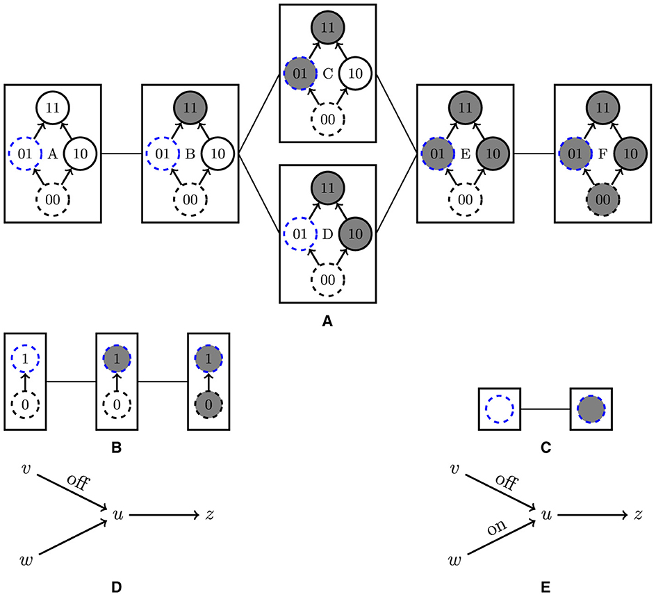
Figure 5. Embedding of factor graphs. (A) The u-factor graph for a node u with two sources and one target as pictured in (D, E). Each u-parameter is represented by a rectangle. Inside each rectangle is the Boolean lattice B^S(u) with each circle containing an input b = b_vb_w. Empty (filled) circles indicate inputs where the value of the logic parameter $f_u^1(b)=0$ ($f_u^1(b)=1$). The projection Φ(p; {v → u}, ∅) is determined by the values of $f_u^1$ on the dashed circles since ${\beta }^u={\beta }_v^u=0$ in the first component of the input. The projection Φ(p; {v → u}, {w → u}) is determined by the values on the blue circles, since ${\beta }^u={\beta }_v^u{\beta }_w^u=01$ based on the selection of OFF = {v → u},ON = {w → u}. The capital letters label each parameter for reference. (B) The u-factor graph after cutting the edge v → u. Using parameter D in (A) as the anchoring logic, setting OFF = {v → u} and ON = ∅, Ψ maps this factor graph isomorphically to the subgraph given by parameters D-E-F in (A). (C) The u-factor graph after cutting both v → u and w → u. Using parameter D in (a) as the anchoring logic, setting OFF = {v → u} and ON = {w → u}, Ψ maps this factor graph isomorphically to the subgraph D-E in (A). Using parameter B in (A) as the anchoring logic, Ψ maps this factor graph ismorphically to the subgraph B-C in (A). (D, E) The edges are labeled “off” or “on” according to the choice of OFF and ON in the descriptions of (B, C), respectively.

Our first result on Ψ is that the constraints on the set of anchoring logics $\mathcal{A}(N;\text{OFF},\text{ON})$ are sufficient for Ψ to be well defined. That is, we verify that any function f defined by Equations (20, 24) is a valid logic parameter.

Proposition 7.6. For any choice of anchoring logic $\widehat{f}\in \mathcal{A}(N;\text{OFF},\text{ON})$ and $q\in \mathcal{P}(C^{\overline{E}}(N))$, $\text{Ψ}(q;{\zeta }^{\text{OFF}},{\zeta }^{\text{ON}},\widehat{f})\in \mathcal{P}(N;{\zeta }^{\text{OFF}},{\zeta }^{\text{ON}},\widehat{f})$ so that Ψ is well defined.

Proof. Let q = (g, ϕ) and $(f,\theta )=\text{Ψ}(q;{\zeta }^{\text{OFF}},{\zeta }^{\text{ON}},\widehat{f})$. First, we show that $f_u^i$ is an MBF for each u and i. For $v\in \text{T}(u;\overline{E})$, the function $f_u^{{\theta }_u(v)}$ is constant and therefore trivially an MBF.

Let $v\in \text{T}(u;C^{\overline{E}}(N))$. Let b = (b¹, b²) and c = (c¹, c²) be elements of ${𝔹}^{\text{S}(u;C^{\overline{E}}(N))}\times {𝔹}^{\text{S}(u;\overline{E})}$ with b ≺ c.

• If b² = β^u = c² then b ≺ c implies b¹ ≺ c¹. Since $g_u^{{\varphi }_u(v)}$ is an MBF and f satisfies (Equation 20),

$f_u^{{\theta }_u(v)}(b^1,b^2)=g_u^{{\varphi }_u(v)}(b^1)\le g_u^{{\varphi }_u(v)}(c^1)=f_u^{{\theta }_u(v)}(c^1,c^2)$

• If both b² ≠ β^u and c² ≠ β^u then, since the anchoring logic ${\widehat{f}}_u^{{\theta }_u(v)}$ is an MBF and f satisfies (Equation 24),

$f_u^{{\theta }_u(v)}(b)={\widehat{f}}_u^{{\theta }_u(v)}(b)\le {\widehat{f}}_u^{{\theta }_u(v)}(c)=f_u^{{\theta }_u(v)}(c).$

• Let b² = β^u and c² ≠ β^u. Then b² ≺ c² implies β^u ≺ c² so that ${\widehat{f}}_u^{{\theta }_u(v)}(c^1,c^2)=1$. Therefore,

$f_u^{{\theta }_u(v)}(c^1,c^2)={\widehat{f}}_u^{{\theta }_u(v)}=1\ge f_u^{{\theta }_u(v)}(b^1,b^2).$

• Similarly, if b² ≠ β^u and c² = β^u, then b² ≺ c² implies b² ≺ β^u so that ${\widehat{f}}_u^{{\theta }_u(v)}(b^1,b^2)=0$. Therefore,

$f_u^{{\theta }_u(v)}(b^1,b^2)={\widehat{f}}_u^{{\theta }_u(v)}(b^1,b^2)=0\le f_u^{{\theta }_u(v)}(c^1,c^2).$

This shows that $f_u^i$ is an MBF.

Next, we show that f_u satisfies the ordering condition (Equation 1). Since the anchoring logic $\widehat{f}$ satisfies the ordering condition, when b² ≠ β^u

$f_u^i(b^1,b^2)={\widehat{f}}_u^i(b^1,b^2)\ge {\widehat{f}}_u^{i+1}(b^1,b^2)=f_u^{i+1}(b^1,b^2)$

and the ordering condition for f_u is satisfied. Suppose b² = β^u. Then

$f_u^i(b^1,b^2)=\{\begin{array}{ll}1,& \text{ if }i\le \left|\text{T}(u;\text{ON})\right|\\ 0,& \text{ if }i>\left|\text{T}(u;E\backslash \text{OFF})\right|\\ g_u^i(b^1),& \text{otherwise}.\end{array}$

Since g_u satisfies the ordering condition, this implies f_u satisfies the ordering condition at (b¹, b²).

It is straightforward to check that θ satisfies (Equation 19). Since we have shown that f is a valid logic parameter and f satisfies (Equation 24 by definition, $(f,\theta )\in \mathcal{P}(N;{\zeta }^{\text{OFF}},{\zeta }^{\text{ON}},\widehat{f})$.     □

We next establish that the collection of co-domains ${\left\{\mathcal{P}(N;{\zeta }^{\text{OFF}},{\zeta }^{\text{ON}},\widehat{f})\right\}}_{({\zeta }^{\text{OFF}},{\zeta }^{\text{ON}},\widehat{f})}$ of the collection of maps $\text{Ψ}(·;{\zeta }^{\text{OFF}},{\zeta }^{\text{ON}},\widehat{f})$, are disjoint. The fact that distinct choices of ζ^OFF or ζ^ON produce distinct sets of order parameters Θ(N; ζ^OFF, ζ^ON) follows directly from Equation 19.

Proposition 7.7. 1. The set of anchoring logics $\mathcal{A}(N;\text{OFF},\text{ON})$ is non-empty.

2. If $\widehat{f},ĥ\in \mathcal{A}(N;\text{OFF},\text{ON})$ are distinct anchoring logics then $\mathcal{P}(N;{\zeta }^{\text{OFF}},{\zeta }^{\text{ON}},\widehat{f})$ and $\mathcal{P}(N;{\zeta }^{\text{OFF}},{\zeta }^{\text{ON}},ĥ)$ are disjoint sets.

Proof. (1) It is straightforward to check that $\widehat{f}$ defined by

${\widehat{f}}_u^i(b^1,b^2)=\{\begin{array}{ll}0,& \text{ if }i>\left|\text{T}(u;E\backslash \text{OFF})\right|\text{ or }{b}^2\preccurlyeq {\beta }^u\\ 1,& \text{otherwise}\end{array}$

is a valid anchoring logic in $\mathcal{A}(N;\text{OFF},\text{ON})$.

(2) Suppose $\widehat{f}$ and ĥ are distinct anchoring logics. Then, there is a node u and index i such that the values of ${\widehat{f}}_u^i$ and ${ĥ}_u^i$ differ on an input (b¹, b²). Since $\widehat{f}$ and ĥ both satisfy (Equation 23), we must have that b² and β^u are incomparable, and hence b² ≠ β^u. Let $f\in \mathcal{P}(N;{\zeta }^{\text{OFF}},{\zeta }^{\text{ON}},\widehat{f})$ and $h\in \mathcal{P}(N;{\zeta }^{\text{OFF}},{\zeta }^{\text{ON}},ĥ)$. Since b² ≠ β^u and f and h satisfy (Equations 21, 26), we have $f_u^i(b^1,b^2)={\widehat{f}}_u^i(b^1,b^2)$ and $h_u^i(b^1,b^2)={ĥ}_u^i(b^1,b^2)$. This shows

$f_u^i(b^1,b^2)={\widehat{f}}_u^i(b^1,b^2)\ne {ĥ}_u^i(b^1,b^2)=h_u^i(b^1,b^2)$

so that f ≠ h. Since f and h are arbitrary, the statement holds.     □

We are now ready to prove Theorem 5.5 (3) which states that Ψ is a right inverse of Φ. It is implied immediately from the following theorem which also identifies $\mathcal{P}(N;{\zeta }^{\text{OFF}},{\zeta }^{\text{ON}},\widehat{f})$ as the image of Ψ.

Theorem 7.8. Fix ζ^OFF ∈ Θ(OFF), ζ^ON ∈ Θ(ON), and an anchoring logic $\widehat{f}\in \mathcal{A}(N;\text{OFF},\text{ON})$. The map $\text{Ψ}(·;{\zeta }^{\text{OFF}},{\zeta }^{\text{ON}},\widehat{f})$ is the inverse of Φ(·;OFF,ON) restricted to $\mathcal{P}(N;{\zeta }^{\text{OFF}},{\zeta }^{\text{ON}},\widehat{f})$.

Proof. First, we show that Ψ is a right inverse of Φ. Let $q=(g,\varphi )\in \mathcal{P}(C^{\overline{E}}(N))$ and $p=(f,\theta )=\text{Ψ}(q;{\zeta }^{\text{OFF}},{\zeta }^{\text{ON}},\widehat{f})$. We wish to show that Φ ∘ Ψ(q) = q.

Let $(\overline{g},\overline{\varphi })=\Phi (p;\text{OFF},\text{ON})$. First, we verify that $\overline{\varphi }=\varphi$. Let u ∈ V be a network node and $v\in \text{T}(u;C^{\overline{E}}(N))$. By Equation (25),

${\theta }_u(v)=\left|\text{T}(u;\text{ON})\right|+{\varphi }_u(v).$

By Equation (11) in the definition of Φ,

${\overline{\varphi }}_u(v)={\theta }_u(v)-{\#}_u(v).$

Since θ_u orders the edges in ON first and the edges in OFF last, for all w ∈ |T(u;ON)|, θ_u(w) < θ_u(v) and for all w ∈ T(u;OFF), θ_u(w) > θ_u(v). In particular, #_u(v) = |T(u;ON)| so that

${\overline{\varphi }}_u(v)=\left|\text{T}(u;\text{ON})\right|+{\varphi }_u(v)-{\#}_u(v)={\varphi }_u(v).$

This holds for each u and $v\in \text{T}(u;C^{\overline{E}}(N))$, that is, each node v in the domain of ϕ_u, so $\overline{\varphi }=\varphi$.

Next, we verify that $\overline{g}=g$. For a node u ∈ V, $v\in \text{T}(u;C^{\overline{E}}(N))$, and an input $b\in {𝔹}^{\text{S}(u;C^{\overline{E}}(N))}$

${\overline{g}}_u^{{\varphi }_u(v)}(b)=f_u^{{\theta }_u(v)}(b,{\beta }^u)=g_u^{{\varphi }_u(v)}(b)$

where the first equality follows from Equation (13) and the second equality follows from Equation (26). Since u and b were arbitrary, and $v\in \text{T}(u;C^{\overline{E}}(N))$ was an arbitrary target node of u in $C^{\overline{E}}(N)$, we must have $\overline{g}=g$.

Having shown Ψ is a right inverse, we now show that Ψ is a left inverse when Φ is restricted to $\mathcal{P}(N;{\zeta }^{\text{OFF}},{\zeta }^{\text{ON}},\widehat{f})$. Let $p=(f,\theta )\in \mathcal{P}(N;{\zeta }^{\text{OFF}},{\zeta }^{\text{ON}},\widehat{f})$, q = (g, ϕ) = Φ(p;OFF,ON), and $(\overline{f},\overline{\theta })=\text{Ψ}(q;{\zeta }^{\text{OFF}},{\zeta }^{\text{ON}},\widehat{f})$. We wish to show that Ψ ∘ Φ(p) = p.

First, we show that $\overline{\theta }=\theta$. For $v\in \text{T}(u;E\backslash \overline{E})$, we have

${\overline{\theta }}_u(v)=\left|\text{T}(u;\text{ON})\right|+{\varphi }_u(v)=\left|\text{T}(u;\text{ON})\right|+{\theta }_u(v)-{\#}_u(v)={\theta }_u(v)$

because #_u(v) = |T(u;ON)|. For v ∈ T(u;ON),

${\overline{\theta }}_u(v)={\zeta }_u^{\text{ON}}(v)={\theta }_u(v)$

because by definition of $\mathcal{P}(N;{\zeta }^{\text{ON}},{\zeta }^{\text{OFF}},\widehat{f})$ the order parameter θ satisfies (Equation 19) and therefore ${\theta }_u(v)={\zeta }_u^{\text{ON}}(v)$. Similarly, for v ∈ T(u;OFF),

${\overline{\theta }}_u(v)=\left|\text{T}(u;E\backslash \text{OFF})\right|+{\zeta }_u^{\text{OFF}}(v)={\theta }_u(v)$

because by definition θ orders the edges in OFF last and according to ζ^OFF. This covers all types of target nodes v of u. Since u was arbitrary, $\overline{\theta }=\theta$.

Next, we show that $\overline{f}=f$. For $v\in \text{T}(u;\overline{E})$, since $\overline{f}$ satisfies (Equation 24) and f satisfies (Equation 26), we have

${\overline{f}}_u^{{\theta }_u(v)}={\widehat{f}}_u^{{\theta }_u(v)}\equiv \{\begin{array}{ll}0,& \text{ if }v\in \text{T}(u;\text{OFF})\\ 1,& \text{ if }v\in \text{T}(u;\text{ON})\end{array}=f_u^{{\theta }_u(v)}.$

Now consider $v\in \text{T}(u;E\backslash \overline{E})$. Let $b^1\in {𝔹}^{\text{S}(u;C^{\overline{E}}(N))}$ and $b^2\in {𝔹}^{\text{S}(u;\overline{E})}$. For b² = β^u, we have

${\overline{f}}_u^{{\theta }_u(v)}(b^1,{\beta }^u)=g_u^{{\varphi }_u(v)}(b^1)=f_u^{{\theta }_u(v)}(b^1,{\beta }^u)$

where the first equality follows from Equation 26. For b² ≠ β^u, we have

${\overline{f}}_u^{{\theta }_u(v)}(b^1,b^2)={\widehat{f}}_u^{{\theta }_u(v)}(b^1,b^2)=f_u^{{\theta }_u(v)}(b^1,b^2)$

where the first equality follows from Equation 24, the definition of Ψ. The second equality follows from the definition of $\mathcal{P}(N;{\zeta }^{\text{OFF}},{\zeta }^{\text{ON}},\widehat{f})$. This completes the proof that $\overline{f}=f$.

Since $(\overline{f},\overline{\theta })=(f,\theta )$, we have that Ψ is a left inverse of the restricted Φ. Since Ψ is both a left and right inverse, Ψ is the inverse of the restricted Φ.     □

Finally, we prove Theorem 5.5 (4) which states that Ψ is a graph embedding of $\text{PG}(C^{\overline{E}}(N))$ into PG(N;OFF,ON).

Proof of Theorem 5.5 (4). Fix orderings ζ^OFF, ζ^ON, and anchoring logic $\widehat{f}\in \mathcal{A}(N;\text{OFF},\text{ON})$. We will show that $\text{Ψ}(·;{\zeta }^{\text{OFF}},{\zeta }^{\text{ON}},\widehat{f})$ maps $\text{PG}(C^{\overline{E}}(N))$ isomorphically into $\text{PG}(N;{\zeta }^{\text{OFF}},{\zeta }^{\text{ON}},\widehat{f})$. Since Theorem 7.8 shows that Ψ is invertible, it only remains to show that Ψ preserves parameter adjacency.

Let q = (g, ϕ) and $\overline{q}=(\overline{g},\overline{\varphi })$ be adjacent in $\text{PG}(C^{\overline{E}}(N))$. Let p = (f, θ) = Ψ(q) and $\overline{p}=\text{Ψ}(\overline{q})$. Let u be the unique node such that q_u and ${\overline{q}}_u$ are adjacent in the u-factor graph. Since Ψ is defined component-wise, for each w ≠ u, $p_w={\overline{p}}_w$.

To see that p_u and ${\overline{p}}_u$ are adjacent, first suppose q_u and ${\overline{q}}_u$ are order adjacent. Let π be the transposition of adjacent integers so that ${\varphi }_u=\pi \circ {\overline{\varphi }}_u$. Then, the adjacent transposition τ of {1, …, T(u; N)} is defined by

$\tau (i):=\{\begin{array}{ll}i,& \text{ if }i\le \left|\text{T}(u;\text{ON})\right|\\ \pi (i),& \text{ if }\left|\text{T}(u;\text{ON})\right|<i\le \left|\text{T}(u;E\backslash \text{OFF})\right|\\ i,& \text{ if }i>\left|\text{T}(u;E\backslash \text{OFF})\right|\end{array}$

satisfies ${\theta }_u=\tau \circ {\overline{\theta }}_u$. Moreover, since $g_u^i={\overline{g}}_u^{\tau (i)}$, it follows that $f_u^i={\overline{f}}_u^{\tau (i)}$. This shows that p_u and ${\overline{p}}_u$ are order adjacent.

Next, suppose q_u and ${\overline{q}}_u$ are logically adjacent. Since ${\varphi }_u={\overline{\varphi }}_u$ we have ${\theta }_u={\overline{\theta }}_u$. Let i be the unique index and $b\in {𝔹}^{\text{S}(u;C^{\overline{E}}(N))}$ be the unique input such that $g_u^i(b)\ne {\overline{g}}_u^i(b)$. Let $v={\varphi }_u^{-1}(i)$. Then, by Equation 26, we have

$f_u^{{\theta }_u(v)}(b,{\beta }^u)=g_u^i(b)\ne {\overline{g}}_u^i(b)={\overline{f}}_u^{{\theta }_u(v)}(b,{\beta }^u).$

On the other hand, for b¹ ≠ b, $g_u^i(b^1)={\overline{g}}_u^i(b^1)$ because g and $\overline{g}$ are adjacent logic parameters in $\mathcal{L}(C^{\overline{E}}(N))$. Therefore,

$f_u^{{\theta }_u(v)}(b^1,{\beta }^u)=g_u^i(b^1)={\overline{g}}_u^i(b^1)={\overline{f}}_u^{{\theta }_u(v)}(b^1,{\beta }^u).$

On the input (b¹, b² ≠ β^u), the value of f_u and ${\overline{f}}_u$ is determined by the reference logic $\widehat{f}$ and thus they agree:

$f_u^{{\theta }_u(v)}(b^1,b^2)={\widehat{f}}_u^{{\theta }_u(v)}(b^1,b^2)={\overline{f}}_u^{{\theta }_u(v)}(b^1,b^2).$

That is, (b, β^u) is the unique input so that $f_u^{{\theta }_u(v)}(b,{\beta }^u)\ne {\overline{f}}_u^{{\theta }_u(v)}(b,{\beta }^u)$.

Next we show that for w ∈ T(u; N)\{v}, $f_u^w={\overline{f}}_u^w$. If $w\in \text{T}(u;E\backslash \overline{E})$ then $g_u^{{\varphi }_u(w)}={\overline{g}}_u^{{\varphi }_u(w)}$ because g_u and ${\overline{g}}_u$ differ only at component i = ϕ_u(v). Therefore for such a w

$f_u^{{\theta }_u(w)}(b^1,{\beta }^u)=g_u^{{\varphi }_u(w)}(b^1)={\overline{g}}_u^{{\varphi }_u(w)}(b^1)={\overline{f}}_u^{{\theta }_u(w)}(b^1,{\beta }^u)$

and for $b^2\ne {\beta }_u$,

$f_u^{{\theta }_u(w)}(b^1,b^2)={\widehat{f}}_u^{{\theta }_u(w)}(b^1,b^2)={\overline{f}}_u^{{\theta }_u(w)}(b^1,b^2).$

On the other hand, if $w\in \text{T}(u;\overline{E})$ then

$f_u^{{\theta }_u(w)}\equiv \{\begin{array}{ll}0,& \text{ if }w\in \text{T}(u;\text{OFF})\\ 1,& \text{ if }w\in \text{T}(u;\text{ON})\end{array}\equiv {\overline{f}}_u^{{\theta }_u(w)}.$

We conclude that θ_u(v) is the unique index such that $f_u^{{\theta }_u(v)}\ne {\overline{f}}_u^{{\theta }_u(v)}$. That is, p_u and ${\overline{p}}_u$ are logically adjacent.

Since Ψ is invertible and adjacency of q and $\overline{q}$ implies adjacency of p and $\overline{p}$, we conclude Ψ is an isomorphism.     □

8 Algebraic properties of the projection maps

Theorem 8.1. (a) Let $\overline{E}={\overline{E}}_1\bigsqcup {\overline{E}}_2\subset E$, where ${\overline{E}}_1=\text{ON}$ and ${\overline{E}}_2=\text{OFF}$. The V-dual parameter map D^V commutes with the projection map Φ(·;OFF,ON) when the identities of OFF and ON edges are exchanged:

$D^V\circ \Phi (·;{\overline{E}}_1,{\overline{E}}_2)=\Phi (·;{\overline{E}}_2,{\overline{E}}_1)\circ D^V.$

(b) Let $\overline{E}=\left\{e\right\}$. The V-dual parameter map D^V commutes with the projection map Φⁱⁿ(·;e):

$D^V\circ {\Phi }^{in}(·;e)={\Phi }^{in}(·;e\circ D^V.$

Proof. (a) Let $p=(f,\theta )\in \mathcal{P}(N)$. Let

$q=(g,\varphi )=D^V(\Phi (p;{\overline{E}}_1,{\overline{E}}_2))\text{ and }\overline{q}=(\overline{g},\overline{\varphi })=\Phi (D^V(p);{\overline{E}}_2,{\overline{E}}_1).$

We will show that $q=\overline{q}$.

First, we show that $\varphi =\overline{\varphi }$. Recall (see Equation 10) that we defined the number of out-edges of u with rank less than θ_u(v)

${\#}_u(v;p,\overline{E})=\left|\left\{i<{\theta }_u(v)|{\theta }_u^{-1}(i)\in \text{T}(u;\overline{E})\right\}\right|$

where we now explicitly include the dependency on the parameter p = (f, θ). From Equation 4, 11, for each $u⊸v\in E\backslash \overline{E}$ we have

$\begin{array}{l}{\varphi }_u(v)=\left|\text{T}(u;C^{\overline{E}}(N))\right|+1-({\theta }_u(v)-{\#}_u(v;p)),\text{ and }\\ {\overline{\varphi }}_u(v)=(\left|\text{T}(u;N)\right|+1-{\theta }_u(v))-{\#}_u(v;D^V(p)).\end{array}$

We therefore need to show that

$\begin{array}{c}\left|\text{T}(u;C^{\overline{E}}(N))\right|+{\#}_u(v;p)=\left|\text{T}(u;N)\right|-{\#}_u(v;D^V(p)),\text{ or }\\ {\#}_u(v;D^V(p))=\left|\text{T}(u;N)\right|-\left|\text{T}(u;C^{\overline{E}}(N))\right|-{\#}_u(v;p).\end{array}$

Note that $\left|\text{T}(u;N)\right|-\left|\text{T}(u;C^{\overline{E}}(N))\right|=\left|\text{T}(u;\overline{E})\right|$ is the number of cut edges which have source u. To compute ${\#}_u(v;D^V(p))$, let $\overline{\theta }$ be the order parameter for D^V(p) and m_u = |T(u; N)|. We have

$\begin{array}{l}{\#}_u(v;D^V(p))=\left|\left\{i<{\overline{\theta }}_u(v)|{\overline{\theta }}_u^{-1}(i)\in |\text{T}(u;\overline{E})|\right\}\right|\\ =\left|\left\{m_u+1-i<{\overline{\theta }}_u(v)|{\overline{\theta }}_u^{-1}(m_u+1-i)\in |\text{T}(u;\overline{E})|\right\}\right|\\ =\left|\left\{i\ge {\theta }_u(v)|{\theta }_u^{-1}(i)\in |\text{T}(u;\overline{E})|\right\}\right|\\ =\left|\text{T}(u;\overline{E})\right|-{\#}_u(v;p),\end{array}$

as desired.

Now we show $g=\overline{g}$. Let $(\tilde{g},\tilde{\varphi })=\Phi (p;{\overline{E}}_1,{\overline{E}}_2)$. By Equation 13, for each $u⊸v\in E\backslash \overline{E}$

${\tilde{g}}_u^{{\tilde{\varphi }}_u(v)}(b)=f_u^{{\theta }_u(v)}(b,{\beta }^u({\overline{E}}_1,{\overline{E}}_2).$

Since $(g,\varphi )=D^V((\tilde{g},\tilde{\varphi }))$,

$\begin{array}{cc}{g}_u^{{\varphi }_u(v)}(b)=\neg {\tilde{g}}_u^{{\tilde{\varphi }}_u(v)}(\neg b)=\neg f_u^{{\theta }_u(v)}(\neg b,{\beta }^u({\overline{E}}_1,{\overline{E}}_2))& (27)\end{array}$

where in the first equality, we have used ${\overline{\varphi }}_u(v)=\left|\text{T}(u;C^{\overline{E}}(N))\right|+1-{\varphi }_u(v)$. Let $(\tilde{f},\tilde{\theta })=D^V((f,\theta ))$. By Equation 4,

${\tilde{f}}_u^{{\tilde{\theta }}_u(v)}(b^1,b^2)=\neg f_u^{{\theta }_u(v)}(\neg b^1,\neg b^2).$

Since $(\overline{g},\overline{\varphi })=\Phi ((\tilde{f},\tilde{\theta }),{\overline{E}}_2,{\overline{E}}_1)$, we have

$\begin{array}{cc}{\overline{g}}_u^{{\overline{\varphi }}_u(v)}(b)={\tilde{f}}_u^{{\tilde{\theta }}_u(v)}(b,{\beta }^u({\overline{E}}_2,{\overline{E}}_1))=\neg f_u^{{\theta }_u(v)}(\neg b,\neg {\beta }^u({\overline{E}}_2,{\overline{E}}_1)).& (28)\end{array}$

We have already shown that $\overline{\varphi }=\varphi$. By inspecting the definition of β^u in Equation 12, it is also clear that ${\beta }^u({\overline{E}}_1,{\overline{E}}_2)=\neg {\beta }^u({\overline{E}}_2,{\overline{E}}_1)$. Comparing the expressions for g in Equation 27 and $\overline{g}$ in Equation 28, we conclude that $g=\overline{g}$. This proves first part of the Theorem.

To prove the second part, we note that the only difference between Φ and Φⁱⁿ is that in the definition of logic parameter g, the input from the cut edge e is replaced by arbitrary value β, rather than a specific value that depend on whether the cut edge belongs to ON and OFF. Therefore, this construction proves also the second statement.     □

Since the projection map Φ and the V-dual parameter map commute, it is natural to expect that the corresponding maps between STGs, ρ^OFF,ON, ${\mu }^{\overline{E}}$, and λ^V commute as well. In the following two propositions, we show that this is indeed the case.

The first proposition relates attractors $X({\overline{E}}_1,{\overline{E}}_2)$ (see 7.1) in the STG of the full network N and the STG of the cut network $X(C^{\overline{E}}(N))$ under the map λ^V.

Proposition 8.2. Let $\overline{E}={\overline{E}}_1\bigsqcup {\overline{E}}_2\subset E$. The following diagram commutes

Proof. First, we prove that image of $X({\overline{E}}_1,{\overline{E}}_2)$ under λ^V(·;N) is $X({\overline{E}}_2,{\overline{E}}_1)$. Let $x\in X({\overline{E}}_1,{\overline{E}}_2)$. For each node u ∈ V, $x_u\in X_u({\overline{E}}_1,{\overline{E}}_2)$ implies

$\left|\text{T}(u;{\overline{E}}_2)\right|\le x_u\le \left|\text{T}(u;N)\right|-\left|\text{T}(u;{\overline{E}}_1)\right|.$

Since ${\lambda }_u^V(x_u;N)=\left|\text{T}(u;N)\right|-x_u$,

$\left|\text{T}(u;{\overline{E}}_1)\right|\le x_u\le \left|\text{T}(u;N)\right|-\left|\text{T}(u;{\overline{E}}_2)\right|$

and therefore $x_u\in X_u({\overline{E}}_2,{\overline{E}}_1)$. This holds for each u which implies ${\lambda }^V(x;N)\in X({\overline{E}}_2,{\overline{E}}_1)$.

Next, we show

$\begin{array}{cc}{\rho }^{{\overline{E}}_1,{\overline{E}}_2}={\lambda }^V(·;C^{\overline{E}}(N))\circ {\rho }^{{\overline{E}}_2,{\overline{E}}_1}\circ {\lambda }^V(·;N).& (29)\end{array}$

Since λ^V is an involution and ρ is invertible, this will prove the proposition. Let $x\in X({\overline{E}}_1,{\overline{E}}_2)$ and u ∈ V. We have

${\rho }_u^{{\overline{E}}_1,{\overline{E}}_2}(x_u)=x_u-\left|\text{T}(u;{\overline{E}}_2)\right|.$

On the other hand,

$\begin{array}{l}\left[{\lambda }_u^V(·;C^{\overline{E}}(N))\circ {\rho }_u^{{\overline{E}}_2,{\overline{E}}_1}\circ \lambda (·;N)\right](x_u)\\ =\left[{\lambda }_u^V(·;C^{\overline{E}}(N))\circ {\rho }_u^{{\overline{E}}_2,{\overline{E}}_1}\right](\left|\text{T}(u;N)\right|-x_u)\\ =\left[{\lambda }_u^V(·;C^{\overline{E}}(N))\right](\left|\text{T}(u;N)\right|-x_u-\left|\text{T}(u;{\overline{E}}_1)\right|)\\ =\left|\text{T}(u;E\backslash \overline{E})\right|-(\left|\text{T}(u;N)\right|-x_u-\left|\text{T}(u;{\overline{E}}_1)\right|)\\ =x_u+\left|\text{T}(u;E\backslash \overline{E})\right|-\left|\text{T}(u;N)\right|+\left|\text{T}(u;{\overline{E}}_1)\right|\\ =x_u-(\left|\text{T}(u;\overline{E})\right|-\left|\text{T}(u;{\overline{E}}_1)\right|)\\ =x_u-\left|\text{T}(u;{\overline{E}}_2)\right|.\end{array}$

Since u was arbitrary, the statement (Equation 29) holds, which finishes the proof of the proposition.

     □

The second proposition relates the surjective map μ^e(N), used in relating state transition graphs for input inessential parameters in Theorem 5.4, and the map λ^V.

Proposition 8.3. Let $p=(f,\theta )\in \mathcal{P}(N)$ and (f′, θ′) = D^V(p) be the V-dual parameter of p. Let e = u ⊸ v be an edge. The following diagram commutes

Proof. We will prove

${\mu }^e(·;\theta )={\lambda }^V(·;C^e(N))\circ {\mu }^e(·;{\theta }^{\prime })\circ {\lambda }^V(·;N).$

Since λ^V is an involution, this will prove the proposition.

Let M = C^e(N). For w ≠ u, ${\mu }_w^e$ is the identity. Furthermore, ${\lambda }_w^V(·;M)={\lambda }_w^V(·;N)$ since X_w(M) = X_w(N). Since ${\lambda }_w^V$ is its own inverse, this shows

${\mu }_w^e(·;\theta )={\lambda }_w^V(·;M)\circ {\mu }_w^e(·;{\theta }^{\prime })\circ {\lambda }_w^V(·;N).$

Now consider the u component and let x ∈ X. We have

$\begin{array}{l}({\lambda }_u^V(·;M)\circ {\mu }_u^e(·;{\theta }^{\prime })\circ {\lambda }_u^V(·;N))(x_u)\\ =|\text{T}(u;M)|-{\mu }_u^e(|\text{T}(u;N)|-x_u;{\theta }^{\prime })\\ =|\text{T}(u;M)|-\{\begin{array}{ll}|\text{T}(u;N)|-x_u\hfill & \text{ if }|\text{T}(u;N)|-x_u<{\theta }_{u^{\prime }}(v)\hfill \\ |\text{T}(u;N)|-x_u-1\hfill & \text{ if }|\text{T}(u;N)|-x_u\ge {\theta }_{u^{\prime }}(v)\hfill \end{array}\\ =\{\begin{array}{ll}{x}_u-1\hfill & \text{ if }{x}_u\ge {\theta }_u(v)\hfill \\ x_u\hfill & \text{ if }{x}_u<{\theta }_u(v)\hfill \end{array}={\mu }_u^e(x_u)\end{array}$

where the last line follows from

$\left|\text{T}(u;M)\right|=\left|\text{T}(u;N)\right|-1\text{ and }{\theta }_u(v)=\left|\text{T}(u;N)\right|+1-{\theta }_u^{\prime }(v).$

     □

Finally, we prove that projections commute and that successive projections are equivalent to projecting every edge simultaneously.

Proposition 8.4. The projection map Φ satisfies the following properties.

1. Φ(·;∅, {e₂}) ∘ Φ(·;{e₁}, ∅) = Φ(·;{e₁}, {e₂}) = Φ(·;{e₁}, ∅) ∘ Φ(·;∅, {e₂}).

2. Φ(·;{e₁}, ∅) ∘ Φ(·;{e₂}, ∅) = Φ(·;{e₁, e₂}, ∅) = Φ(·;{e₂}, ∅) ∘ Φ(·;{e₁}, ∅).

3. Φ(·;∅, {e₁}) ∘ Φ(·;∅, {e₂}) = Φ(·;∅, {e₁, e₂}) = Φ(·;∅, {e₂}) ∘ Φ(·;∅, {e₁}).

The projection map Φⁱⁿ satisfies

$(4){\Phi }^{in}(·;e_1)\circ {\Phi }^{in}(·;e_2)={\Phi }^{in}(·;\left\{e_1,e_2\right\})={\Phi }^{in}(·;e_2)\circ {\Phi }^{in}(·;e_1).$

Finally,

$\begin{array}{cc}(5)& {\Phi }^{in}(·;e_1)\circ \Phi (·;\varnothing ,\left\{e_2\right\})=\Phi (·;\varnothing ,\left\{e_2\right\})\circ {\Phi }^{in}(·;e_1)\\ (6)& {\Phi }^{in}(·;e_1)\circ \Phi (·;\left\{e_2\right\},\varnothing ,)=\Phi (·;\left\{e_2\right\},\varnothing )\circ {\Phi }^{in}(·;e_1)\end{array}$

Proof. (1): We first show that

$\Phi (·;\varnothing ,\left\{e_2\right\})\circ \Phi (·;\left\{e_1\right\},\varnothing )=\Phi (·;\left\{e_1\right\},\left\{e_2\right\}).$

Let $p=(f,\theta )\in \mathcal{P}(N)$, q = (g, ϕ) = Φ(p; {e₁}, {e₂}), and

$\overline{q}=(\overline{g},\overline{\varphi })=\Phi (·;\varnothing ,\left\{e_2\right\})\circ \Phi (·;\left\{e_1\right\},\varnothing )(p).$

We will show that $q=\overline{q}$.

First, we show that $\varphi =\overline{\varphi }$. Recall from Equation 10 that

${\#}_u(v;p,\overline{E})=\left|\left\{i<{\theta }_u(v)|{\theta }_u^{-1}(i)\in \text{T}(u;\overline{E})\right\}\right|$

where we now explicitly include the dependencies on the parameter p = (f, θ) and the edges $\overline{E}$. Let $\tilde{p}=(\tilde{f},\tilde{\theta })=\Phi (p;\left\{e_1\right\},\varnothing )$. By Equation 11,

$\begin{array}{l}{\varphi }_u(v)={\theta }_u(v)-{\#}_u(v;p,\left\{e_1,e_2\right\})\\ {\overline{\varphi }}_u(v)={\theta }_u(v)-{\#}_u(v;p,\left\{e_1\right\})-{\#}_u(v;\tilde{p},\left\{e_2\right\}).\end{array}$

To prove $\varphi =\overline{\varphi }$, we need to show that

${\#}_u(v;p,\left\{e_1,e_2\right\})={\#}_u(v;p,\left\{e_1\right\})+{\#}_u(v;\tilde{p},\left\{e_2\right\}).$

Applying Equation 11 to $\tilde{\theta }$ and using the definition of #_u, we have

$\begin{array}{l}{\#}_u(v;\tilde{p},\{e_2\})=\left|\text{{}i<{\tilde{\theta }}_u(v)\text{ | }{\tilde{\theta }}_u^{-1}(i)\in \text{T}(u;\{e_2\})\}\right|\\ =\left|\text{{}i<{\theta }_u(v)-{\#}_u(v;p,\{e_1\})\text{ | }{\theta }_u^{-1}(i+{\#}_u(v;p,\left\{e_1\right\})\in \text{T}(u;\left\{e_2\right\})\}\right|\\ =\left|\text{{}i<{\theta }_u(v)\text{ | }{\theta }_u^{-1}(i)\in \text{T}(u;\{e_2\})\text{ }}\right|={\#}_u(v;p,\{e_2\}).\end{array}$

Since ${\#}_u(v;p,\overline{E})$ counts the number of edges θ_u below u ⊸ v, we have

${\#}_u(v;p,\left\{e_1\right\})+{\#}_u(v;p,\left\{e_2\right\})={\#}_u(v;p,\left\{e_1,e_2\right\}).$

We therefore conclude $\varphi =\overline{\varphi }$.

Next, we show that $g=\overline{g}$. Applying Equation 13,

$\begin{array}{l}{g}_u^{{\varphi }_u(v)}(b)=f_u^{{\theta }_u(v)}(b,{\beta }^u(\left\{e_1\right\},\left\{e_2\right\})),\text{ and }\\ {\overline{g}}^{{\overline{\varphi }}_u(v)}(b)={\tilde{f}}_u^{{\tilde{\theta }}_u(v)}(b,{\beta }^u(\varnothing ,\left\{e_2\right\}))=f_u^{{\theta }_u(v)}(b,{\beta }^u(\varnothing ,\left\{e_2\right\}),{\beta }^u(\left\{e_1\right\},\varnothing )).\end{array}$

Since we have shown $\varphi =\overline{\varphi }$ and ${\beta }^u(\left\{e_1\right\},\left\{e_2\right\})=({\beta }^u(\varnothing ,\left\{e_2\right\}),{\beta }^u(\left\{e_1\right\},\varnothing ))$ is clear from the definition of β, $g=\overline{g}$. This completes the proof of the first equality in (1).

To show the second equality, we apply Theorem 8.1 and the fact that D^V is an involution to the first equality:

$\begin{array}{l}\Phi (·;\left\{e_1\right\},\left\{e_2\right\})=D^V\circ \Phi (·;\left\{e_2\right\},\left\{e_1\right\})\circ D^V\\ =D^V\circ \Phi (·;\varnothing ,\left\{e_1\right\})\circ \Phi (·;\left\{e_2\right\},\varnothing )\circ D^V\\ =\Phi (·;\left\{e_1\right\},\varnothing )\circ D^V\circ D^V\circ \Phi (·;\varnothing ,\left\{e_2\right\})\\ =\Phi (·;\left\{e_1\right\},\varnothing )\circ \Phi (·;\varnothing ,\left\{e_2\right\}).\end{array}$

Both equalities in (2) follow from a similar argument for the first equality in (1). Statement (3) follows from applying Theorem 8.1 to (2). Statement (4) follows from statement (3) and a realization that the only difference between Φ and Φⁱⁿ is independence of the latter on division of cut edges into ON and OFF. Similar argument implies that statements (5) and (6) follow from (1) and (2).

     □

9 Network example

We describe the embeddings of the parameter graph of negative feedback loop PG(NL) and parameter graph of the positive loop PG(PL) into parameter graph PG(N) of the network N in Figure 1A. Theorem 5.5 requires that the edges that are cut from N to arrive at a subgraph NL, or PL, are output inessential.

We first consider the negative loop which requires that we cut the edge e: = z → y from N and therefore $\overline{E}=\left\{e\right\}$. There are two choices for edge e to be output inessential: this edge can be always ON and thus output-on inessential, or always OFF, and hence output-off inessential. Cutting this edge produces network C^e(N) = NL which consists of negative loop z → x ⊣ y → z. Since each node in this loop has one input edge and one output edge, the parameter graph PG(NL) is a product of three copies of factor graph PG(x) with 27 elements

$\text{PG}(NL)=\text{PG}(x)\times \text{PG}(x)\times \text{PG}(x).$

There are two embeddings: If e is output-on inessential there is an embedding ${\text{Ψ}}_1:\text{PG}(NL)\to \mathcal{P}(N;\varnothing ,\left\{e\right\})\subset \text{PG}(N)$, and when e is output-off inessential, there is an ${\text{Ψ}}_2:\text{PG}(NL)\to \mathcal{P}(N;\left\{e\right\},\varnothing )\subset \text{PG}(N)$. These are illustrated in Figure 1 and further explained below.

Checking the Table 3, the edge e is always ON in parameters that 7, 8, and 10 while always OFF in parameters 3, 5, and 6. Looking now at Table 2, the input from z being ON corresponds to first and third rows of the truth table, where the input from x determines the value of the MBF. The nodes I, II, and IV parameterize possible behaviors of the input edge x ⊣ y. Similarly, considering Table 2, input z being OFF corresponds to second and fourth rows of the truth table. In this case, the nodes IV, V, and VI parameterize possible behaviors of the input edge x ⊣ y.

Therefore, the embedding Ψ₁(PG(NL)) is

$(u,v,w)\in \left\{A,B,C\right\}\times \left\{\text{I,II,IV}\right\}\times \left\{7,8,10\right\}.$

The embedding Ψ₂(PG(NL)) is

$(u,v,w)\in \left\{A,B,C\right\}\times \left\{\text{IV,V,VI}\right\}\times \left\{3,5,6\right\},$

Note that the fact that these embeddings intersect does not contradict Theorem 7.7, since both of these embeddings have a single anchor logic.

We also note that the oscillatory behavior in the PG(NL) is supported by its central node. This node embeds into

$\begin{array}{cc}(B,II,5)\text{ and }(B,V,8)\text{ by }{\text{Ψ}}_1\text{ and }{\text{Ψ}}_2,\text{ respectively}.& (30)\end{array}$

We conclude that these two nodes in PG(N) support oscillatory behavior.

The embedding of PG(PL) into PG(N) requires that the edges e_yx:x ⊣ y and e_xz:z → x are output inessential. The first condition corresponds to node A, when x ⊣ y is output-off inessential, and to node C when x ⊣ y is output-on inessential. The edge z → x is output-on inessential at nodes 1, 2, and 3 and output-off inessential at nodes 10, 11, and 12. Therefore, there are four embeddings given by combinations of labels ON and OFF on edges e_yx, e_xz. Evaluating the MBF at node y in Table 2 on the appropriate constant input from x as above, we obtain disjoint embeddings of PG(PL) into PG(N):

$\begin{array}{l}(ON,ON):(u,v,w)\in \left\{C\right\}\times \{\text{III},\text{V},\text{ VI}\}\times \{1,2,3\}\\ (ON,OFF):(u,v,w)\in \left\{C\right\}\times \{\text{III},\text{V},\text{VI}\}\times \{10,11,12\}\\ (OFF,ON):(u,v,w)\in \left\{A\right\}\times \{\text{I},\text{II},\text{III}\}\times \{1,2,3\}\\ (OFF,OFF):(u,v,w)\in \left\{A\right\}\times \{\text{I},\text{II},\text{II}\}\times \{10,11,12\}\end{array}$

We note that the bistable behavior in the PG(PL) is only supported by its central node. This node embeds into

$(C,\text{V},2),(C,\text{V},11),(A,\text{II},2),\text{ and }(A,\text{II},11)\text{ respectively.}$

We conclude that these four nodes in PG(N) support bistable behavior.

So far, we only considered cutting of output inessential edges which results in the embedding of the entire parameter graph. We now consider parameters at which the edges that are being cut are input inessential.

9.1 Input inessential parameters

We now describe input inessential parameters (u, v, w) ∈ PG(x) × PG(y) × PG(z) (see Figure 1) which support the dynamics of the negative loop NL. Such parameters must satisfy two properties:

1. support essential edges forming the negative feedback loop NL; and

2. the edge z → y must be input inessential at y.

To satisfy the first condition, the only choice in PG(x) is B since choices A and C would disconnect the loop at the network node x. In PG(y), the only option is node III where the edge z → y is input essential. At node z to satisfy the first condition, we can choose from nodes 4, 5, 8, and 9. Apart from essential nodes 4 and 9, at parameter nodes 5 and 8 the edge z → x that participates in the negative loop is output essential.

Therefore at 4 parameters

$(B,\text{III},w)\text{ where }w\in \left\{4,5,8,9\right\}$

Theorem 5.4 applies. There is a semi-conjugacy of the dynamics on the state transition graph, and therefore, these parameters support oscillations generated by the negative feedback loop.

Similar arguments show that all parameters where at least one of the edges e_yx and e_xz is input inessential, but the bistable loop is essential, will exhibit bistable dynamics.

We first consider the first condition that e_yx is input inessential. This does not affect the choice of parameter in PG(x), so all three nodes are acceptable. In PG(y), the only MBF where e_yx is input inessential, e_yz is input essential, and where the edge e_zy is output essential is the function IV. In PG(z), the nodes where the edge e_yz is output essential are {2, 4, 9, 11}. Therefore for parameter combinations

$\begin{array}{cc}(u,v,w)\in \text{PG}(N),\text{ with }u\in \left\{A,B,C\right\},v\in \left\{\text{IV}\right\},w\in \left\{2,4,9,11\right\}& (31)\end{array}$

there is a semi-conjugacy of state transition graph dynamics onto dynamics of positive loop PL, which exhibits bistability.

The second condition that e_xz is input inessential is satisfied in PG(x) by functions A and C. At PG(y), three choices II, IV,V make e_yz input essential, while choices {2, 4, 9, 11} in PG(z) make the edge e_yz output essential. Therefore for parameters

$\begin{array}{cc}(u,v,w)\in \text{PG}(N),\text{ with }u\in \left\{A,C\right\},v\in \left\{\text{II,IV,V}\right\},w\in \left\{2,4,9,11\right\}& (32)\end{array}$

Theorem 5.4 also implies existence of bistability. Both edges e_yx and e_xz are input in-essential on parameters where two collections (Equation 31) and (Equation 32) overlap.

It is now possible to investigate relative positions of parameters that support bistability and those that support oscillations. For instance, parameter (B, II, 5) supports oscillation (see Equation 30) and parameter (C, II, 4) supports bistability (see Equation 32). These parameters are not neighbors in the parameter space, but a simultaneous lowering of activation threshold of x ⊣ y and lowering of activation threshold of z → y, changes the dynamic behavior of the network N.

10 Discussion

In this article, we study a question of the relationship between network structure and its dynamics. In the DSGRN approach, the parameter space of switching ODE systems compatible with the network structure is first decomposed into a finite number of domains that correspond to multi-level Boolean systems [7] and then organized into a finite parameter graph. This supports a description of the dynamics by finite state transition graphs and allows us to formulate our question precisely. Because the finitness of this description avoids algorithmically difficult questions of existence of smooth conjugacies, this framework provides a tractable way to address this question. The price we pay is that the description of the dynamics is by necessity approximate and only captures features of the dynamics that are stable under parameter perturbations.

DSGRN analysis is in some sense complementary to the analysis of equations of mass action kinetics. Enzymatic chemical reactions in cellular biology are often modeled by saturating Hill functions. While DSGRN follows a switching system approximation of Hill functions by piecewise constant functions, thus emphasizing the saturating behavior of the Hill functions, the mass action polynomial approximation emphasizes the non-saturated part of the Hill function. General lack of experimentally determined values of parameters requires the development of combinatorial, often graph based, approaches for both types of approximations [55–58].

The main result of the study describes how dynamics of a subnetwork manifests itself in the dynamics of a larger network. In systems biology, the concept of a network is central to understanding the function of a cell and its responses to the environment. Unfortunately, the networks studied by biologists are always incomplete, uncertain, and the parameters mostly unmeasurable. Yet the need for predictive models is very high. The results presented here suggest that the DSGRN approach can provide precise understanding of whether or not a network can produce distinct phenotypes (i.e., normal vs. cancer) and how robust are such predictions under network embedding, provided that the expectations imposed on predictive modeling are properly adjusted, that is, there is no expectation that our approach can reproduce precise time series trajectories of multiple genes.

A popular link between structure and function has been proposed in the theory of motifs [39–41]. In this approach, a search over large databases of regulatory networks revealed statistically significant over-representation of certain 3-4 node subnetworks, called motifs. The hypothesis, supported by simple models and a compelling narrative, is that these motifs are over-represented because they serve a particular cellular function. However, there is limited evidence that these small subnetworks consistently work in the same way within the larger networks as they do in isolation.

Our present study provides some answer to these questions. We show that the dynamics of the subnetwork can be always found in the dynamics of the larger network, provided that it is “uncovered” by setting parameters of the additional edges of the larger network to be constitutively ON or OFF. As such, the larger network is always capable of reproducing dynamics of each of its subnetworks for an appropriate choice of parameters.

Another important conjecture in systems biology asserts that the reason why we observe large networks exhibiting dynamics that smaller networks can produce on their own (say oscillations) is that redundancy enhances robustness of the phenotype. Our observation that the parameter graph PG(M) of the subnetwork M is embedded in multiple copies in the parameter graph PG(N) of network N supports this assertion. We did not directly study the mutual position of these embedded subgraphs within the larger graph beyond showing they are disjoint. The robustness argument would be strengthened if these subgraphs lie close to each other in such a way that perturbation of a node in one may lead to a node in the other embedding with the same dynamics.

We believe that the proposed framework of DSGRN to study the relationship between network structure and its function (i.e., dynamics) will provide many important insights in systems biology.

Data availability statement

The original contributions presented in the study are included in the article, further inquiries can be directed to the corresponding author.

Author contributions

WD: Writing – original draft, Visualization, Investigation, Formal analysis. BC: Writing – review & editing. TG: Writing – review & editing, Supervision, Conceptualization.

Funding

The author(s) declare financial support was received for the research, authorship, and/or publication of this article. This research was partially supported by NIH 5R01GM126555-01.

Conflict of interest

WD was employed by Immunetrics.

The remaining authors declare that the research was conducted in the absence of any commercial or financial relationships that could be construed as a potential conflict of interest.

The author(s) declared that they were an editorial board member of Frontiers, at the time of submission. This had no impact on the peer review process and the final decision.

Publisher's note

All claims expressed in this article are solely those of the authors and do not necessarily represent those of their affiliated organizations, or those of the publisher, the editors and the reviewers. Any product that may be evaluated in this article, or claim that may be made by its manufacturer, is not guaranteed or endorsed by the publisher.

References

1. Katok A, Hasselblatt B. Introduction to Modern Theory of Dynamical Systems. Cambridge: Cambridge University Press. (1995). doi: 10.1017/CBO9780511809187

Crossref Full Text | Google Scholar

2. Newhouse S. The abundance of wild hyperbolic sets and non-smooth stable sets for diffeomorphisms. Publ Math IHES. (1979) 50:101–51. doi: 10.1007/BF02684771

Crossref Full Text | Google Scholar

3. Cummins B, Gedeon T, Harker S, Mischaikow K, Mok K. Combinatorial representation of parameter space for switching systems. SIAM J Appl Dyn Syst. (2016) 15:2176–212. doi: 10.1137/15M1052743

PubMed Abstract | Crossref Full Text | Google Scholar

4. Cummins B, Gedeon T, Harker S, Mischaikow K. Database of dynamic signatures generated by regulatory networks (DSGRN). In: Koeppl JFH, , editor. Computational Methods in Systems Biology - 2017. Cham: Springer (2017). p. 300–308. doi: 10.1007/978-3-319-67471-1_19

Crossref Full Text | Google Scholar

5. Gedeon T, Cummins B, Harker S, Mischaikow K. Identifying robust hysteresis in networks. PLoS Comput Bio. (2018) 14:e1006121. doi: 10.1371/journal.pcbi.1006121

PubMed Abstract | Crossref Full Text | Google Scholar

6. Gedeon T. Multi-parameter exploration of dynamics of regulatory networks. Biosystems. (2020) 190:104113. doi: 10.1016/j.biosystems.2020.104113

PubMed Abstract | Crossref Full Text | Google Scholar

7. Crawford-Kahrl P, Cummins B, Gedeon T. Joint realizability of monotone boolean functions. J Theor Comp Sci. (2022) 922:447–74. doi: 10.1016/j.tcs.2022.04.045

PubMed Abstract | Crossref Full Text | Google Scholar

8. Glass L, Kauffman S. Co-operative components, spatial localization and oscillatory cellular dynamics. J Theoret Biol. (1972) 34:219–37. doi: 10.1016/0022-5193(72)90157-9

PubMed Abstract | Crossref Full Text | Google Scholar

9. Glass L, Kauffman S. The logical analysis of continuous, non-linear biochemical control networks. J Theoret Biol. (1973) 39:103–29. doi: 10.1016/0022-5193(73)90208-7

PubMed Abstract | Crossref Full Text | Google Scholar

10. Thomas R. Regulatory networks seen as asynchronous automata: a logical description. J Theor Biol. (1991) 153:1–23. doi: 10.1016/S0022-5193(05)80350-9

Crossref Full Text | Google Scholar

11. Snoussi EH. Qualitative dynamics of piecewise-linear differential equations: a discrete mapping approach. Dyn Stab Syst. (1989) 4:565–83. doi: 10.1080/02681118908806072

Crossref Full Text | Google Scholar

12. de Jong H, Gouze J, Hernandez C, Page M, Sari T, Geiselmann J. Qualitative simulation of genetic regulatory networks using piecewise-linear models. Bull Math Biol. (2004) 66:301–40. doi: 10.1016/j.bulm.2003.08.010

PubMed Abstract | Crossref Full Text | Google Scholar

13. Tournier L, Chaves M. Uncovering operational interactions in genetic networks using asynchronous Boolean dynamics. J Theor Biol. (2009) 260:196–209. doi: 10.1016/j.jtbi.2009.06.006

PubMed Abstract | Crossref Full Text | Google Scholar

14. Gouzé JL. Positive and negative circuits in dynamical systems. J Biol Syst. (1998) 6:11–15. doi: 10.1142/S0218339098000054

Crossref Full Text | Google Scholar

15. Ironi L, Panzeri L, Plahte E, Simoncini V. Dynamics of actively regulated gene networks. Physica D. (2011) 240:779–794. doi: 10.1016/j.physd.2010.12.010

Crossref Full Text | Google Scholar

16. Edwards R, Machina a, McGregor G, van den Driessche P. A modelling framework for gene regulatory networks including transcription and translation. Bull Mathem Biol. (2015) 77:953–983. doi: 10.1007/s11538-015-0073-9

PubMed Abstract | Crossref Full Text | Google Scholar

17. Gedeon T, Harker S, Kokubu H, Mischaikow K, Oka H. Global dynamics for steep sigmoidal nonlinearities in two dimensions. Physica D. (2017) 339:18–38. doi: 10.1016/j.physd.2016.08.006

PubMed Abstract | Crossref Full Text | Google Scholar

18. Duncan W, Gedeon T, Kokubu H, Oka H, Mischaikow K. Equilibria and their stability in networks with steep sigmoidal nonlinearities. J Appl Dyn Syst. (2021) 20:2108–41. doi: 10.1137/21M1398331

Crossref Full Text | Google Scholar

19. Duncan W, Gedeon T. Stability and bifurcations of equilibria in networks with piecewise linear interactions. Inter J Bif Chaos. (2021) 31:2130032. doi: 10.1142/S0218127421300329

Crossref Full Text | Google Scholar

20. Abou-Jaoudé W, Monteiro P. On logical bifurcation diagrams. J Theor Biol. (2019) 466:39–63. doi: 10.1016/j.jtbi.2019.01.008

PubMed Abstract | Crossref Full Text | Google Scholar

21. Zaslavsky T. Signed graphs. Discr Appl Mathem. (1982) 4:47–74. doi: 10.1016/0166-218X(82)90033-6

Crossref Full Text | Google Scholar

22. Smith H. Monotone Dynamical Systems, An Introduction to the Theory of Competitive and Cooperative Systems. Providence, RI: American Mathematical Society. (1995).

Google Scholar

23. Gedeon T, Mischaikow K. Structure of the global attractor of cyclic feedback systems. J Dyn Diff Eq. (1995) 7:141–90. doi: 10.1007/BF02218817

Crossref Full Text | Google Scholar

24. Gedeon T. Cyclic Feedback Systems. Providence, RI: American Mathematical Society (1998). doi: 10.1090/memo/0637

Crossref Full Text | Google Scholar

25. Naserasr R, Rollová E, Sopena É. Homomorphisms of signed graphs. J Graph Theory. (2015) 79:178–212. doi: 10.1002/jgt.21817

Crossref Full Text | Google Scholar

26. Aracena J, Richard A, Salinas L. Number of fixed points and disjoint cycles in monotone Boolean networks. SIAM J Discr Mathem. (2017) 31:1702–25. doi: 10.1137/16M1060868

Crossref Full Text | Google Scholar

27. Naserasr R, Sopena E, Zaslavsky T. Homomorphisms of signed graphs: an update. Eur J Combinat. (2021) 91:103222. doi: 10.1016/j.ejc.2020.103222

Crossref Full Text | Google Scholar

28. Atay O, Doncic A, Skotheim J. Switch-like transitions insulate network motifs to modularize biological networks. Cell Syst. (2016) 3:121–32. doi: 10.1016/j.cels.2016.06.010

PubMed Abstract | Crossref Full Text | Google Scholar

29. Hartwell LH, Weinert TA. Checkpoints: controls that ensure the order of cell cycle events. Science. (1989) 246:629–34. doi: 10.1126/science.2683079

PubMed Abstract | Crossref Full Text | Google Scholar

30. Murray AW, Kirschner MW. Dominoes and clocks: the union of two views of the cell cycle. Science. (1989) 246:614–21. doi: 10.1126/science.2683077

PubMed Abstract | Crossref Full Text | Google Scholar

31. Orlando D, Lin C, Bernard A, Wang J, Socolar J, Iversen E, et al. Global control of cell-cycle transcription by coupled CDK and network oscillators. Nature. (2008) 453:944–7. doi: 10.1038/nature06955

PubMed Abstract | Crossref Full Text | Google Scholar

32. Skotheim JM, Di Talia S, Siggia E, Cross FR. Positive feedback of G1 cyclins ensures coherent cell cycle entry. Nature. (2008) (454):291–6. doi: 10.1038/nature07118

PubMed Abstract | Crossref Full Text | Google Scholar

33. Yao G, Tan C, West M, Nevins J, You L. Origin of bistability underlying mammalian cell cycle entry. Molec Syst Biol. (2011) 7:485. doi: 10.1038/msb.2011.19

PubMed Abstract | Crossref Full Text | Google Scholar

34. Novak B, Tyson J. Mitotic kinase oscillation governs the latching of cell cycle switches. Current Biologt. (2022) 32:1–6. doi: 10.1016/j.cub.2022.04.016

PubMed Abstract | Crossref Full Text | Google Scholar

35. Elowitz M, Leibler S, A. synthetic oscillatory network of transcriptional regulators. Nature. (2000) 403:335–8. doi: 10.1038/35002125

PubMed Abstract | Crossref Full Text | Google Scholar

36. Gardner T, Cantor C, Collins J. Construction of a genetic toggle switch in Escherichia coli. Nature. (2000) 403:339–42. doi: 10.1038/35002131

PubMed Abstract | Crossref Full Text | Google Scholar

37. Manning A, Dyson N. RB mitotic implications of a tumour suppressor. Nat Rev Cancer. (2012) 12:220–6. doi: 10.1038/nrc3216

PubMed Abstract | Crossref Full Text | Google Scholar

38. Viatour P, Sage J. Newly identified aspects of tumor suppression by RB. Dis Model Mech. (2011) 4:581–5. doi: 10.1242/dmm.008060

PubMed Abstract | Crossref Full Text | Google Scholar

39. Alon U. Network motifs: theory and experimental approaches. Nat Rev Genet. (2007) 8:450–61. doi: 10.1038/nrg2102

PubMed Abstract | Crossref Full Text | Google Scholar

40. Alon U. An Introduction to Systems Biology. London: Chapman & Hall/CRC. (2007).

Google Scholar

41. Milo R, Shen-Orr S, Itzkovitz S, Kashtan N, Chklovskii D, Alon U. Network motifs: Simple building blocks of complex networks. Science. (2002) 298:824–7. doi: 10.1126/science.298.5594.824

PubMed Abstract | Crossref Full Text | Google Scholar

42. Thieffry D, Thomas R. Qualitative analysis of gene networks. In: Pacific Symposium on Biocomputing. (1998). p. 77–88.

Google Scholar

43. Thomas R. Boolean formalization of genetic control circuits. J Theor Biol. (1973) 42:563–85. doi: 10.1016/0022-5193(73)90247-6

PubMed Abstract | Crossref Full Text | Google Scholar

44. Pauleve L, Kolcak J, Chatain T, Haar S. Reconciling qualitative, abstract, and scalable modeling of biological networks. Nat Commun. (2020) 11:4256. doi: 10.1038/s41467-020-18112-5

PubMed Abstract | Crossref Full Text | Google Scholar

45. Kolcak J, Safranek D, Haar S, Pauleve L. Parameter space abstraction and unfolding semantics of discrete regulatory networks. Theor Comput Sci. (2019) 765:120–44. doi: 10.1016/j.tcs.2018.03.009

Crossref Full Text | Google Scholar

46. Abou-Jaoude W, Thieffry D, Feret J. Formal derivation of qualitative dynamical models from biochemical networks. Biosystems. (2016) (149):70–112. doi: 10.1016/j.biosystems.2016.09.001

PubMed Abstract | Crossref Full Text | Google Scholar

47. Albert R, Collins JJ, Glass L. Introduction to Focus Issue: quantitative approaches to genetic networks. Chaos. (2013) 23:025001. doi: 10.1063/1.4810923

PubMed Abstract | Crossref Full Text | Google Scholar

48. Saadatpour A, Reka A. Boolean modeling of biological regulatory networks: a methodology tutorial. Methods. (2013) 62:3–12. doi: 10.1016/j.ymeth.2012.10.012

PubMed Abstract | Crossref Full Text | Google Scholar

49. Bornholt S. Boolean network models of cellular regulation: prospects and limitations. J R Soc Interface. (2008) 5:134–50. doi: 10.1098/rsif.2008.0132.focus

PubMed Abstract | Crossref Full Text | Google Scholar

50. Cury JER, Monteiro PT, Chaouiya C. Partial order on the set of Boolean regulatory functions. arXiv:190107623v1. (2019).

Google Scholar

51. Chatain T, Haar S, Pauleve L. Most permissive semantics of Boolean networks. arXiv preprint arXiv:1808.10240. (2018).

Google Scholar

52. Bernot G, Casse F, Comet JP, Delaplace F, Muller C, Roux O. Semantics of biological regulatory networks. Electron Notes Theor Comput Sci. (2007) 180:3–14. doi: 10.1016/j.entcs.2004.01.038

Crossref Full Text | Google Scholar

53. Brewster RC, Foucaud F, Hell P, Naserasr R. The complexity of signed graph and edge-coloured graph homomorphisms. Discrete Math. (2017) 340:223–35. doi: 10.1016/j.disc.2016.08.005

Crossref Full Text | Google Scholar

54. Eiter T, Makino K, Gottlob G. Computational aspects of monotone dualization: a brief survey. Discr Appl Mathem. (2008) 156:2035–49. doi: 10.1016/j.dam.2007.04.017

Crossref Full Text | Google Scholar

55. Savageau M, Voit E. Power-law approach to modeling biological systems: I. Theory J Ferment Technol. (1982) 60:221–8.

Google Scholar

56. Savageau M. Biochemical systems theory: operational differences among variant representations and their significance. J Theor Biol. (1991) 151:509–30. doi: 10.1016/S0022-5193(05)80367-4

PubMed Abstract | Crossref Full Text | Google Scholar

57. Mincheva M, Roussel M. Graph-theoretic methods for the analysis of chemical and biochemical networks. I Multistability and oscillations in ordinary differential equation models. J Math Biol. (2007) 55:61–86. doi: 10.1007/s00285-007-0099-1

PubMed Abstract | Crossref Full Text | Google Scholar

58. Mincheva M, Conradi C. Graph-theoretic analysis of multistationarity using degree theory. Math Comp Simul. (2017) 133:76–90. doi: 10.1016/j.matcom.2015.08.010

Crossref Full Text | Google Scholar