Developing a two-parameter Liu estimator for the COM–Poisson regression model: Application and simulation

The Conway–Maxwell–Poisson (COMP) model is defined as a flexible count regression model used for over- and under-dispersion cases. In regression analysis, when the explanatory variables are highly correlated, this means that there is a multicollinearity problem in the model. This problem increases the standard error of maximum likelihood estimates. To manage the multicollinearity effects in the COMP model, we proposed a new modified Liu estimator based on two shrinkage parameters (k, d). To assess the performance of the proposed estimator, the mean squared error (MSE) criterion is used. The theoretical comparison of the proposed estimator with the ridge, Liu, and modified one-parameter Liu estimators is made. The Monte Carlo simulation and real data application are employed to examine the efficiency of the proposed estimator and to compare it with the ridge, Liu, and modified one-parameter Liu estimators. The results showed the superiority of the proposed estimator as it has the smallest MSE value.

1. Introduction

Count data modeling improves‘ in several areas of research. Count data regression models are used with data that suffer from over- or under-dispersion. Count data regression models include the Poisson model, negative binomial (NB) model, bell model, and Conway–Maxwell–Poisson model. In many areas of research, the commonly used model is the Poisson model. However, the Poisson model assumes that the mean and variance of the response variable are equal. In most cases, the data of the response variable could be over- and under-dispersed. In these cases, the NB regression model is used because it is more flexible than the Poisson regression model in accommodating over-dispersion. However, the Conway–Maxwell–Poisson model is more flexible than the NB model because it can be used in both over- and under-dispersion cases (see Cancho et al. [1] and Anan et al. [2]).

The Conway–Maxwell–Poisson (COM–Poisson) distribution was proposed by Conway and Maxwell [3]. This distribution is applicable to real counting data that express over- and under-dispersion data, so COM–Poisson regression is a flexible model to correlate between the discrete count response variable and the covariates (explanatory) variables.

The COM–Poisson distribution is flexible enough to handle the dispersion in count data (whether it is over- or under-dispersion) with an additional dispersion parameter (γ), and it is a two-parameter generalization of the Poisson distribution. The probability mass function (PMF) of the COMP distribution is given as follows:

$\begin{array}{ll}\text{P }(\text{Y}=\text{y};\pi ,\gamma )=\frac{{\pi }^{\text{Y}}}{\text{f }(\pi ,\gamma ){(\text{Y}!)}^{\gamma }};\text{y}=0,1,\dots ,\infty ;\gamma >0,& (1)\end{array}$

where $f(\pi ,\gamma )={\sum }_{n=0}^{\infty }\frac{{\pi }^n}{{(n!)}^{\gamma }}$ is the normalizing constant and infinite series and π is the location parameter. The mean and variance of the COMP distribution are given as follows:

$\begin{array}{ll}\text{E }(\text{Y})\approx {\pi }^{\frac{1}{\gamma }}+\frac{1}{2^{\gamma }}-\frac{1}{2};\text{ var }(\text{Y})\approx \frac{1}{\gamma }{\pi }^{\frac{1}{\gamma }}& (2)\end{array}$

The COMP is the generalization distribution for some well-known count distributions: if γ = 1, then the COMP distribution approximates the Poisson distribution, but if γ = 0 and π < 1, then the COMP distribution approximates the geometric distribution, and if γ → ∞, the COMP distribution approximates to the Bernoulli distribution with a probability of $(\frac{\pi }{1+\pi })$. Figure 1 presents the probability mass function (PMF) for different simulated data from the COMP distribution. It is noted that the COMP(3,1) is equivalent to the Poisson with a parameter of π = 3, and COMP(0.55,0) is equivalent to the geometric distribution with a parameter of π = 0.55. In the following two cases, COMP (3,1.5) and COMP (3,0.85) refer to the cases of under- and over-dispersion in the COMP distribution, respectively. For more details on the COMP distribution and its properties and applications, see, e.g., Shmueli et al. [4], Nadarajah [5], Borges et al. [6], and Gillispie and Green [7].

FIGURE 1

Figure 1. Probability mass function (PMF) for the simulated data from the COMP distribution.

If the explanatory variables are highly correlated in the COM–Poisson (COMP) regression model, this means that there is a multicollinearity problem in the model. Thus, in the presence of a multicollinearity problem, the standard error (SE) of the estimates is large, so the maximum likelihood estimator does not give efficient estimates.

In general, to handle the multicollinearity problem, Hoerl and Kennard [8] introduced the ridge regression (RR) estimation class for the linear regression model, it is one of the most popular methods to solve the multicollinearity problem of the linear regression model, and the RR estimator is based on adding a biasing constant k to the OLS estimation. Månsson and Shukur [9] introduced the RR estimator for the Poisson model. The RR estimator is also extended for several count data regression models to overcome the effect of multicollinearity. For example, Månsson [10] proposed the RR estimator for the NB model, Türkan and Özel [11] suggested the modified jackknifed RR estimator for the Poisson model, Kaçiranlar and Dawoud [12] introduced some ridge parameters for the Poisson model, Zaldivar [13] considered the performance of some RR estimators for the Poisson model, Rashad and Algamal [14] developed a new RR estimator, and Yehia [15] suggested the restricted RR estimator for the Poisson model. Algamal et al. [16] introduced the ridge and Liu estimators for the zero-inflated bell regression model. Akram et al. [17] introduced some new ridge parameters for the zero-inflated NB regression model.

Liu [18] suggested a new biased estimator to combat the multicollinearity issue in the linear regression model. Moreover, he showed that the proposed (Liu) estimator is better than the ridge and ordinary least square (OLS) estimators in the presence of multicollinearity. The Liu estimator is also extended for the Poisson and NB models by Månsson et al. [19] and Månsson [20], respectively. Recently, Amin et al. [21] and Akram et al. [22] proposed new Liu estimators for the Poisson and COMP models, respectively. Sami et al. [23] provided the modified one-parameter Liu estimator for the COMP model.

There are several research articles that have suggested new two-parameter estimators for different regression models to deal with the multicollinearity problem, such as Yang and Chang [24], Wu [25], Omara [26], Dawoud et al. [27], Awwad et al. [28], and Algamal and Abonazel [29].

The purpose of this article is to provide a new modified two-parameter Liu estimator for the COMP model and propose some methods to choose its parameters. We also compare the proposed estimator to the maximum likelihood, ridge, and Liu estimators.

This article is organized as follows. Section 2 presents the COMP model and the proposed estimator. Section 3 provides theoretical comparisons between the proposed estimator and other estimators. Section 4 provides the suggested biasing parameters for each estimator. Section 5 presents the simulation study. Section 6 applies the proposed estimator to the real data application. Section 7 concludes the study.

2. Methodology

2.1. COM–Poisson maximum likelihood estimator

For the COMP regression model, Guikema and Goffelt [30] suggested a re-parameterization form of the COMP distribution to provide a clear centering parameter as follows:

$\begin{array}{ll}\text{P }(\text{Y }=\text{ y})=\frac{1}{\text{S }(\mu ,\gamma )}{(\frac{{\mu }^{\text{y}}}{\text{y}!})}^{\gamma };\text{y}=0,1,\dots ,\infty ;\gamma >0& (3)\end{array}$

where $\mu ={\pi }^{\frac{1}{\gamma }}$ and $S(\mu ,\gamma )={\sum }_{n=0}^{\infty }{(\frac{{\mu }^n}{n!})}^{\gamma }$. Let ${\eta }_i=ln({\mu }_i)=x_i^{\prime }\beta$, where β is the regression coefficient vector (including the intercept), then the log-likelihood function of the COMP model is given as follows:

$\begin{array}{l}\text{L }({\text{y}}_{\text{i}},\beta ,\gamma )=\gamma {{\displaystyle \sum }}_{\text{i}=1}^{\text{n}}{\text{y}}_{\text{i}}{\eta }_{\text{i}}-{{\displaystyle \sum }}_{\text{i }=1}^{\text{n}}\gamma log({\text{y}}_{\text{i}}!)\\ -{{\displaystyle \sum }}_{i=1}^{n}ln\left[S({\eta }_i,\gamma )\right].& (4)\end{array}$

To estimate β and γ parameters of this model, we differentiate equation (4) for β and γ as follows [22, 23]:

$\begin{array}{ll}\frac{\partial L({\text{y}}_{\text{i}},\beta ,\gamma )}{\partial {\beta }_{\text{j}}}={{\displaystyle \sum }}_{\text{i}=1}^{\text{n}}\left\{{\text{y}}_{\text{i}}\gamma -\frac{\partial }{\partial {\eta }_{\text{i}}}ln\left[\text{S }({\eta }_{\text{i}},\gamma )\right]\right\}{\text{ x}}_{\text{ij}},& (5)\end{array}$

$\begin{array}{ll}\frac{\partial \text{L }({\text{y}}_{\text{i}},\beta ,\gamma )}{\partial \gamma }={{\displaystyle \sum }}_{\text{i}=1}^{\text{n}}\left\{-ln({\text{y}}_{\text{i}}!)-\frac{\partial }{\partial \gamma }ln\left[\text{S }({\eta }_{\text{i}},\gamma )\right]\right\}.& (6)\end{array}$

We can use the iterative reweighted least square (IRLS) estimation method to solve equations (5) and (6). Therefore, the maximum likelihood (ML) estimator of the β vector is given as follows:

$\begin{array}{ll}{\hat{\beta }}_{\text{ML}}={\text{Z}}^{-1}{\text{X}}^{\prime }\hat{\text{W}}\text{C}& (7)\end{array}$

where $\text{Z}={\text{X}}^{\prime }\hat{\text{W}}\text{X},\text{ C}=ln(\hat{\mu })+\frac{(\text{y}-\hat{\mu })}{{\hat{\mu }}^2}$, and $\hat{W}=diag(v_i);v_i=\frac{{\tau }_i}{\gamma }+\frac{{\gamma }^2-1}{24{\gamma }^3}{\tau }_i^{-1}+\frac{{\gamma }^2-1}{12{\gamma }^4}{\tau }_i^{-2}+\frac{{\gamma }^2-1}{6{\gamma }^5}{\tau }_i^{-3}$; ${\tau }_i=\frac{{\hat{\mu }}_i}{\gamma }$ [23, 31].

The MSE of ${\hat{\beta }}_{ML}$ is given as follows:

$\begin{array}{l}\text{MSE }({\hat{\beta }}_{\text{ML}})=\text{E}{({\hat{\beta }}_{\text{ML}}-\beta )}^{\prime }({\hat{\beta }}_{\text{ML}}-\beta )=\hat{\gamma }\text{ tr }(\psi {\Lambda }^{-1}{\psi }^{\prime })\\ =\hat{\gamma }{{\displaystyle \sum }}_{\text{j}=1}^{\text{p}}\frac{1}{{\lambda }_{\text{j}}},& (8)\end{array}$

where tr(·) is the trace of the matrix, $\Lambda =\text{diag}({\lambda }_1,{\lambda }_2,\dots ,{\lambda }_p)=\psi \text{Z}{\psi }^{\prime }$, ψ is the orthogonal matrix whose columns are the eigenvectors of Z, λ_j is the jth eigenvalue of Z, and $\hat{\gamma }$ is the ML estimate of γ.

2.2. COM–Poisson–ridge estimator

Segerstedt [32] proposed the RR estimator for GLM based on the study of Hoerl and Kennard [8] to handle the multicollinearity issue. When the explanatory variables in the COMP model are highly correlated, then the MSE of ML becomes very large and gives inefficient estimates. To solve the multicollinearity problem in the COMP model, Sami et al. [31] developed the RR estimator for the COMP model and named the CPR estimator:

$\begin{array}{ll}{\hat{\beta }}_k={(Z+k{I}_p)}^{-1}Z{\hat{\beta }}_{ML};k>0.& (9)\end{array}$

where I_p is the identity matrix of the order p.

The bias vector, the variance–covariance matrix, and the MSE matrix of the CPR estimator are given as follows:

$\begin{array}{ll}\text{ Bias }({\hat{\beta }}_{\text{k}})=-\text{k}\psi {\Lambda }_{\text{k}}^{-1}\alpha & (10)\end{array}$

$\begin{array}{ll}\text{Var}-\text{Cov }({\hat{\beta }}_{\text{k}})=\hat{\gamma }\psi {\Lambda }_{\text{k}}^{-1}\Lambda {\Lambda }_{\text{k}}^{-1}{\psi }^{\prime }& (11)\end{array}$

$\begin{array}{l}\text{ MMSE }({\hat{\beta }}_{\text{k}})=\text{Var}-\text{Cov }({\hat{\beta }}_{\text{k}})+\text{Bias }({\hat{\beta }}_{\text{k}}){\text{Bias }({\hat{\beta }}_{\text{k}})}^{\prime }\\ =\hat{\gamma }\psi {\Lambda }_{\text{k}}^{-1}\Lambda {\Lambda }_{\text{k}}^{-1}{\psi }^{\prime }+{\text{k}}^2\psi {\Lambda }_{\text{k}}^{-1}\alpha {\alpha }^{\prime }{\Lambda }_{\text{k}}^{-1}{\psi }^{\prime }& (12)\end{array}$

where Λ_k = (Λ + kI) = diag (λ₁ + k, λ₂ + k, …, λ_p + k). Therefore, the MSE of the CPR estimator, using the tr(·) operator on equation (12), is given as follows [31]:

$\begin{array}{l}\text{MSE }({\hat{\beta }}_{\text{k}})=\text{tr }(\text{MMSE }({\hat{\beta }}_{\text{k}}))=\hat{\gamma }{{\displaystyle \sum }}_{\text{j}=1}^{\text{p}}\frac{{\lambda }_{\text{j}}}{{({\lambda }_{\text{j}}+\text{k})}^2}\\ +{\text{k}}^2{{\displaystyle \sum }}_{\text{j}=1}^{\text{p}}\frac{{\alpha }_{\text{j}}^2}{{({\lambda }_{\text{j}}+\text{k})}^2},& (13)\end{array}$

where α_j is the jth element of $\alpha ={({\alpha }_1,{\alpha }_2,\dots ,{\alpha }_p)}^{\prime }={\psi }^{\prime }\beta$.

2.3. COM–Poisson–Liu estimator

Akram et al. [22] and Rasheed et al. [33] provided the Liu estimator for the COMP model and named the CPL estimator, as follows:

$\begin{array}{ll}{\hat{\beta }}_{\text{d}}={(\text{Z}+\text{I})}^{-1}(\text{Z}+\text{dI}){\hat{\beta }}_{\text{ML}};0<\text{d}<1.& (14)\end{array}$

The bias vector, variance–covariance matrix, and MSE matrix of the CPL estimator are given as follows:

$\begin{array}{ll}\text{ Bias }({\hat{\beta }}_{\text{d}})=(\text{d}-1)\psi {\Lambda }_{\text{I}}^{-1}\alpha & (15)\end{array}$

$\begin{array}{ll}\text{Var}-\text{Cov }({\hat{\beta }}_{\text{d}})=\hat{\gamma }\psi {\Lambda }_{\text{I}}^{-1}{\Lambda }_{\text{d}}{\Lambda }^{-1}{\Lambda }_{\text{d}}{\Lambda }_{\text{I}}^{-1}{\psi }^{\prime }& (16)\end{array}$

$\begin{array}{l}\text{ MMSE }({\hat{\beta }}_{\text{d}})=\text{Var}-\text{Cov }({\hat{\beta }}_{\text{d}})+\text{Bias }({\hat{\beta }}_{\text{d}}){\text{Bias }({\hat{\beta }}_{\text{d}})}^{\prime }\\ =\hat{\gamma }\psi {\Lambda }_{\text{I}}^{-1}{\Lambda }_{\text{d}}{\Lambda }^{-1}{\Lambda }_{\text{d}}{\Lambda }_I^{-1}{\psi }^{\prime }\\ +{(\text{d}-1)}^2\psi {\Lambda }_I^{-1}\alpha {\alpha }^{\prime }{\Lambda }_{\text{I}}^{-1}{\psi }^{\prime }& (17)\end{array}$

where Λ_I = (Λ + I) and Λ_d = (Λ + dI). Therefore, the MSE of the CPL estimator is used as follows:

$\begin{array}{l}\text{MSE }({\hat{\beta }}_{\text{d}})=\text{tr }(\text{MMSE }({\hat{\beta }}_{\text{d}}))=\hat{\gamma }{{\displaystyle \sum }}_{\text{j}=1}^{\text{p}}\frac{{({\lambda }_{\text{j}}+\text{d})}^2}{{\lambda }_{\text{j}}{({\lambda }_{\text{j}}+1)}^2}\\ +{{\displaystyle \sum }}_{\text{j}=1}^{\text{p}}\frac{{\alpha }_{\text{j}}^2{(\text{d}-1)}^2}{{({\lambda }_{\text{j}}+1)}^2}.& (18)\end{array}$

2.4. COM–Poisson–modified one-parameter Liu estimator

Sami et al. [23] proposed a new one-parameter Liu estimator for the COMP model, which is known as the CPMOPL estimator, and it is defined as follows:

$\begin{array}{ll}{\hat{\beta }}_{{\text{d}}_0}={(\text{Z}+\text{I})}^{-1}(\text{Z}-{\text{d}}_0\text{I}){\hat{\beta }}_{\text{ML}};0<{\text{d}}_0<1.& (19)\end{array}$

The bias vector, variance–covariance matrix, and MSE matrix of the CPMOPL estimator are given as follows:

$\begin{array}{ll}Bias({\hat{\beta }}_{d_0})=-(d_0+1)\psi {\Lambda }_I^{-1}\alpha & (20)\end{array}$

$\begin{array}{ll}\text{Var}-\text{Cov }({\hat{\beta }}_{{\text{d}}_0})=\hat{\gamma }\psi {\Lambda }_{\text{I}}^{-1}{\Lambda }_{\text{d}0}{\Lambda }^{-1}{\Lambda }_{\text{d}0}{\Lambda }_{\text{I}}^{-1}{\psi }^{\prime }& (21)\end{array}$

$\begin{array}{l}MMSE({\hat{\beta }}_{d_0})=Var-Cov({\hat{\beta }}_{d_0})+Bias({\hat{\beta }}_{d_0}){Bias({\hat{\beta }}_{d_0})}^{\prime }\\ =\hat{\gamma }\psi {\Lambda }_I^{-1}{\Lambda }_{d0}{\Lambda }^{-1}{\Lambda }_{d0}{\Lambda }_I^{-1}{\psi }^{\prime }\\ +{(d_0+1)}^2\psi {\Lambda }_I^{-1}\alpha {\alpha }^{\prime }{\Lambda }_I^{-1}{\psi }^{\prime }& (22)\end{array}$

where Λ_d0 = (Λ − d₀I). Therefore, the MSE of the CPMOPL estimator is used as follows:

$\begin{array}{l}\text{MSE }({\hat{\beta }}_{{\text{d}}_0})=\text{tr }(\text{MMSE }({\hat{\beta }}_{{\text{d}}_0}))=\hat{\gamma }{{\displaystyle \sum }}_{\text{j}=1}^{\text{p}}\frac{{({\lambda }_{\text{j}}-{\text{d}}_0)}^2}{{\lambda }_{\text{j}}{({\lambda }_{\text{j}}+1)}^2}\\ +{{\displaystyle \sum }}_{j=1}^p\frac{{\alpha }_j^2{(d_0+1)}^2}{{({\lambda }_j+1)}^2}.& (23)\end{array}$

2.5. Proposed COM–Poisson–new modified two-parameter Liu estimator

Following Sami et al. [23], Sami et al. [31], and Abonazel [34], we will propose a new modified Liu estimator for the COMP model based on the two parameters (k, d₀). Our proposed estimator is obtained by augmenting $-(k+d_0){\hat{\beta }}_k=\beta +\epsilon$ to the COMP model and then using the CPR estimator. Therefore, the proposed estimator of β, which is called as the CPNMTPL estimator, is given as follows:

$\begin{array}{ll}{\hat{\beta }}_{{k,d}_0}={(Z+I)}^{-1}(Z-(k+d_0)I){\hat{\beta }}_k;k>0,0<d_0<1.& (24)\end{array}$

The bias vector, the variance–covariance matrix, and the MSE matrix of the CPNMTPL estimator are given as follows:

$\begin{array}{ll}\text{ Bias }({\hat{\beta }}_{{k,d}_0})=\psi ({\Lambda }_I^{-1}{\Lambda }_{k,d0}{\Lambda }_k^{-1}\Lambda -I)\alpha & (25)\end{array}$

$\begin{array}{ll}\text{Var}-\text{Cov }({\hat{\beta }}_{{\text{k},\text{d}}_0})=\hat{\gamma }\psi {\Lambda }_{\text{I}}^{-1}{\Lambda }_{\text{k},\text{d}0}{\Lambda }_{\text{k}}^{-1}\Lambda {\Lambda }^{-1}\Lambda {\Lambda }_{\text{k}}^{-1}{\Lambda }_{\text{k},\text{d}0}{\Lambda }_{\text{I}}^{-1}{\psi }^{\prime }& (26)\end{array}$

$\begin{array}{l}\text{ MMSE }({\hat{\beta }}_{{k,d}_0})=\text{Var}-\text{Cov }({\hat{\beta }}_{{k,d}_0})+\text{Bias }({\hat{\beta }}_{{k,d}_0}){\text{Bias }({\hat{\beta }}_{{k,d}_0})}^{\prime }\\ =\hat{\gamma }\psi {\Lambda }_I^{-1}{\Lambda }_{k,d0}{\Lambda }_{\text{k}}^{-1}\Lambda {\Lambda }^{-1}\Lambda {\Lambda }_k^{-1}{\Lambda }_{k,d0}{\Lambda }_I^{-1}{\psi }^{\prime }\\ +\psi ({\Lambda }_I^{-1}{\Lambda }_{k,d0}{\Lambda }_{\text{k}}^{-1}\Lambda -I)\\ \alpha {\alpha }^{\prime }({\Lambda }_I^{-1}{\Lambda }_{k,d0}{\Lambda }_{\text{k}}^{-1}\Lambda -I){\psi }^{\prime }& (27)\end{array}$

where Λ_k,d0 = (Λ − (k + d₀)I). Therefore, the MSE of the CPNMTPL estimator is used as follows:

$\begin{array}{l}\text{MSE}\left({\widehat{\beta }}_{k,d_0}\right)=\text{tr }\left(\text{MMSE}\left({\widehat{\beta }}_{k,d_0}\right)\right)=\widehat{\gamma }{\displaystyle {\sum }_{j=1}^p\frac{{\lambda }_j{({\lambda }_j-k-d_0)}^2}{{({\lambda }_j+1)}^2{({\lambda }_j+k)}^2}}\\ +{\displaystyle {\sum }_{j=1}^p\frac{{\alpha }_j^2{\left(k\left(2{\lambda }_j+1\right)+{\lambda }_j\left(1+d_0\right)\right)}^2}{{({\lambda }_j+1)}^2{({\lambda }_j+k)}^2}}.& (28)\end{array}$

We can get the optimal d₀ of ${\hat{\beta }}_{{k,d}_0}$ by setting $\left(\frac{\partial MSE\left({\hat{\beta }}_{{k,d}_0}\right)}{\partial d_0}\right)=0$, as follows:

$\begin{array}{ll}{d}_{0\left(opt\right)}=\frac{\hat{\gamma }({\lambda }_j-k)-{\alpha }_j^2(2\text{k}{\lambda }_j+{\lambda }_j+k)}{\hat{\gamma }+{\lambda }_j{\alpha }_j^2}.& (29)\end{array}$

3. The superiority of the proposed CPNMTPL estimator

3.1. Comparison among the CPML and CPNMTPL estimators

Theorem 1

The CPNMTPL estimator is better than the CPML estimator if $\hat{\gamma }(a_j^2{c}_j^2-{\lambda }_j^2{b}_j^2)>{\lambda }_j{{\alpha }_j^2(k(2{\lambda }_j+1)+{\lambda }_j(1+d_0))}^2$; ∀j = 1, …, p; k > 0, 0 < d₀ < 1, where a_j = (λ_j + 1), b_j = (λ_j − k − d₀), and c_j = (λ_j + k).

Proof

The difference between the MMSE of the CPML and CPNMTPL estimators is as follows:

$\begin{array}{l}\text{MMSE }({\hat{\beta }}_{\text{ML}})-\text{MMSE }({\hat{\beta }}_{{k,d}_0})=\hat{\gamma }{\Lambda }^{-1}\\ -\hat{\gamma }\psi {\Lambda }_I^{-1}{\Lambda }_{k,d0}{\Lambda }_k^{-1}\Lambda {\Lambda }^{-1}\Lambda {\Lambda }_k^{-1}{\Lambda }_{k,d0}{\Lambda }_I^{-1}{\psi }^{\prime }\\ -\psi ({\Lambda }_I^{-1}{\Lambda }_{k,d0}{\Lambda }_k^{-1}\Lambda -I)\\ \alpha {\alpha }^{\prime }({\Lambda }_I^{-1}{\Lambda }_{k,d0}{\Lambda }_k^{-1}\Lambda -I){\psi }^{\prime }.\end{array}$

Therefore, we can rewrite the previous equation as follows:

$\begin{array}{l}\text{MSE }\left({\hat{\beta }}_{ML}\right)-\text{MSE }\left({\hat{\beta }}_{{k,d}_0}\right)=\\ {{\displaystyle \sum }}_{j=1}^p(\frac{\hat{\gamma }}{{\lambda }_j}-\frac{{\hat{\gamma }\lambda }_j{\text{b}}_j^2+{{\alpha }_j^2(k(2{\lambda }_j+1)+{\lambda }_j(1+d_0))}^2}{a_j^2{c}_j^2}),\end{array}$

where a_j = (λ_j + 1), b_j = (λ_j − k − d₀), and c_j = (λ_j + k).

$MSE\left({\hat{\beta }}_{ML}\right)-MSE\left({\hat{\beta }}_{{k,d}_0}\right)>0$ if $\hat{\gamma }{a}_j^2{c}_j^2-\hat{\gamma }{\lambda }_j^2{b}_j^2-{\lambda }_j{{\alpha }_j^2\left(k\left(2{\lambda }_j+1\right)+{\lambda }_j\left(1+d_0\right)\right)}^2>0$ → $\hat{\gamma }\left(a_j^2{c}_j^2-{\lambda }_j^2{b}_j^2\right)>{\lambda }_j{{\alpha }_j^2\left(k\left(2{\lambda }_j+1\right)+{\lambda }_j\left(1+d_0\right)\right)}^2$. Then $MSE\left({\hat{\beta }}_{ML}\right)>MSE\left({\hat{\beta }}_{{k,d}_0}\right)$ if $\hat{\gamma }\left(a_j^2{c}_j^2-{\lambda }_j^2{b}_j^2\right)>{\lambda }_j{{\alpha }_j^2\left(k\left(2{\lambda }_j+1\right)+{\lambda }_j\left(1+d_0\right)\right)}^2$; ∀j = 1, …, p. The proof is completed.

3.2. Comparison among the CPR and CPNMTPL estimators

Theorem 2

The CPNMTPL estimator is better than the CPR estimator if ${\hat{\gamma }\lambda }_j\left(a_j^2-b_j^2\right)>{\alpha }_j^2\left({\left(k\left(2{\lambda }_j+1\right)+{\lambda }_j\left(1+d_0\right)\right)}^2-k^2{a}_j^2\right)$; ∀j = 1, …, p; k > 0, 0 < d₀ < 1, where a_j = (λ_j + 1) and b_j = (λ_j − k − d₀).

Proof

The difference between the MMSE of the CPR and CPNMTPL estimators is as follows:

$\begin{array}{l}\text{MMSE }\left({\hat{\beta }}_{\text{k}}\right)-\text{MMSE }\left({\hat{\beta }}_{{\text{k},\text{d}}_0}\right)=\hat{\gamma }\psi {\Lambda }_{\text{k}}^{-1}\Lambda {\Lambda }_{\text{k}}^{-1}{\psi }^{\prime }\\ +{\text{k}}^2\psi {\Lambda }_k^{-1}\alpha {\alpha }^{\prime }{\Lambda }_k^{-1}{\psi }^{\prime }-\hat{\gamma }\psi {\Lambda }_I^{-1}{\Lambda }_{k,d0}{\Lambda }_k^{-1}\Lambda {\Lambda }^{-1}\Lambda {\Lambda }_k^{-1}{\Lambda }_{k,d0}{\Lambda }_I^{-1}{\psi }^{\prime }\\ -\psi ({\Lambda }_I^{-1}{\Lambda }_{k,d0}{\Lambda }_k^{-1}\Lambda -I)\alpha {\alpha }^{\prime }({\Lambda }_I^{-1}{\Lambda }_{k,d0}{\Lambda }_k^{-1}\Lambda -I){\psi }^{\prime }\end{array}$

Therefore, we can rewrite the previous equation as follows:

$\begin{array}{l}\text{MSE }\left({\hat{\beta }}_{\text{k}}\right)-\text{MSE }\left({\hat{\beta }}_{{k,d}_0}\right)\\ ={{\displaystyle \sum }}_{j=1}^p(\frac{\hat{\gamma }{\lambda }_j+k^2{\alpha }_j^2}{c_j^2}-\frac{{\hat{\gamma }\lambda }_j{b}_j^2+{{\alpha }_j^2(k(2{\lambda }_j+1)+{\lambda }_j(1+d_0))}^2}{a_j^2{c}_j^2}),\end{array}$

$MSE\left({\hat{\beta }}_k\right)-MSE\left({\hat{\beta }}_{{k,d}_0}\right)>0$ if $a_j^2\left(\hat{\gamma }{\lambda }_j+k^2{\alpha }_j^2\right)-{\hat{\gamma }\lambda }_j{b}_j^2-{{\alpha }_j^2\left(k\left(2{\lambda }_j+1\right)+{\lambda }_j\left(1+d_0\right)\right)}^2>0$→${\hat{\gamma }\lambda }_j\left(a_j^2-b_j^2\right)-{\alpha }_j^2\left({\left(k\left(2{\lambda }_j+1\right)+{\lambda }_j\left(1+d_0\right)\right)}^2-k^2{a}_j^2\right)>0$→${\hat{\gamma }\lambda }_j\left(a_j^2-b_j^2\right)>{\alpha }_j^2\left({\left(k\left(2{\lambda }_j+1\right)+{\lambda }_j\left(1+d_0\right)\right)}^2-k^2{a}_j^2\right)$. Then $MSE\left({\hat{\beta }}_k\right)>MSE\left({\hat{\beta }}_{{k,d}_0}\right)$ if ${\hat{\gamma }\lambda }_j\left(a_j^2-b_j^2\right)>{\alpha }_j^2\left({\left(k\left(2{\lambda }_j+1\right)+{\lambda }_j\left(1+d_0\right)\right)}^2-k^2{a}_j^2\right)$; ∀j = 1, …, p. The proof is completed.

3.3. Comparison among the CPL and CPNMTPL estimators

Theorem 3

The CPNMTPL estimator is better than the CPL estimator if $\hat{\gamma }\left(e_j^2{c}_j^2-{\lambda }_j^2{b}_j^2\right)>{\alpha }_j^2{\lambda }_j\left[{\left(k\left(2{\lambda }_j+1\right)+{\lambda }_j\left(1+d_0\right)\right)}^2-c_j^2{\left(d-1\right)}^2\right];\forall j=1,\dots ,p$; k > 0, 0 < d, d₀ < 1, where b_j = (λ_j − k − d₀), c_j = (λ_j + k), and e_j = (λ_j + d).

Proof

The difference between the MMSE of the CPL and CPNMTPL estimators is as follows:

$\begin{array}{l}\text{MMSE }\left({\hat{\beta }}_d\right)-\text{MMSE }\left({\hat{\beta }}_{{k,d}_0}\right)=\hat{\gamma }\psi {\Lambda }_I^{-1}{\Lambda }_d{\Lambda }^{-1}{\Lambda }_d{\Lambda }_I^{-1}{\psi }^{\prime }\\ +{(d-1)}^2\psi {\Lambda }_I^{-1}\alpha {\alpha }^{\prime }{\Lambda }_I^{-1}{\psi }^{\prime }-\hat{\gamma }\psi {\Lambda }_I^{-1}{\Lambda }_{k,d0}{\Lambda }_k^{-1}\Lambda {\Lambda }^{-1}\Lambda {\Lambda }_k^{-1}{\Lambda }_{k,d0}{\Lambda }_I^{-1}{\psi }^{\prime }\\ -\psi ({\Lambda }_I^{-1}{\Lambda }_{k,d0}{\Lambda }_k^{-1}\Lambda -I)\alpha {\alpha }^{\prime }({\Lambda }_I^{-1}{\Lambda }_{k,d0}{\Lambda }_k^{-1}\Lambda -I){\psi }^{\prime }\end{array}$

Therefore, we can rewrite the previous equation as follows:

$\begin{array}{l}\text{MSE }\left({\hat{\beta }}_{\text{d}}\right)-\text{MSE }\left({\hat{\beta }}_{{\text{k},\text{d}}_0}\right)\\ ={{\displaystyle \sum }}_{j=1}^p(\frac{\hat{\gamma }{e}_j^2+{(d-1)}^2{\lambda }_j{\alpha }_j^2}{{\lambda }_j{a}_j^2}-\frac{{\hat{\gamma }\lambda }_j{b}_j^2+{{\alpha }_j^2(k(2{\lambda }_j+1)+{\lambda }_j(1+d_0))}^2}{a_j^2{c}_j^2}),\end{array}$

where e_j = (λ_j + d).

$MSE\left({\hat{\beta }}_d\right)-MSE\left({\hat{\beta }}_{{k,d}_0}\right)>0$ if $\hat{\gamma }{e}_j^2{c}_j^2+{\lambda }_j{\alpha }_j^2{c}_j^2{\left(d-1\right)}^2-\hat{\gamma }{\lambda }_j^2{b}_j^2-{{\alpha }_j^2{\lambda }_j\left(k\left(2{\lambda }_j+1\right)+{\lambda }_j\left(1+d_0\right)\right)}^2>0$→$\hat{\gamma }\left(e_j^2{c}_j^2-{\lambda }_j^2{b}_j^2\right)-{\alpha }_j^2{\lambda }_j\left[{\left(k\left(2{\lambda }_j+1\right)+{\lambda }_j\left(1+d_0\right)\right)}^2-c_j^2{\left(d-1\right)}^2\right]>0$→$\hat{\gamma }\left(e_j^2{c}_j^2-{\lambda }_j^2{b}_j^2\right)>{\alpha }_j^2{\lambda }_j\left[{\left(k\left(2{\lambda }_j+1\right)+{\lambda }_j\left(1+d_0\right)\right)}^2-c_j^2{\left(d-1\right)}^2\right]$. Then $MSE\left({\hat{\beta }}_d\right)>MSE\left({\hat{\beta }}_{{k,d}_0}\right)$ if $\hat{\gamma }\left(e_j^2{c}_j^2-{\lambda }_j^2{b}_j^2\right)>{\alpha }_j^2{\lambda }_j\left[{\left(k\left(2{\lambda }_j+1\right)+{\lambda }_j\left(1+d_0\right)\right)}^2-c_j^2{\left(d-1\right)}^2\right]$; ∀j = 1, …, p. The proof is completed.

3.4. Comparison among the CPMOPL and CPNMTPL estimators

Theorem 4

The CPNMTPL estimator is better than the CPMOPL estimator if $\hat{\gamma }\left(f_j^2{c}_j^2-{\lambda }_j^2{b}_j^2\right)>{\lambda }_j{\alpha }_j^2\left[{\left(k\left(2{\lambda }_j+1\right)+{\lambda }_j\left(1+d_0\right)\right)}^2-c_j^2{\left(d_0+1\right)}^2\right]$; ∀j = 1, …, p; k > 0, 0 < d₀ < 1, where b_j = (λ_j − k − d₀), c_j = (λ_j + k), and f_j = (λ_j − d₀).

Proof

The difference between the MMSE of the CPMOPL and CPNMTPL estimators is as follows:

$\begin{array}{l}\text{MMSE }\left({\hat{\beta }}_{{\text{d}}_0}\right)-\text{MMSE }\left({\hat{\beta }}_{{\text{k},\text{d}}_0}\right)=\hat{\gamma }\psi {\Lambda }_I^{-1}{\Lambda }_{\text{d}0}{\Lambda }^{-1}{\Lambda }_{\text{d}0}{\Lambda }_{\text{I}}^{-1}{\psi }^{\prime }\\ +{(d_0+1)}^2\psi {\Lambda }_I^{-1}\alpha {\alpha }^{\prime }{\Lambda }_I^{-1}{\psi }^{\prime }-\hat{\gamma }\psi {\Lambda }_I^{-1}{\Lambda }_{k,d0}{\Lambda }_k^{-1}\Lambda {\Lambda }^{-1}\Lambda {\Lambda }_k^{-1}{\Lambda }_{k,d0}{\Lambda }_I^{-1}{\psi }^{\prime }\\ -\psi ({\Lambda }_I^{-1}{\Lambda }_{k,d0}{\Lambda }_k^{-1}\Lambda -I)\alpha {\alpha }^{\prime }({\Lambda }_I^{-1}{\Lambda }_{k,d0}{\Lambda }_k^{-1}\Lambda -I){\psi }^{\prime }.\end{array}$

Therefore, we can rewrite the previous equation as follows:

$\begin{array}{l}\text{MSE }\left({\hat{\beta }}_{{\text{d}}_0}\right)-\text{MSE }\left({\hat{\beta }}_{{\text{k},\text{d}}_0}\right)\\ ={{\displaystyle \sum }}_{j=1}^p(\frac{\hat{\gamma }{f}_j^2+{\lambda }_j{\alpha }_j^2{(d_0+1)}^2}{{\lambda }_j{a}_j^2}-\frac{{\hat{\gamma }\lambda }_j{b}_j^2+{{\alpha }_j^2(k(2{\lambda }_j+1)+{\lambda }_j(1+d_0))}^2}{a_j^2{c}_j^2}),\end{array}$

where f_j = (λ_j − d₀). $MSE\left({\hat{\beta }}_{d_0}\right)-MSE\left({\hat{\beta }}_{{k,d}_0}\right)>0$ if $\hat{\gamma }{f}_j^2{c}_j^2+{\lambda }_j{\alpha }_j^2{c}_j^2{\left(d_0+1\right)}^2-\hat{\gamma }{\lambda }_j^2{b}_j^2-{\lambda }_j{{\alpha }_j^2\left(k\left(2{\lambda }_j+1\right)+{\lambda }_j\left(1+d_0\right)\right)}^2>0$→$\hat{\gamma }\left(f_j^2{c}_j^2-{\lambda }_j^2{b}_j^2\right)-{\lambda }_j{\alpha }_j^2\left[{\left(k\left(2{\lambda }_j+1\right)+{\lambda }_j\left(1+d_0\right)\right)}^2-c_j^2{\left(d_0+1\right)}^2\right]>0$→$\hat{\gamma }\left(f_j^2{c}_j^2-{\lambda }_j^2{b}_j^2\right)>{\lambda }_j{\alpha }_j^2\left[{\left(k\left(2{\lambda }_j+1\right)+{\lambda }_j\left(1+d_0\right)\right)}^2-c_j^2{\left(d_0+1\right)}^2\right]$. Then $MSE\left({\hat{\beta }}_{d_0}\right)>MSE\left({\hat{\beta }}_{{k,d}_0}\right)$ if $\hat{\gamma }\left(f_j^2{c}_j^2-{\lambda }_j^2{b}_j^2\right)>{\lambda }_j{\alpha }_j^2\left[{\left(k\left(2{\lambda }_j+1\right)+{\lambda }_j\left(1+d_0\right)\right)}^2-c_j^2{\left(d_0+1\right)}^2\right]$; ∀j = 1, …, p. The proof is completed.

4. Estimating the biasing parameters

Following Sami et al. [31] and Algamal et al. [35], we can use the following estimator for k parameter in the CPR estimator:

$\begin{array}{ll}\hat{\text{k}}={\text{min}}_{\text{j}}\left(\frac{\hat{\gamma }}{{\hat{\alpha }}_{\text{ML }\left(\text{j}\right)}^2}\right).& \left(30\right)\end{array}$

Following Rasheed et al. [33] and Akram et al. [22], we can use the following estimators for d parameter in the CPL estimator:

$\begin{array}{ll}{\hat{\text{d}}}_1=\frac{1}{\text{p}}{{\displaystyle \sum }}_{\text{j}=1}^{\text{p}}\left(\frac{{\hat{\alpha }}_{\text{ML }\left(\text{j}\right)}^2}{(\frac{\hat{\gamma }}{{\lambda }_{\text{j}}}+{\hat{\alpha }}_{ML\left(\text{j}\right)}^2)}\right);& \left(31\right)\end{array}$

$\begin{array}{ll}{\hat{\text{d}}}_2={\text{max}}_{\text{j }}(0,{\text{min}}_{\text{j }}\left(\frac{{\hat{\alpha }}_{\text{ML }\left(\text{j}\right)}^2-\hat{\gamma }}{{\displaystyle \underset{\text{j}}{max}}\left(\frac{\hat{\gamma }}{{\lambda }_{\text{j}}}\right)+{\displaystyle \underset{\text{j}}{max}}\left({\hat{\alpha }}_{\text{ML }\left(\text{j}\right)}^2\right)}\right)).& \left(32\right)\end{array}$

For the CPMOPL estimator, we suggest using the following estimator for d₀ [23]:

$\begin{array}{ll}{\hat{\text{d}}}_0={\displaystyle \underset{\text{j}}{max}}(0,{\displaystyle \underset{\text{j}}{min}}\left(\frac{{\lambda }_{\text{j}}(\hat{\gamma }-{\hat{\alpha }}_{\text{ML }\left(\text{j}\right)}^2)}{\hat{\gamma }+{\lambda }_{\text{j}}{\hat{\alpha }}_{\text{ML }\left(\text{j}\right)}^2}\right)).& \left(33\right)\end{array}$

For the proposed estimator, we suggest using d_0(opt) in equation (29) as an estimator for d parameter in the CPNMTPL estimator as follows:

$\begin{array}{ll}{\hat{\text{d}}}_{0\left(\text{opt}\right)}={\displaystyle \underset{\text{j}}{min}}\left(\frac{\hat{\gamma }({\lambda }_{\text{j}}-\hat{\text{k}})-{\hat{\alpha }}_{\text{ML }\left(\text{j}\right)}^2(2\hat{\text{k}}{\lambda }_{\text{j}}+{\lambda }_{\text{j}}+\hat{\text{k}})}{\hat{\gamma }+{\lambda }_{\text{j}}{\hat{\alpha }}_{\text{ML }\left(\text{j}\right)}^2}\right),& \left(34\right)\end{array}$

where $\hat{k}=\underset{j}{min}\left(\frac{\hat{\gamma }}{{\hat{\alpha }}_{ML\left(j\right)}^2}\right)$. If ${\hat{d}}_{0\left(opt\right)}<0$ or ${\hat{d}}_{0\left(opt\right)}>1$, we use ${\hat{d}}_1$ instead of ${\hat{d}}_{0\left(opt\right)}$. For k parameter in the CPNMTPL, we suggest using the following four estimators [34, 36, 37]:

$\begin{array}{ll}{\hat{\text{k}}}_1={\displaystyle \underset{\text{j}}{min}}\left(\frac{\hat{\gamma }}{2{\hat{\alpha }}_{\text{ML }\left(\text{j}\right)}^2+\left(\frac{\hat{\gamma }}{{\lambda }_{\text{j}}}\right)}\right);& \left(35\right)\end{array}$

$\begin{array}{ll}{\hat{\text{k}}}_2=\frac{\text{p }\hat{\gamma }}{{{\displaystyle \sum }}_{\text{j}=1}^{\text{p}}(2{\hat{\alpha }}_{\text{ML }\left(\text{j}\right)}^2+\left(\frac{\hat{\gamma }}{{\lambda }_{\text{j}}}\right))};& \left(36\right)\end{array}$

$\begin{array}{ll}{\hat{\text{k}}}_3=\frac{{\displaystyle \underset{\text{j}}{min}}\left({\lambda }_{\text{j}}\right)(\hat{\gamma }-{\displaystyle \underset{\text{j}}{min}}\left({\hat{\alpha }}_{\text{ML }\left(\text{j}\right)}^2\right))}{\hat{\gamma }+{\displaystyle \underset{\text{j}}{min}}\left({\lambda }_{\text{j}}\right){\displaystyle \underset{\text{j}}{min}}\left({\hat{\alpha }}_{\text{ML }\left(\text{j}\right)}^2\right)}-{\hat{\text{d}}}_1;& \left(37\right)\end{array}$

$\begin{array}{ll}{\hat{\text{k}}}_4=\frac{\text{ p }\hat{\gamma }{\displaystyle \underset{\text{j}}{max}}\left({\lambda }_{\text{j}}\right)}{{{\displaystyle \sum }}_{\text{j}=1}^{\text{p}}(\hat{\gamma }+{\displaystyle \underset{\text{j}}{max}}\left({\lambda }_{\text{j}}\right){\hat{\alpha }}_{\text{ML }\left(\text{j}\right)}^2)}-{\hat{\text{d}}}_1.& \left(38\right)\end{array}$

5. Monte Carlo simulation study

5.1. Simulation design

The Monte Carlo simulation study was used to examine the performance of the proposed estimator and the other estimators under different conditions. We conducted the simulation experiments using some different levels of n p ρ, and γ as follows:

Step 1: The correlated explanatory variables (x_ij) are generated as follows [35, 38, 39]:

$\begin{array}{ll}{\text{x}}_{\text{ij}}={\tau }_{\text{ij}}\sqrt{1-{\rho }^2}+\rho {\tau }_{\text{ip}},i=1,\dots ,\text{n };\text{j}=1,\dots ,\text{p},& \left(39\right)\end{array}$

where τ_ij ~ N(0, 1), and ρ denotes the degree of the correlation between the explanatory variables.

Step 2: The response variable (y_i) follows a COMP (μ_i, γ) distribution, where μ_i is generated as follows:

$\begin{array}{ll}{\mu }_{\text{i}}=exp({\beta }_1{\text{x}}_{\text{i}1}+\dots +{\beta }_{\text{p}}{\text{x}}_{\text{ip}}),\text{ i}=1,\dots ,\text{n},& \left(40\right)\end{array}$

where ${\sum }_{j=1}^p{\beta }_j^2=1;{\beta }_1=\dots ={\beta }_p$, as in Farghali et al. [40] and Abonazel et al. [39, 41].

Step 3: The output data (x_ij, y_i) are repeated L = 1000 times to calculate the simulated MSE criterion as follows:

$\begin{array}{ll}\text{MSE }\left(\hat{\beta }\right)=\frac{1}{\text{L}}{{\displaystyle \sum }}_{\text{l}=1}^{\text{L}}{({\hat{\beta }}_{\text{l}}-\beta )}^{\prime }({\hat{\beta }}_{\text{l}}-\beta ),& \left(41\right)\end{array}$

where $\left({\hat{\beta }}_l-\beta \right)$ is the difference between the estimated and true parameter vectors at the l^th replication.

To evaluate the performance of the estimators in different simulated datasets, we repeated the aforementioned three steps at different levels of n, p, ρ, and γ as follows:

- Different sample sizes (n) were used: n = 50, 75, 100, 150, and 200.

- Different values of the dispersion parameter (γ) were used: γ = 0.85, 1, and 1.5.

- Different degrees of correlation between the explanatory variables were used: ρ = 0.85, 0.90, 0.95, and 0.99.

- The number of explanatory variables was set to p = 3, 6, and 9.

5.2. Simulation results

Tables 1–9 describe the simulated MSE for all the combinations of n, p, γ, and ρ. In Tables 1–9, the minimum value of the simulated MSE is highlighted in bold. From the simulation results, we can draw the following conclusions:

1. In terms of MSE, the proposed estimator CPNMTPL has minimum values of MSE, so it outperforms the other estimators, and the CPMOPL estimator ranks second. However, the CPML estimator has the weakest performance, which is influenced by multicollinearity.

2. The behavior of the estimators can be observed for all p, n, and γ values. Furthermore, variations in sample size have an impact on MSE. It is thought that increasing the sample size reduces the MSE of all estimators. The MSE values grow as the number of explanatory variables increases. The MSE values are directly affected by the dispersion parameter; the MSE values grow as the dispersion increases.

3. For evaluating the performance of the proposed biasing parameters of the CPNMTPL estimator, it is discovered that the ${\hat{k}}_3$ outperforms all other biasing parameters since it achieves the lowest MSE in most cases.

4. In all the evaluated cases, the CPNMTPL estimator performs the best. Furthermore, the CPNMTPL estimator performs better for larger values of ρ.

TABLE 1

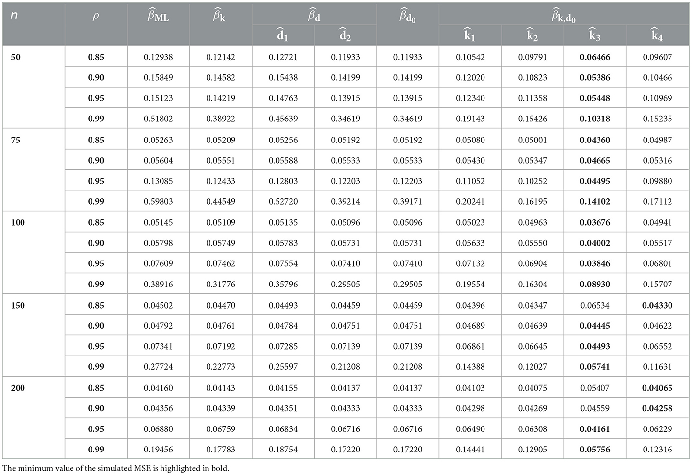
Table 1. MSE values in case of p = 3 and γ = 0.85.

TABLE 2

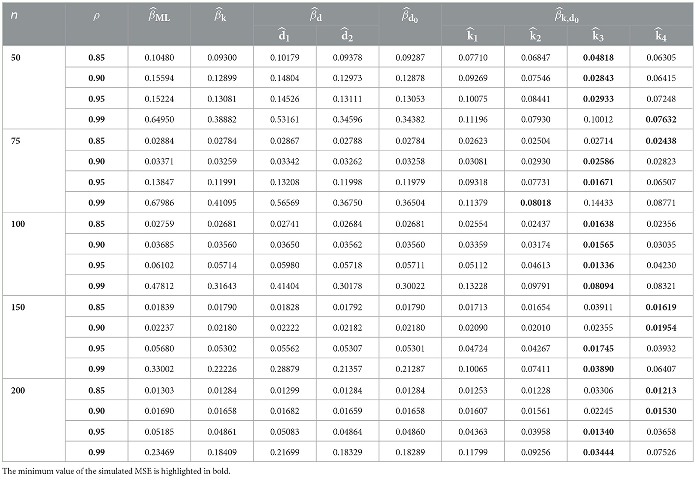
Table 2. MSE values in case of p = 3 and γ = 1.

TABLE 3

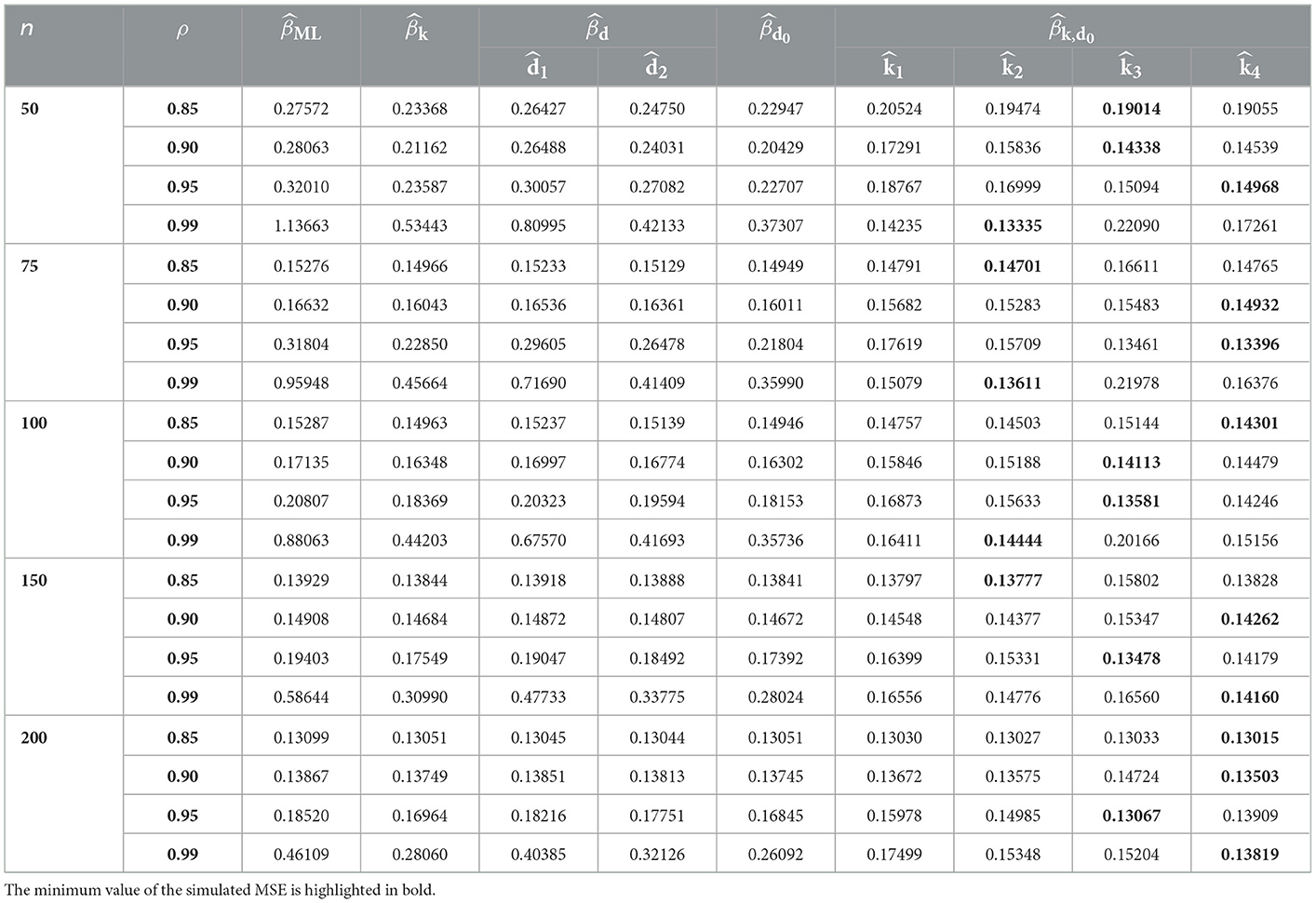
Table 3. MSE values in case of p = 3 and γ = 1.5.

TABLE 4

Table 4. MSE values in case of p = 6 and γ = 0.85.

TABLE 5

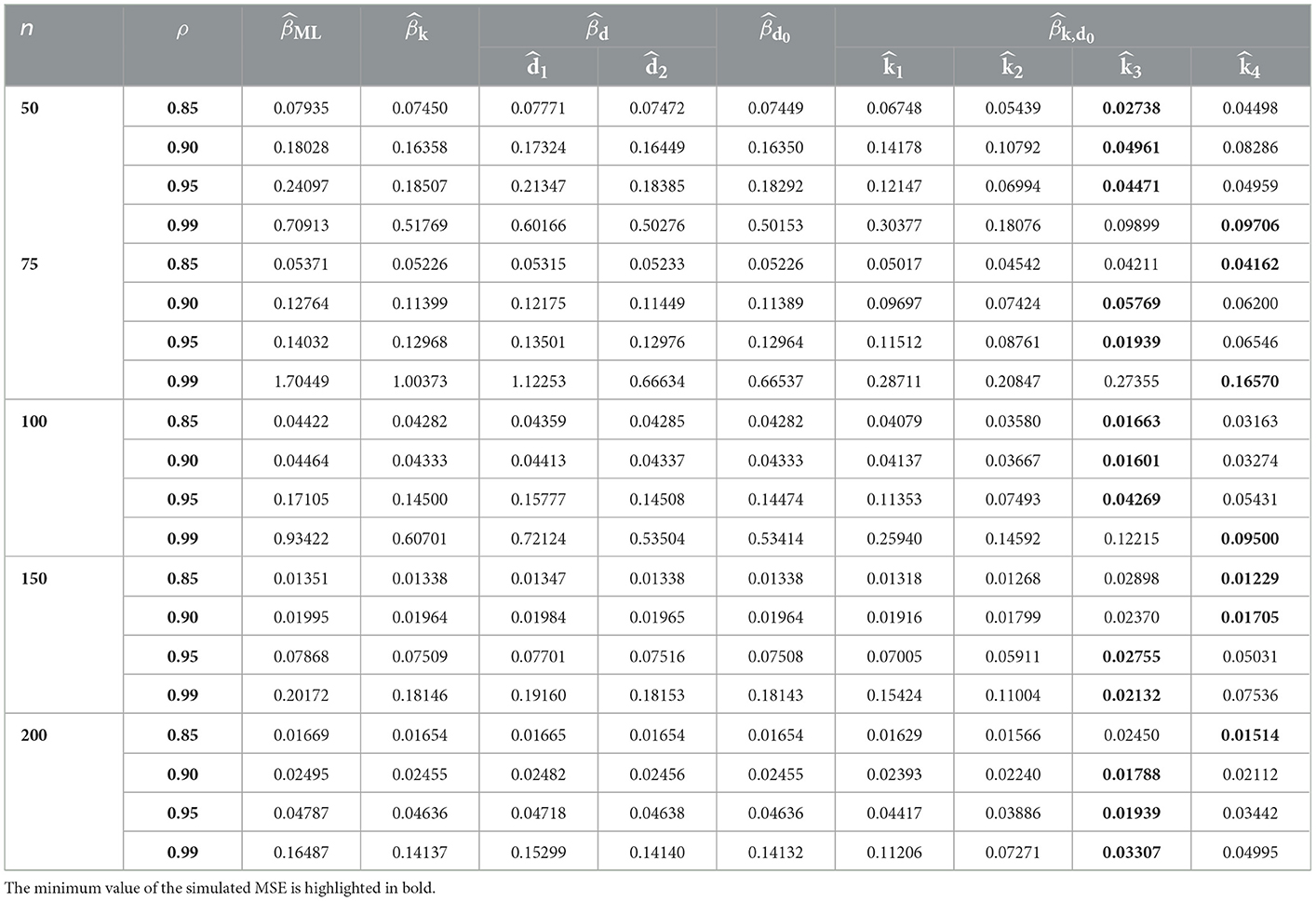
Table 5. MSE values in case of p = 6 and γ = 1.

TABLE 6

Table 6. MSE values in case of p = 6 and γ = 1.5.

TABLE 7

Table 7. MSE values in case of p = 9 and γ = 0.85.

TABLE 8

Table 8. MSE values in case of p = 9 and γ = 1.

TABLE 9

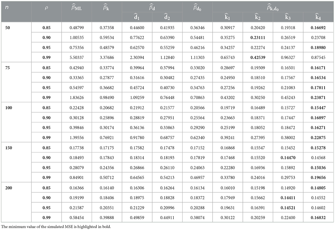
Table 9. MSE values in case of p = 9 and γ = 1.5.

5.3. Relative efficiency

In this sub-section, we use the relative efficiency (RE) measure to study the efficiency of the biased estimators. The RE is derived using the MSE in equation (41) as given by Algamal et al. [35], Farghali et al. [40], and Abonazel and Taha [42] as follows:

$\begin{array}{ll}\text{RE }\left(\hat{\beta }*\right)=\frac{\text{MSE }\left({\hat{\beta }}_{\text{ML}}\right)}{\text{MSE }\left(\hat{\beta }*\right)},& \left(42\right)\end{array}$

where $\widehat{\beta }*$ represents ${\hat{\beta }}_k,{\hat{\beta }}_d,{\hat{\beta }}_{d_0},$ or ${\hat{\beta }}_{{k,d}_0}$. Moreover, the root mean squared error (RMSE) is used as a standard statistical tool for assessing the performance of the estimators. It is calculated using the estimators' MSE as follows:

$\begin{array}{ll}\text{RMSE}=\sqrt{\text{MSE }\left(\hat{\beta }*\right)}& \left(43\right)\end{array}$

Figures 2–5 present RMSE of the CPML, CPR, CPL, CPMOPL, and CPNMTPL estimators and RE of the CPR, CPL, CPMOPL, and CPNMTPL estimators for different levels of the sample sizes (n), correlation degrees between explanatory variables (ρ), the dispersion parameter (γ), and the number of explanatory variables (p), respectively. Figures 2–5 show that the CPML estimator has the largest value, while the proposed estimator CPNMTPL with ${\hat{k}}_2,{\hat{k}}_3,and{\hat{k}}_4$ has the smallest value of RMSE. For relative efficiency, the CPNMTPL estimator with ${\hat{k}}_2,{\hat{k}}_3,and{\hat{k}}_4$ has higher RE values than the other estimators for different levels of n, p, γ, and ρ.

FIGURE 2

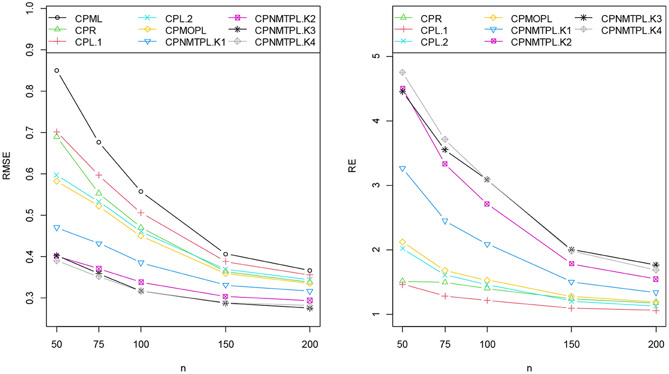
Figure 2. RMSE and RE categorized by levels of sample size.

FIGURE 3

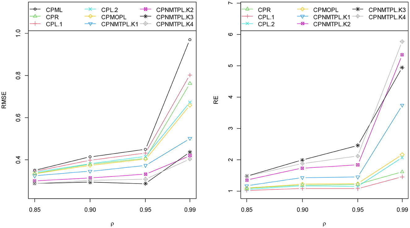
Figure 3. RMSE and RE categorized by levels of the correlation degree between explanatory variables.

FIGURE 4

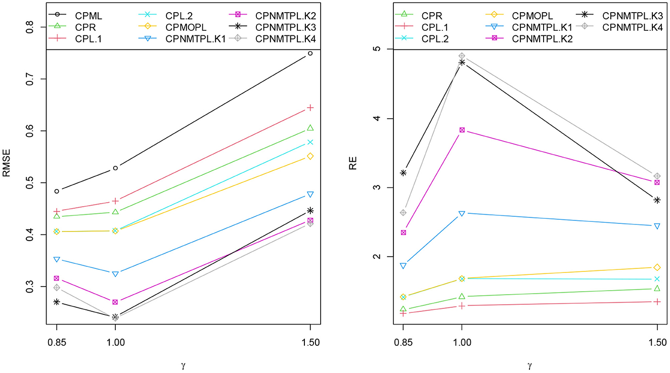
Figure 4. RMSE and RE categorized by dispersion parameter levels.

FIGURE 5

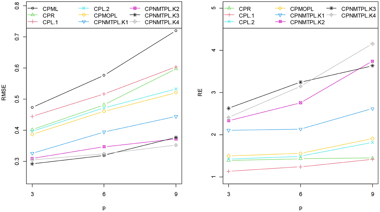
Figure 5. RMSE and RE categorized by the number of explanatory variables.

6. Application

In this section, we use a real dataset from Cameron and Trivedi [43] to estimate a recreation demand function. This dataset was obtained from a survey on the number of recreational boating trips to Somerville Lake, East Texas, in 1980. The response (dependent) variable of this data is the number of recreational boating trips to Somerville Lake in 1980. While there are three explanatory variables as follows: X1: Lake Conroe visit fee, X2: Somerville Lake visit fee, and X3: Houston Lake visit fee. These data are also used by Abonazel and Dawoud [44], the sample size is 179 observations (after removing the outlier values). To check the existence of the multicollinearity problem, correlation coefficients between explanatory variables, variance inflation factor (VIF), and condition number (CN) can be used. All correlation coefficients are greater than 0.90: ρ_{X1, X2} = 0.97, ρ_{X1, X3} = 0.98, ρ_{X2, X3} = 0.94. While the values of the VIF are 157.75, 52.34, and 90.10, and the value of the CN is 29.10. The correlation coefficients, VIF, and CN values confirm the presence of multicollinearity. The VIF values are calculated based on the generalized VIF (GVIF) provided by Fox and Monette [45], as follows:

$\begin{array}{ll}GVIF=\frac{\left|R_1\right|\left|R_2\right|}{\left|R_X\right|},& \left(44\right)\end{array}$

where |·| is the matrix determinant, R₁ is the correlation matrix of a specific set of explanatory variables, R₂ is the correlation matrix of a particular set of explanatory variables, and R_X is the correlation matrix of all the explanatory variables in the model [46]: $R_X={\left(diag\left(V\right)\right)}^{-\frac{1}{2}}V{\left(diag\left(V\right)\right)}^{-\frac{1}{2}}$, where $V=\hat{\gamma }{\left(X^{\prime }\hat{W}X\right)}^{-1}$ is the estimated variance–covariance matrix of ${\hat{\beta }}_{ML}$ and diag(V) is the matrix of the diagonal elements of V. While the CN value is calculated based on the following formula [47]:

$\begin{array}{ll}CN=\sqrt{\frac{{\lambda }_{max}}{{\lambda }_{min}}},& \left(45\right)\end{array}$

where λ_max and λ_min are the largest and smallest eigenvalues of the $X^{\prime }\hat{W}X$ matrix.

First, we have fitted various count data models that are the Poisson, the negative binomial, and the COMP distributions. The Akaike information criterion (AIC) is used to select the best model. AIC values of these models are found to be the Poisson (60.50), the negative binomial (50.61), and the COMP (45.09). We observed that the COMP has a minimum AIC value. This shows that the COMP model is well fitted to this data.

Table 10 presents the estimates of regression coefficients, estimated MSE, and R-squared (R²) for the different estimators. The estimated MSE of the CPML, CPR, CPL, CPMOPL, and CPNMTPL estimators was obtained by equations (8), (13), (18), (23), and (28), respectively, based on the $\hat{\alpha }={\psi }^{\prime }{\hat{\beta }}_{ML}$ and the estimated values of the biasing parameters ($\hat{k},{\hat{d}}_1,{\hat{d}}_2,{\hat{d}}_0,{\hat{k}}_1,{\hat{k}}_2,{\hat{k}}_3,and{\hat{k}}_4$). The R-squared (R²) is calculated based on the following formula [48]:

$\begin{array}{ll}{R}^2=1-\frac{{{\displaystyle \sum }}_{i=1}^n\frac{{(y_i-{\hat{\mu }}_i)}^2}{{\hat{\mu }}_i}}{{{\displaystyle \sum }}_{i=1}^n\frac{{(y_i-\overline{y})}^2}{\overline{y}}},& \left(46\right)\end{array}$

where $\overline{y}=n^{-1}{\sum }_{i=1}^n{y}_i$, ${\hat{\mu }}_i=exp\left(x_i^{\prime }\hat{\beta }\right)$; $\hat{\beta }$ represents ${\hat{\beta }}_{ML},{\hat{\beta }}_k,{\hat{\beta }}_d,{\hat{\beta }}_{d_0},$ and ${\hat{\beta }}_{{k,d}_0}$ to obtain R² for the CPML, CPR, CPL, CPMOPL, and CPNMTPL estimators, respectively.

TABLE 10

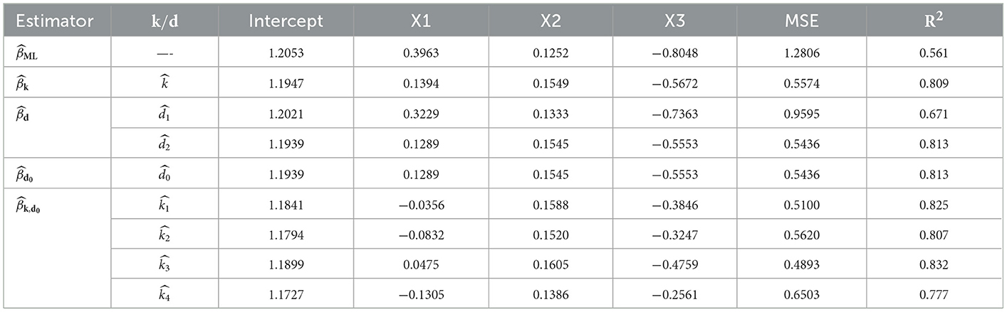
Table 10. Estimated coefficients, MSE, and R².

From Table 10, we note the following:

1. It is noted that the estimated coefficients for the biased estimators [CPR, CPL, CPMOPL, and CPNMTPL(${\hat{k}}_3$)] have the same sign; this suggests that the correlation between each explanatory variable and the response variable remains unchanged from the CPML estimator.

2. The MSE values of the CPR, CPL, CPMOPL, and CPNMTPL estimators are lower than the CPML. However, the CPNMTPL estimator based on the ${\hat{k}}_3$ has the lowest value of MSE.

3. Furthermore, in terms of prediction, the R² value of the proposed CPNMTPL estimator is the greatest among all the used estimators.

Through this dataset, we confirm the theoretical results as follows:

• The required condition of theorem 1 is satisfied for j = 1, 2, 3, 4, $\hat{\gamma }{\sum }_{j=1}^4\left(a_j^2{c}_j^2-{\lambda }_j^2{b}_j^2\right)=4.12e+09>{\sum }_{j=1}^4{\lambda }_j{{\alpha }_j^2\left(k\left(2{\lambda }_j+1\right)+{\lambda }_j\left(1+d_0\right)\right)}^2=1.08e+09$, so the performance of the CPNMTPL estimator is better than the CPML estimator.

• The required condition of theorem 2 is satisfied for j = 1, 2, 3, 4, $\hat{\gamma }{\sum }_{j=1}^4{\lambda }_j\left(a_j^2-b_j^2\right)=3.13e+06>{\sum }_{j=1}^4{\alpha }_j^2\left({\left(k\left(2{\lambda }_j+1\right)+{\lambda }_j\left(1+d_0\right)\right)}^2-k^2{a}_j^2\right)=9.42e+05$, so the performance of the CPNMTPL estimator is better than the CPR estimator.

• The required condition of theorem 3 is satisfied for j = 1, 2, 3, 4, $\hat{\gamma }{\sum }_{j=1}^4\left(e_j^2{c}_j^2-{\lambda }_j^2{b}_j^2\right)=3.29e+09>{\sum }_{j=1}^4{\alpha }_j^2{\lambda }_j\left[{\left(k\left(2{\lambda }_j+1\right)+{\lambda }_j\left(1+d_0\right)\right)}^2-c_j^2{\left(d-1\right)}^2\right]=1.04e+09$, so the performance of the CPNMTPL estimator is better than the CPL estimator.

• The required condition of theorem 4 is satisfied for j = 1, 2, 3, 4, $\hat{\gamma }{\sum }_{j=1}^4\left(f_j^2{c}_j^2-{\lambda }_j^2{b}_j^2\right)=1.10e+09>{\sum }_{j=1}^4{\lambda }_j{\alpha }_j^2\left[{\left(k\left(2{\lambda }_j+1\right)+{\lambda }_j\left(1+d_0\right)\right)}^2-c_j^2{\left(d_0+1\right)}^2\right]=5.00e+08$, so the performance of the CPNMTPL estimator is better than the CPMOPL estimator.

7. Conclusion

In this article, we proposed a new modified two-parameter Liu estimator (CPNMTPL estimator) for the COMP model to deal with the multicollinearity issue. We proved that the proposed CPNMTPL estimator is more efficient than the previously biased estimators (CPR, CPL, and CPMOPL estimators) proposed in the literature. The simulation study and the real data application were conducted to examine the performance of the CPNMTPL estimator and compared it with the CPR, CPL, and CPMOPL estimators. The results of the simulation study and empirical application indicated that the CPNMTPL estimator outperforms these estimators, in terms of the mean squared error (MSE) reduction. Under three values of dispersion, the CPNMTPL estimator, with all biasing parameters, performs better than the CPR, CPL, and CPMOPL estimators when the COMP model contains the multicollinearity issue. In the future study, we will use the generalized cross-validation (GCV) criterion to select the biasing parameters of the proposed estimator, as an extension of Roozbeh [49], to achieve more efficiency.

Data availability statement

The original contributions presented in the study are included in the article/supplementary material, further inquiries can be directed to the corresponding author.

Author contributions

Conceptualization, software, formal analysis, and writing—original draft preparation: ETE, FAA, and MRA. Methodology: ETE, MRA, and IGK. Validation, investigation, and writing—review and editing: FAA, MRA, IGK, and BMGK. Resources: FAA, MRA, and IGK. Visualization: ETE and MRA. Supervision: IGK and BMGK. Project administration: ETE, FAA, MRA, IGK, and BMGK. Funding acquisition: FAA, MRA, and IGK. All authors have read and agreed to the published version of the manuscript.

Acknowledgments

Researchers Supporting Project number (RSPD2023R576), King Saud University, Riyadh, Saudi Arabia.

Conflict of interest

The authors declare that the research was conducted in the absence of any commercial or financial relationships that could be construed as a potential conflict of interest.

Publisher's note

All claims expressed in this article are solely those of the authors and do not necessarily represent those of their affiliated organizations, or those of the publisher, the editors and the reviewers. Any product that may be evaluated in this article, or claim that may be made by its manufacturer, is not guaranteed or endorsed by the publisher.

References

1. Cancho VG, Ortega EM, Barriga GD, Hashimoto EM. The Conway–Maxwell–Poisson-generalized gamma regression model with long-term survivors. J Stat Comput Simul. (2011) 81:1461–81. doi: 10.1080/00949655.2010.491827

CrossRef Full Text | Google Scholar

2. Anan O, Böhning D, Maruotti A. Population size estimation and heterogeneity in capture–recapture data: a linear regression estimator based on the Conway–Maxwell–Poisson distribution. Stat Methods Applic. (2017) 26:49–79. doi: 10.1007/s10260-016-0358-7

CrossRef Full Text | Google Scholar

3. Conway RW, Maxwell WL. A queuing model with state dependent service rates. J Ind Eng Int. (1962) 12:132–6.

PubMed Abstract

4. Shmueli G, Minka TP, Kadane JB, Borle S, Boatwright P. A useful distribution for fitting discrete data: revival of the Conway–Maxwell–Poisson distribution. J R Stat Soc. (2005) 54:127–42. doi: 10.1111/j.1467-9876.2005.00474.x

CrossRef Full Text | Google Scholar

5. Nadarajah S. Useful moment and CDF formulations for the COM–Poisson distribution. Stat Papers. (2009) 50:617–22. doi: 10.1007/s00362-007-0089-9

CrossRef Full Text | Google Scholar

6. Borges P, Rodrigues J, Balakrishnan N, Bazán J. A COM–Poisson type generalization of the binomial distribution and its properties and applications. Stat Prob Lett. (2014) 87:158–66. doi: 10.1016/j.spl.2014.01.019

CrossRef Full Text | Google Scholar

7. Gillispie SB, Green CG. Approximating the Conway–Maxwell–Poisson distribution normalization constant. Statistics. (2015) 49:1062–73. doi: 10.1080/02331888.2014.896919

PubMed Abstract | CrossRef Full Text | Google Scholar

8. Hoerl AE, Kennard RW. Ridge regression: biased estimation for non–orthogonal problems. J Dental Technol. (1970) 12:55–67. doi: 10.1080/00401706.1970.10488634

CrossRef Full Text | Google Scholar

9. Månsson K, Shukur G. A Poisson ridge regression estimator. J Econ Model. (2011) 28:1475–81. doi: 10.1016/j.econmod.2011.02.030

CrossRef Full Text | Google Scholar

10. Månsson K. On ridge estimators for the negative binomial regression model. J Econ Model. (2012) 29:178–84. doi: 10.1016/j.econmod.2011.09.009

PubMed Abstract | CrossRef Full Text | Google Scholar

11. Türkan S, Özel G. A new modified Jackknifed estimator for the Poisson regression model. J Appl Stat. (2016) 43:1892–905. doi: 10.1080/02664763.2015.1125861

CrossRef Full Text | Google Scholar

12. Kaçiranlar S, Dawoud I. On the performance of the Poisson and the negative binomial ridge predictors. J Commun Stat Simul Comput. (2018) 47:1751–70. doi: 10.1080/03610918.2017.1324978

CrossRef Full Text | Google Scholar

13. Zaldivar C. On the performance of some Poisson Ridge Regression estimator FIU Electronic. Theses and Dissertations. (2018). p. 3669.

Google Scholar

14. Rashad NK, Algamal ZY. A new ridge estimator for the Poisson regression model. Iran J Sci Technol Trans Sci. (2019) 45:2921–8. doi: 10.1007/s40995-019-00769-3

CrossRef Full Text | Google Scholar

15. Yehia EG. On the restricted poisson ridge regression estimator. Sci J Appl Mathem Stat. (2021) 9:106–12. doi: 10.11648/j.sjams.20210904.12

CrossRef Full Text | Google Scholar

16. Algamal ZY, Lukman AF, Abonazel MR, Awwad FA. Performance of the Ridge and Liu Estimators in the zero-inflated Bell Regression Model. J Mathem. (2022) 2022:9503460. doi: 10.1155/2022/9503460

CrossRef Full Text | Google Scholar

17. Akram MN, Abonazel MR, Amin M, Kibria BG, Afzal N. A new Stein estimator for the zero-inflated negative binomial regression model. Concurr Comput. (2022) 34:e7045. doi: 10.1002/cpe.7045

CrossRef Full Text | Google Scholar

18. Liu K. A new class of biased estimate in linear regression. J Commun Stat Theory Methods. (1993) 22:393–402. doi: 10.1080/03610929308831027

CrossRef Full Text | Google Scholar

19. Månsson K, Kibria BM, Sjölander P, Shukur G. Improved Liu estimators for the Poisson regression model. Int J Stat Prob. (2012) 1:2. doi: 10.5539/ijsp.v1n1p2

CrossRef Full Text | Google Scholar

20. Månsson K. Developing a Liu estimator for the negative binomial regression model: method and application. J Stat Comput Simul. (2013) 83:1773–80. doi: 10.1080/00949655.2012.673127

CrossRef Full Text | Google Scholar

21. Amin M, Akram MN, Kibria BM. A new adjusted Liu estimator for the Poisson regression model. J Concurr Computat Pract Exper. (2021) 33:e6340. doi: 10.1002/cpe.6340

CrossRef Full Text | Google Scholar

22. Akram MN, Amin M, Sami F, Mastor AB, Egeh OM, Muse AH. A new Conway Maxwell–Poisson Liu regression estimator—method and application. J Mathem. (2022) 2022:3323955. doi: 10.1155/2022/3323955

PubMed Abstract | CrossRef Full Text | Google Scholar

23. Sami F, Amin M, Akram MN, Butt MM, Ashraf B. A modified one parameter Liu estimator for Conway-Maxwell Poisson response model. J Stat Comput Simulat. (2022) 92:2448–66. doi: 10.1080/00949655.2022.2037136

CrossRef Full Text | Google Scholar

24. Yang H, Chang X. A new two-parameter estimator in linear regression. Communic Stat Theory Methods. (2010) 39:923–34. doi: 10.1080/03610920902807911

CrossRef Full Text | Google Scholar

25. Wu J. An unbiased two-parameter estimation with prior information in linear regression model. Sci World J. (2014) 2014:679835. doi: 10.1155/2014/206943

PubMed Abstract | CrossRef Full Text | Google Scholar

26. Omara TM. Modifying two-parameter ridge liu estimator based on ridge estimation. Pakistan J Stat Oper Res. (2019) 15:881–890. doi: 10.18187/pjsor.v15i4.2575

CrossRef Full Text | Google Scholar

27. Dawoud I, Abonazel MR, Awwad FA. Modified Liu estimator to address the multicollinearity problem in regression models: a new biased estimation class. Sci African. (2022) 17:e01372. doi: 10.1016/j.sciaf.2022.e01372

CrossRef Full Text | Google Scholar

28. Awwad FA, Odeniyi KA, Dawoud I, Algamal ZY, Abonazel MR, Kibria BG, et al. New Two-Parameter Estimators for the Logistic Regression Model with Multicollinearity. WSEAS Trans Mathem. (2022) 21:403–14. doi: 10.37394/23206.2022.21.48

CrossRef Full Text | Google Scholar

29. Algamal ZY, Abonazel MR. Developing a Liu-type estimator in beta regression model. Concurr Comput. (2022) 34:e6685. doi: 10.1002/cpe.6685

CrossRef Full Text | Google Scholar

30. Guikema SD, Goffelt JP. A flexible count data regression model for risk analysis. J Risk Anal. (2008) 28:213–23. doi: 10.1111/j.1539-6924.2008.01014.x

PubMed Abstract | CrossRef Full Text | Google Scholar

31. Sami F, Amin M, Butt BM. On the ridge estimation of the Conway–Maxwell Poisson regression model with multicollinearity: Methods and applications. J Concurr Computat Pract Exper. (2021) 34:1–16. doi: 10.1002/cpe.6477

CrossRef Full Text | Google Scholar

32. Segerstedt B. On ordinary ridge regression in generalized linear models. J Commun Stat Theory Methods. (1992) 21:2227–46. doi: 10.1080/03610929208830909

CrossRef Full Text | Google Scholar

33. Rasheed HA, Sadik NJ, Algamal ZY. Jackknifed Liu–type estimator in the Conway–Maxwell Poisson regression model. Int J Nonlinear Anal Appl. (2022) 13:3153–3168. doi: 10.22075/IJNAA.2022.6064

CrossRef Full Text | Google Scholar

34. Abonazel MR. New Modified Two–Parameter Liu Estimator for the Conway–Maxwell Poisson Regression Model. J Stat Comput Simul. (2023) 1–30. doi: 10.1080/00949655.2023.2166046

CrossRef Full Text | Google Scholar

35. Algamal ZY, Abonazel MR, Awwad FA, Tag Eldin E. Modified jackknife ridge estimator for the conway-maxwell-poisson model. Sci African. (2023) 19:e01543. doi: 10.1016/j.sciaf.2023.e01543

CrossRef Full Text | Google Scholar

36. Kibria BM, Lukman AF. A new ridge–type estimator for the linear regression model: simulations and applications. J Scientifica. (2020) 2020:1–16. doi: 10.1155/2020/9758378

PubMed Abstract | CrossRef Full Text | Google Scholar

37. Lukman AF, Algamal ZY, Kibria BG, Ayinde K. The KL estimator for the inverse Gaussian regression model. J Concur Computat Pract Exper. (2021) 33:e6222. doi: 10.1002/cpe.6222

CrossRef Full Text | Google Scholar

38. Kibria BM. Performance of some new ridge regression estimators. J Commun Stat Simul Comput. (2003) 32:419–35. doi: 10.1081/SAC-120017499

CrossRef Full Text | Google Scholar

39. Abonazel MR, Algamal ZY, Awwad FA, Taha IM. A new two-parameter estimator for beta regression model: method, simulation, and application. Front Appl Mathem Stat. (2022) 7:780322. doi: 10.3389/fams.2021.780322

CrossRef Full Text | Google Scholar

40. Farghali RA, Qasim M, Kibria BG, Abonazel MR. Generalized two-parameter estimators in the multinomial logit regression model: methods, simulation and application. Communic Stat Simul Comput. (2021) 1–16. doi: 10.1080/03610918.2021.1934023

CrossRef Full Text | Google Scholar

41. Abonazel MR, Dawoud I, Awwad FA, Lukman AF. Dawoud–Kibria estimator for beta regression model: simulation and application. Front Appl Mathem Stat. (2022) 8:775068. doi: 10.3389/fams.2022.775068

CrossRef Full Text | Google Scholar

42. Abonazel MR, Taha IM. Beta ridge regression estimators: simulation and application. Commun Stat Simul Comput. (2021) 1–13. doi: 10.1080/03610918.2021.1960373

CrossRef Full Text | Google Scholar

43. Cameron AC, Trivedi PK. Regression Analysis of Count Data, 2^nd Edition, Econometric Society Monograph No. 53. Cambridge University Press. (2013) p. 1998. doi: 10.1017/CBO9780511814365

CrossRef Full Text | Google Scholar

44. Abonazel MR, Dawoud I. Developing robust ridge estimators for Poisson regression model. J Concurr Computat Pract Exper. (2022) 34:e6979. doi: 10.1002/cpe.6979

CrossRef Full Text | Google Scholar

45. Fox J, Monette G. Generalized collinearity diagnostics. J Am Stat Assoc. (1992) 87:178–83. doi: 10.1080/01621459.1992.10475190

CrossRef Full Text | Google Scholar

46. Özkale MR. The red indicator and corrected VIFs in generalized linear models. Commun Stat Simul Comput. (2021) 50:4144–70. doi: 10.1080/03610918.2019.1639740

CrossRef Full Text | Google Scholar

47. Riley JD. Solving systems of linear equations with a positive definite, symmetric, but possibly ill-conditioned matrix. Mathem Tables Other Aids Comput. (1955) 9:96–101. doi: 10.1090/S0025-5718-1955-0074915-1

CrossRef Full Text | Google Scholar

48. Cameron AC, Windmeijer FA. R-squared measures for count data regression models with applications to health-care utilization. J Busin Econ Stat. (1996) 14:209–20. doi: 10.1080/07350015.1996.10524648

CrossRef Full Text | Google Scholar

49. Roozbeh M. Optimal QR-based estimation in partially linear regression models with correlated errors using GCV criterion. Comput Stat Data Anal. (2018) 117:45–61. doi: 10.1016/j.csda.2017.08.002

CrossRef Full Text | Google Scholar