Least square-support vector machine based brain tumor classification system with multi model texture features

Radiologists confront formidable challenges when confronted with the intricate task of classifying brain tumors through the analysis of MRI images. Our forthcoming manuscript introduces an innovative and highly effective methodology that capitalizes on the capabilities of Least Squares Support Vector Machines (LS-SVM) in tandem with the rich insights drawn from Multi-Scale Morphological Texture Features (MMTF) extracted from T1-weighted MR images. Our methodology underwent meticulous evaluation on a substantial dataset encompassing 139 cases, consisting of 119 cases of aberrant tumors and 20 cases of normal brain images. The outcomes we achieved are nothing short of extraordinary. Our LS-SVM-based approach vastly outperforms competing classifiers, demonstrating its dominance with an exceptional accuracy rate of 98.97%. This represents a substantial 3.97% improvement over alternative methods, accompanied by a notable 2.48% enhancement in Sensitivity and a substantial 10% increase in Specificity. These results conclusively surpass the performance of traditional classifiers such as Support Vector Machines (SVM), Radial Basis Function (RBF), and Artificial Neural Networks (ANN) in terms of classification accuracy. The outstanding performance of our model in the realm of brain tumor diagnosis signifies a substantial leap forward in the field, holding the promise of delivering more precise and dependable tools for radiologists and healthcare professionals in their pivotal role of identifying and classifying brain tumors using MRI imaging techniques.

1 Introduction

Pathological anomalies that originate in the brain encompass a spectrum of conditions, with brain tumors standing as a significant category [1]. These tumors exhibit varying degrees of aggressiveness, leading to their classification as either benign (non-cancerous) or malignant (cancerous). To systematically differentiate these tumors based on their malignancy, the World Health Organization (WHO) has devised a comprehensive grading system, spanning from grade 1 to grade 4 [2]. Meningiomas and pituitary tumors categorized as non-cancerous often manifest with lower grades, displaying limited tendencies to infiltrate the surrounding healthy brain cells [3]. This characteristic sets them apart from their malignant counterparts, which showcase heightened aggressiveness and a propensity to infiltrate adjacent brain tissues. At the pinnacle of malignant brain tumors stands glioblastoma (GBM), a particularly prevalent and perilous manifestation. This formidable tumor typically receives a grade 4 designation within the WHO grading system, indicating its highly malignant nature and notoriously bleak prognosis [4, 5].

Brain tumor emerges from a disruption in the intricate balance of cell growth within the brain, resulting in uncontrolled proliferation [6]. Unfortunately, the toll of brain tumors in terms of lives claimed has reached unprecedented heights. Most benign tumors manifest as cysts and are entirely treatable without the risk of recurrence post-treatment due to the absence of cancerous cells. These tumors exhibit a more subdued aggressiveness and refrain from infiltrating neighboring tissues. In contrast, malignant tumors shelter cancerous cells and exhibit an elevated level of aggression, showcasing rapid growth rates that exert significant pressure on the brain, thus carrying far graver implications. Malignant tumors not only infect the surrounding brain tissue, but they also possess the ominous potential to metastasize to distant regions of the body, including the spinal cord [7, 8].

The identification of brain tumors presents a formidable challenge, demanding the expertise of extensively trained medical professionals. However, the present techniques employed for detecting brain tumors suffer from several drawbacks—consuming considerable time, incurring high costs, and occasionally yielding inaccuracies in specific scenarios [9]. Magnetic Resonance Imaging (MRI), Magnetic Resonance Spectroscopy (MRS), and Computed Tomography (CT) are among the various medical imaging techniques that are routinely being employed to pinpoint and characterize brain tumors. A multitude of factors, including the presumed tumor type and its specific location, demand meticulous deliberation when choosing the suitable imaging modality. These decisions pivot on the patient's medical background and the accessibility to imaging equipment. In certain instances, a combination of imaging methodologies might be deployed to achieve a precise diagnosis. This underscores the pressing need for a more streamlined and precise approach to brain tumor detection.

Given the dynamic nature of brain lesions, characterized by a spectrum of attributes encompassing differing sizes, intricate structures, varied locations, temporal evolution, and distinctive imaging characteristics, the endeavor to employ computer-based methods for the detection and segmentation of these lesions remains an enduring challenge [10]. Nonetheless, with growing advancements in medical imaging technology, the diagnosis of conditions such as Brain tumors, Alzheimer's disease, multiple sclerosis, schizophrenia, and various white matter lesions has been substantially facilitated through the application of brain magnetic resonance imaging (MRI) [11].

Presently, clinical and radiological data play an integral role in the diagnosis and treatment of brain tumors and magnetic resonance imaging (MRI) stays at the heart of evaluating patients with brain tumors [11]. Nevertheless, conventional imaging techniques exhibit notable limitations in consistently delineating tumor extent, accurately predicting tumor grade, and effectively assessing treatment efficacy [12, 13]. Ongoing enhancements in imaging methodologies are strategically aimed at refining the detection, assessment, and therapeutic strategies for brain tumors [12, 13]. The wealth of information furnished by radiographic images has concurrently paved the path for the emergence of novel avenues in the realm of image analysis [14].

In image analysis, categorizing and segmenting brain tumors is crucial. Manual and computer-assisted methods exist, but manual classification is laborious and prone to errors. Advanced medical image processing [15] leverages modalities like PET, CT [16], ultrasound, MRI, and X-ray for noninvasive solutions. In the realm of medical applications, a pivotal role of digital image processing lies in enhancing source images. Images from diverse medical technologies, such as X-ray, MRI, and X-ray-based CT, may exhibit regions of blurriness or noise. To rectify this, low-level image processing techniques like denoising, sharpening, and edge detection are employed. These algorithms are finely tuned with specific parameter values tailored to the specific context, thereby augmenting the informative content accessible to interpreting medical practitioners [17].

Artificial intelligence (AI) has rapidly emerged as a transformative force across various domains, including education [18, 19], finance [20], agriculture [21–26], healthcare [27, 28], and beyond [29, 30]. Healthcare benefits from AI-driven diagnostics, predictive analytics, and telemedicine, offering improved patient care and resource allocation. The proliferation of AI has reshaped these sectors, promising efficiency gains, cost savings, and enhanced decision support, ultimately improving the quality of services and the overall human experience. As AI continues to advance, its potential applications and impact on diverse industries are bound to expand further [31–33].

Deep neural networks (DNNs) are transformative in diverse domains like healthcare [34, 35]. In brain tumor detection, DNNs automatically extract meaningful insights from vast medical imaging data. This subset of machine learning imitates human brain structure, learning progressively intricate features through interconnected layers [36]. DNNs analyze and pinpoint brain tumor patterns, including size, shape, and location, learning from extensive datasets [18, 36–38]. Notably, they adapt to varied imaging conditions and can fuse multiple modalities, enhancing accuracy in diagnosis. Convolutional neural networks (CNNs) specifically process brain imaging data, learning tumor indicators through convolutional layers [39, 40]. CNNs master patterns through weighted adjustment, reliably identifying brain tumors.

Researchers have made numerous attempts to enhance brain tumor identification accuracy recently. Prior studies evaluating the clinical significance of each MR sequence in prediction and detection prove invaluable [41, 42]. Utilizing MRI and CT, researchers distinguished tumors from other anomalies. MR spectroscopy extensively characterized brain tumors across diverse studies. Saeedi et al. [43] proposed 2D CNN and auto-encoder network for classifying glioma, meningioma, pituitary tumors, and healthy brains using 3,264 MRI images. Their average recall was 95% and 94%, with ROC AUC of 0.99 or 1. Comparing machine learning methods, K-Nearest Neighbors (KNN) achieved 86% accuracy, while Multilayer Perceptron (MLP) had the lowest (28%). The 2D CNN demonstrated optimal tumor classification accuracy and practicality for clinical use. Sharma et al. [44] introduced a brain tumor detection method using CNN's pretrained data sets with ResNet50 feature extraction and augmentation. In their study, Qin et al. [45] employed the SVM classifier for brain tumor detection. Initially, they extracted MR image features through the HOG algorithm, comparing them with features obtained using wavelet transform. Additionally, they utilized SVM with the a-norm loss function for classification, which improved the detection significantly at a faster rate due to its sparse nature. Mathew and Anto [46] aimed to develop an efficient tumor detection and classification system using MRI preprocessing, discrete wavelet transform-based feature extraction, and Support Vector Machine (SVM) for segmentation and classification.

A transfer learning-based fine-tuning approach was employed by Zulfiqar et al. [47] for classification of tumors and the pre-trained EfficientNet demonstrated remarkable results with EfficientNetB2 as a backbone. It achieved an overall test accuracy of 98.86%, precision of 98.65%, recall/sensitivity of 98.77%, and F1-score of 98.71%. The fine-tuned EfficientNetB2 proved to be lightweight, computationally efficient, and exhibited good generalization capabilities. Mehnatkesh et al. [48] introduced an optimization-based deep Convolutional ResNet model, enhanced by an innovative evolutionary algorithm, for automatic architecture and hyperparameter optimization without human intervention. The approach achieved an impressive average accuracy of 0.98694, showcasing the effectiveness of IACO-ResNet for automatic brain tumor classification. A fusion of Naïve Bayes, Support Vector Machine, and K-Nearest Neighbor algorithms was employed by Ghafourian et al. [49] to classify extracted features for brain tumor detection. Individual algorithm outputs were integrated for the final model. Results indicated 98.61% average accuracy, 95.79% sensitivity, and 99.71% specificity on the BRATS 2014 dataset. Similarly, on the BTD20 database, the method achieved 99.13% accuracy, 99% sensitivity, and 99.26% specificity.

A deep learning-based model (DLBTDC-MRI) was proposed by Mohan et al. [50] for automated brain tumor detection and classification using MRI data. The method involved preprocessing, segmentation using “chicken swarm optimization” (CSO), and Residual Network (ResNet)-based feature extraction. DLBTDC-MRI showed superior performance on the BRATS 2015 dataset, outperforming other methods in various aspects. Vankdothu and Hameed [51] focused on CT-based brain tumor segmentation using preprocessing and classification techniques. The researchers used ANFIS and SVM classifiers for classification and claim that FCM clustering with hybrid optimization (SSO-GA) achieved a high accuracy of 99.24% in tumor segmentation. The study by Qader et al. [52] presented an enhanced Deep Convolutional Neural Network (DCNN) named G-HHO, utilizing improved Harris Hawks Optimization (HHO) and Gray Wolf Optimization (GWO). Employing Otsu thresholding for tumor segmentation, it achieves 97% accuracy on 2,073 augmented MRI images, surpassing existing methods in terms of accuracy, execution time, and memory usage.

The existing literature on brain tumor classification predominantly focuses on various machine learning and deep learning techniques. However, there is a gap in research concerning the utilization of Least Squares-Support Vector Machine (LS-SVM) in combination with multi-model texture features for brain tumor classification. This proposed approach offers a unique perspective by combining an efficient classification algorithm with advanced texture analysis, potentially leading to improved accuracy and diagnostic capabilities.

This study introduces an innovative methodology for classifying brain tumors in MRI images, utilizing Least Squares Support Vector Machines (LS-SVM) in conjunction with Multi-Scale Morphological Texture Features (MMTF) extracted from T1-weighted MR images. The methodology is rigorously evaluated on a dataset of 139 cases, comprising 119 aberrant tumor cases and 20 normal brain images. The results demonstrate exceptional performance, with the LS-SVM-based approach outperforming alternative classifiers, achieving an accuracy rate of 98.97%, a 3.97% improvement over other methods. The study emphasizes LS-SVM's dominance, precision with zero False Positives, and heightened sensitivity with only one False Negative. The findings suggest a significant advancement in brain tumor diagnosis, holding promise for more accurate tools in medical imaging. The commitment to open access for the code on GitHub enhances the study's transparency and reproducibility for the research community. The contributions of this study are as follows:

• Innovative Methodology: Introduces a novel methodology that leverages the capabilities of Least Squares Support Vector Machines (LS-SVM) along with Multi-Scale Morphological Texture Features (MMTF) for the classification of brain tumors in MRI images, offering a fresh approach to a challenging problem.

• Exceptional Classification Accuracy: Achieves an outstanding accuracy rate of 98.97%, showcasing the superior performance of the LS-SVM-based approach compared to alternative classifiers. This high accuracy is crucial for enhancing the reliability of brain tumor diagnosis in medical imaging.

• LS-SVM Dominance: Establishes the clear dominance of LS-SVM over other neural network-based classifiers, including Support Vector Machines (SVM), Radial Basis Function (RBF), and Artificial Neural Networks (ANN), across multiple performance metrics, emphasizing its effectiveness in accurately classifying brain regions.

• Precision and Sensitivity: Highlights LS-SVM's precision by achieving zero False Positives, reducing the risk of unnecessary interventions, and its exceptional sensitivity with only one False Negative, demonstrating its capability to detect positive instances crucial in medical applications.

• Promise for Advancing Medical Imaging: Positions the proposed methodology as a substantial leap forward in the field of brain tumor diagnosis, holding the promise of delivering more precise and dependable tools for radiologists and healthcare professionals, ultimately contributing to advancements in medical imaging techniques.

2 Materials and methods

Any computer-aided diagnostic (CAD) or medical decision support system necessitates three core components: segmentation, feature extraction, and classification. In the context of brain tumor identification in medical images, a range of computer-aided techniques (CATs) has been employed, encompassing both automatic and semi-automatic segmentation methods. This paper provides an overview of CAD systems designed for the classification of brain tumors using MRI images, elucidating the theoretical foundations and guiding principles governing feature extraction and classification methodologies. A comprehensive flowchart shown in Figure 1 illustrates the functioning of the proposed CAD system for the detection and classification of brain tumors. The pivotal constituents of this brain tumor classification system encompass pre-processing, segmentation, feature extraction, feature reduction, and classification. Within the pre-processing module, critical operations such as noise elimination, skull stripping, and image enhancement are conducted. To achieve precise tissue segmentation, covering white matter, gray matter, and cerebrospinal fluid (CSF), three distinct algorithms are employed: thresholding, independent component analysis (ICA), and spectral clustering. The feature categorization stage employs a variety of machine learning techniques to discern images as either normal or abnormal.

FIGURE 1

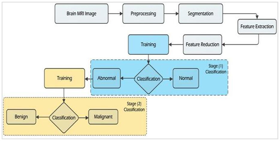
Figure 1. Workflow diagram of the proposed methodology.

Emphasizing the two-stage categorization process, the flowchart visually illustrates the multiple phases within the system. The first stage centers on the detection of brain tumors, while the second stage revolves around distinguishing between benign and malignant tumors. This flowchart comprehensively outlines the system's workflow, with a particular focus on the crucial steps essential for the timely detection and classification of brain tumors.

2.1 Preprocessing

In the realm of image processing, preprocessing plays a pivotal role in approximating the original clean image by effectively mitigating noise from a noisy image. The primary objective of any denoising algorithm is to diminish noise while preserving essential texture and edge characteristics. Denoising techniques predominantly belong to one of three categories: those operating in the spatial domain, those leveraging transformation techniques, or those rooted in dictionary learning.

Our recommended preprocessing methodology encompasses several crucial stages, encompassing noise removal, image enhancement, and skull stripping. Commencing with the utilization of the Medical Picture Processing and Visualization (MIPAV) program, the initial step involves the extraction of the skull from the MRI image. Subsequently, grayscale MR images undergo a noise reduction and image smoothing process, effectively eliminating unwanted noise and enhancing overall image quality. This preprocessing procedure is indispensable in generating a clear, high-fidelity image that serves as the foundational basis for subsequent analysis and interpretation.

2.1.1 Noise removal

The primary objective of image denoising is the removal of undesirable noise while preserving the inherent structure of the image. This is achieved through a combination of wavelet-based noise thresholding techniques and the bilateral filter. As per Equation (1), the initial step involves subtracting the input image from the output of the Bilateral Filter:

$\begin{array}{ll}\text{BS}=\text{NI}-\text{BF}& (1)\end{array}$

In the context of the provided equation, we designate the image obtained through normalization without any noise control adjustments as “NI.” Conversely, “BF” represents the result of applying bilateral filtering to the image. Through the use of bilateral filtering, it is possible to diminish noise in an image while simultaneously preserving vital attributes such as edges and boundaries. It's worth highlighting that the normalized image (NI) retains both the image's information and an amplified level of noise due to the division process employed.

Considering this newfound understanding, Equation (2) provides an alternative representation for the variable BS. This equation, encompassing the preceding operations, can be expressed as follows:

$\begin{array}{ll}BS=I_D-I_N& (2)\end{array}$

Where ID stands for the image details and IN for the noise in the image.

To better identify and separate the noise component from BS, Equation (3) undergoes a transformation into the wavelet domain. This transformation allows us to express the equation in a different manner, facilitating the detection and isolation of noise.

$\begin{array}{ll}Iwd=w+N\omega & (3)\end{array}$

In this context, we denote the authentic wavelet coefficient as “w,” while the wavelet coefficient affected by noise is labeled as “Iwd.” Additionally, “N” signifies the independent noise component. The process of thresholding Iwd is a crucial step in estimating the true wavelet coefficient, “w,” with the aim of minimizing mean square error (MSE).

Equation (4) gives the threshold calculated by minimizing Bayesian risk.

$\begin{array}{ll}{T}_h=\frac{{\sigma }^2}{{\sigma }_{\omega }^2}& (4)\end{array}$

Where 2, which is described in Equation (5), is the noise variance calculated for the sub-band SS1 by a robust median estimator.

$\begin{array}{ll}\widehat{\sigma }=\frac{Median(\left|I_{wd(i,j)}\right|)}{0.6745},I_{wd(i,j)}\in (S{S}_1)& (5)\end{array}$

and the wavelet coefficient's variance is given in Equation (6).

$\begin{array}{l}\widehat{\sigma }w=max(\widehat{\sigma }{y}^2-{\widehat{\sigma }}^2,0)\\ \widehat{\sigma }{y}^2=\frac{1}{BS}{\displaystyle \sum _{i,j=1}^{B,S}}{I}^{2}wdi,j& (6)\end{array}$

Where the wavelet reconstruction process entails the estimation and representation of image features as “D,” derived from the accurate estimation “w.” This “D” is then combined with the bilaterally filtered image to generate the denoised image.

Figure 2 illustrates image denoising using bilateral filtering. The top row showcases the original MRI FLAIR images, while the bottom row exhibits the images after the denoising process.

FIGURE 2

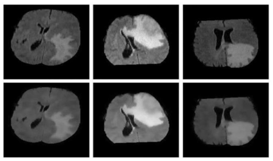
Figure 2. The original and preprocessed images for comparison.

2.1.2 Skull-stripping

Skull stripping is a critical stage in the preprocessing of brain images, involving the removal of the scalp, skull, and Dura mater. To ensure an accurate evaluation of the brain's structure, it is imperative to eliminate non-brain tissues, particularly the Dura mater. Neglecting to exclude non-brain structures could lead to misinterpretations, complicating the process of detection and analysis, thus consuming valuable time. Distinguishing between non-cerebral and intracranial tissues during skull stripping can be challenging, as they often exhibit similar intensity characteristics. Figure 3 offers a visual representation of the skull stripping procedure.

FIGURE 3

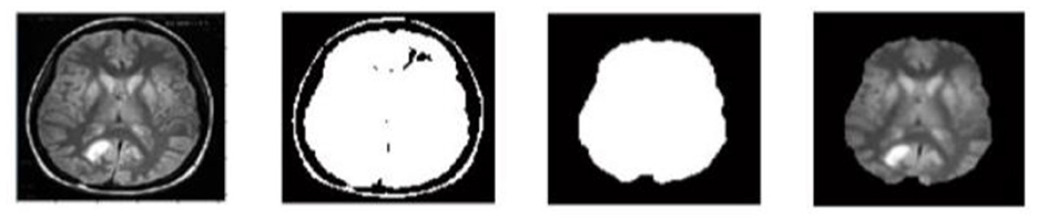
Figure 3. The removal of the skull for an MRI brain imaging.

2.2 Segmentation

In the realm of medical image processing, segmentation emerges as a pivotal yet challenging task. Its primary objective revolves around delineating object boundaries within an image and subsequently extracting these objects. In the proposed system for cancer classification, segmentation relies on the utilization of the thresholding method. Central to this process is the identification of cancerous regions, a task contingent upon preprocessing and segmentation.

In the preprocessing phase, the input image undergoes filtration to attenuate noise and enhance overall image quality. This study employs a Gaussian filter, adept at effectively diminishing visual noise while preserving crucial image elements. Additionally, skull-stripping emerges as a pivotal segmentation step in the domain of medical brain imaging, entailing the separation of the brain from surrounding skull and tissues. Specifically, this procedure targets the scalp, skull, and Dura regions of the brain.

The segmentation procedure encompasses the following steps:

1. Conversion of the MRI image into a binary image through thresholding.

2. Application of morphological techniques to refine the detected region.

3. Identification of the tumor region within the image.

2.2.1 Thresholding through binarization

Image binarization is a technique employed to convert a grayscale image, characterized by a spectrum of gray levels (up to 256), into a binary representation. During this process, the gray-level value of each pixel in the enhanced image is determined. Image binarization is achieved by partitioning the input image based on a predefined threshold value. If a pixel's value surpasses the threshold, it is assigned the value “1;” otherwise, it is assigned the value “0.” Mathematically, this process is depicted by Equation (7), which elucidates the procedure of image binarization.

$\begin{array}{ll}{\text{B}}_{\text{Binary }}(\text{x},\text{y})\text{=}\{\begin{array}{l}\text{0},\text{ if }{\text{B}}_{\text{grey}}(\text{x},\text{y})\text{=}<\text{ Threshold T}\\ \text{1},\text{ Otherwise}\end{array}& (7)\end{array}$

The determination of the threshold value (T) can be achieved through the following steps:

i. Begin by establishing an initial threshold value, denoted as T, derived from the average intensity value of the image.

ii. Utilizing this initial threshold value T, partition the original image into two distinct regions, denoted as R1 and R2.

iii. Calculate the mean values of the two distinct regions, resulting in M1 and M2, respectively.

iv. Update the threshold value T by averaging the means M1 and M2.

v. Iterate through steps ii to iv until successive calculations of the mean values M1 and M2 no longer exhibit any change.

The objective of this iterative process is to identify the optimal threshold value that effectively segregates the image into discrete segments based on their intensity levels. The repetition of these steps ensures the consistency of mean values within the segmented regions, ultimately leading to the attainment of a stable threshold value.

2.2.2 Morphological operation

In image processing, morphological techniques serve as potent tools for accomplishing tasks such as closing gaps and enhancing regions within binarized images [53]. These processes are applied to binarized images using binary morphological operators, primarily aimed at enhancing image quality by eliminating noise and artifacts. The method presented here employs various morphological operators, including closing, opening, erosion, and dilation, with a particular emphasis on the erosion operation.

During the erosion operation on an image G, which is binary with labels of 0 and 1, if the result of convolving X with G, centered at pixel i, falls below a predetermined threshold, the value of pixel i in the image G is changed from 1 to 0. This operation is executed using a structural element X. In our method, this threshold is defined as the proportion of X that corresponds to the number of pixels designated as 1 by the structural element's own labeling element.

Equation (8) underscores the significance of the structuring element, often referred to as the erosion kernel, in determining how erosion influences the boundaries of specific objects within the image.

$\begin{array}{ll}\text{IE}=\text{imerode}(\text{G},\text{X})& (8)\end{array}$

2.2.3 Identification of the tumor region

The region properties function plays a crucial role in pinpointing the primary regions of the tumor. Even after executing the erosion procedure, there may still be undesirable small segments in the image, such as noise and holes. The region props function is employed to ascertain the area of these undesirable segments. If the area of a segment is found to be < 0.8, it is filled with black pixels. These segments are then subjected to further stages, including feature extraction and classification, to determine whether they correspond to tumor or normal regions.

Figure 4 displays the two input images alongside their corresponding pre-processed versions. Subsequently, a skull stripping algorithm is applied to eliminate the skull from the previously processed image. Following this, binarization is employed to create a collection of segments. The image then undergoes an erosion procedure to eliminate noisy regions. The region properties function is utilized to identify and subsequently remove unwanted segments based on their area property. As illustrated in Figure 4, the resulting region is later utilized in subsequent steps to ascertain whether it belongs to a tumor region.

FIGURE 4

Figure 4. The region segmentation procedure in detail.

2.3 Extraction process for multi modal texture features

To ensure the robustness of our system in comparison to using the original pixel data, it becomes imperative to carefully select the most appropriate features for extraction from the analyzed images. This task gains heightened significance, especially considering the intended application. Texture-based feature extraction techniques emerge as highly effective for extracting characteristics from medical images, which often exhibit both repetitive and non-repetitive patterns. These techniques are well-recognized for their crucial role, mirroring the significance of texture processing in the human visual system.

These images encapsulate intricate visual properties, characterized by patterns defined by attributes such as brightness, color, orientation, and size. The texture information within the region of interest assumes paramount importance in our research as it offers valuable insights into the underlying biological mechanisms distinguishing benign from cancerous tissues.

In the realm of computer vision, feature-based approaches for image categorization have garnered substantial attention in recent years. Typically, these techniques involve three phases: feature point extraction, feature descriptor creation, and feature descriptor matching. While the widely used SIFT (Scale-Invariant Feature Transform) provides a mechanism for determining feature descriptor orientations, it encounters challenges when dealing with visible and infrared image data patches. Moreover, gradient-based methods often prove unsuitable for constructing feature descriptors in such scenarios.

As a solution to these challenges, we propose a strategy that involves constructing an edge orientation histogram and selecting the edge orientation response with the highest magnitude as the dominant orientation. Subsequently, statistical edge information is encoded into the descriptor using multiorientation and multiscale Log-Gabor filters. In the domain of computer vision, two-dimensional Log-Gabor filters are frequently employed as efficient tools for feature extraction.

Our proposed method for Multimodal Texture Feature (MMTF) extraction comprises three distinct stages: calculating Feature Vector F(V1) through Gray-Level Co-occurrence Matrix (GLCM), deriving Feature Vector F(V2) by applying wavelets, and computing Feature Vector F(V3) using Gabor filters. The final step involves the fusion of these three feature vectors to create a comprehensive representation.

2.3.1 Feature vector F(V1) is calculated by using the Gray-Level Co-occurrence Matrix

The extraction of textural information was initiated with the introduction of the Gray-Level Co-occurrence Matrix (GLCM) by Haralick et al. [54]. The GLCM serves as a spatial dependency matrix, employing a second-order numerical approach to record the texture characteristics within a specific area. In essence, it documents the occurrences of various combinations of pixel brightness values within an image. Calculating the GLCM involves two significant variables: the distance (d) between neighboring pixels and their orientation (θ). These orientations can take on values like diagonal, vertical, or any combination thereof.

In our study, the GLCM is harnessed to extract the Feature Vector F(V1), encompassing four distinct aspects: contrast, homogeneity, energy, and correlation. The co-occurrence matrix, sometimes referred to as the gray level co-occurrence matrix, quantifies the likelihood of a specific pair of gray-level pixel values—k1, k2—occurring at a given distance (d) and relative orientation (θ) within a given image. This notation is represented as Gθ, d (k1, k2). The orientations (θ) at 0, 45, 90, and 135° correspond to the four directions: horizontal, vertical, diagonal, and anti-diagonal. Figure 5, illustrating the sampling approach, provides a visual depiction of the co-occurrence matrix formation process.

FIGURE 5

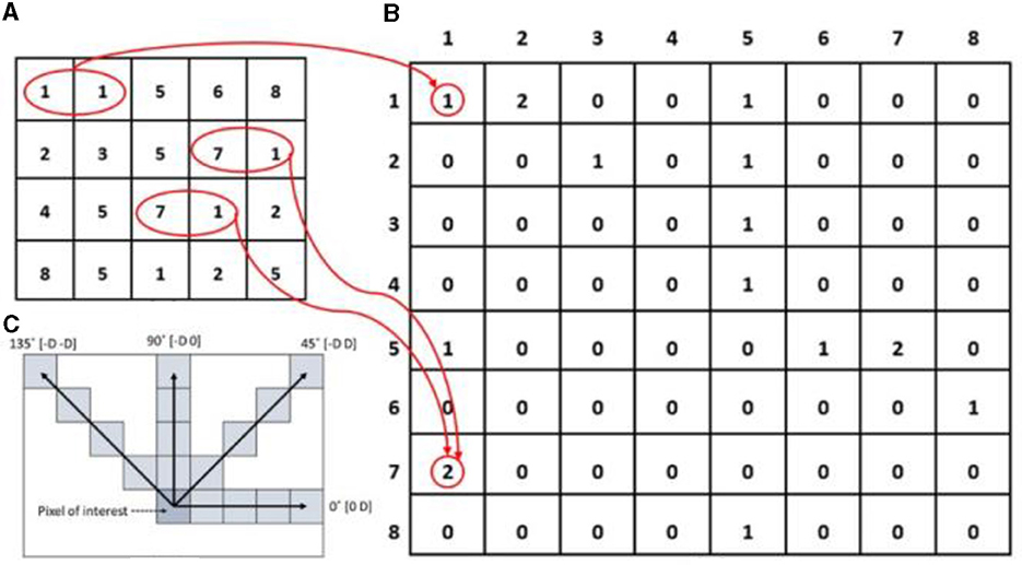
Figure 5. Demonstration of the operational procedure of the Gray Level Co-occurrence Matrix (GLCM) methodology, progressing from the input image (A) to the GLCM image (B). In (C), the spatial connections among pixels are depicted within the array of row-offsets and column-offsets, where 'D' signifies the distance from the pixel of interest. The red circles highlight the frequency with which diverse combinations of gray levels co-occur in the input image, while arrows represent the count of co-occurrences in the GLCM image.

The function f_{(q, r)} represents the intensity value of the pixel at position (q, r) in an image with dimensions (m x n). The four features are described as follows, assuming that P□ [ → ⊺0 (k1, k2)] represents the Gray-Level Co-occurrence Matrix (GLCM) of the image I (q, r) within the region IB. This matrix, for an offset vector o, records the co-occurrence count of intensity pairings (k1, k2).

Feature (S): This feature assesses the degree of similarity between adjacent pixels within a specific area of an image. Equation (9) provides the correlation:

$\begin{array}{ll}S={\sum }_{k_1.k_2}\frac{(k_1-{\mu }_{k_1})(k_2-{\mu }_{k_2})\times P_{\vec{o}}(k_1,k_2)}{{\sigma }_{k1}{\sigma }_{k_2}}& (9)\end{array}$

Contrast (C): The image's contrast value is determined by the abrupt variations in intensity values. It is computed using Equation (10) as follows:

$\begin{array}{ll}C={\sum }_{k_1,k_2}|k_1-k_2{|}^2\times P_{\vec{o}}(k_1,k_2)& (10)\end{array}$

Continuity (C): The homogeneity metric is rooted in the proximity of the GLCM diagonal to the distribution of GLCM elements. It quantifies the degree of similarity or uniformity among pixel intensities. Equation (11) is employed to compute the homogeneity value.

$\begin{array}{ll}H={\sum }_{k_1{k}_2}\frac{P_{\vec{o}}(k_1,k_2)}{1+|k_1-k_2|}& (11)\end{array}$

Energy (E) is defined as the sum of squared elements within the GLCM framework. In the GLCM, a lower energy value indicates a more concentrated or clustered distribution of elements, while a higher energy value signifies a more dispersed distribution. Equation (12) represents the formula for calculating energy:

$\begin{array}{ll}E={\sum }_{k_1,k_2}{P}_{\vec{o}}{(k_1,k_2)}^2& (12)\end{array}$

As mentioned earlier, we calculate four distinct features—Contrast, Homogeneity, Correlation, and Energy—for each of the four offsets. These features sum up to a total of 16 components, constituting the feature vector F(V1) employed for object classification.

2.3.2 The computation of the feature vector F(V2) using wavelets

The Fourier transform serves as a valuable tool in image processing for capturing frequency domain data. By dissecting an image into its sine and cosine components, it reveals the intricate relationship between features in the frequency domain and those in the spatial domain. Through this method, a diverse range of spectral texture patterns with varying densities is unveiled, enabling the extraction of discriminative texture information from transformed images. The Fourier transform is commonly applied in the polar coordinate system (r, θ), where “r” represents the image's intensity, and “θ” denotes its direction.

In contrast, wavelet-based texture analysis employs multiresolution analysis to address the challenge of representing textures at various scales. This approach has been extensively investigated in the realm of texture studies and excels in capturing texture similarities across different scales. The primary advantage of wavelet decomposition lies in its ability to preserve directional selectivity while performing multiscale data analysis. Wavelets, as mathematical operations, segregate data into multiple frequency components, allowing for the examination of each component with a resolution appropriate to its scale.

Wavelets have evolved into powerful mathematical tools for deciphering complex datasets. Wavelet functions exhibit spatial localization, a feature lacking in the Fourier transform, which solely relies on frequency content. While the Fourier transform dissects a signal into a spectrum of frequencies, wavelet analysis dissects it into a hierarchy of scales, ranging from coarsest to finest resolutions. Consequently, wavelet transformation provides a multi-resolution representation of an image, rendering it a superior tool for feature extraction from images.

The Discrete Wavelet Transform (DWT) enables the extraction of diagonal information by decomposing an image into two separate components, namely 0 and 90°. However, the orientations “+45°” and “−45°” are combined and indistinguishable. Moreover, alterations in the input signal can result in significant DWT coefficient variations. To overcome these limitations and enhance directional selectivity, Kingsbury proposed a solution known as the analytic wavelet transform. Another recent development, the dual-tree complex wavelet transform (DT-CWT), exhibits a robust shift-invariance characteristic. Researchers have extensively explored this property of complex wavelets and compared it to the DWT. In contrast to the DWT, the DT-CWT offers superior directional selectivity, distinguishing between six different orientations on a 2D plane: +15°, +45°, +75°,−75°,−45°, and −15°. This enhanced directional selectivity proves particularly beneficial for texture analysis, allowing for functional characterization of textures and simplifying orientation estimation in directional patterns.

The Discrete Wavelet Transform (DWT), an extremely efficient wavelet transform implementation, has now become the method of choice for image analysis. It offers efficient computation and straightforward implementation, rendering it a potent mathematical tool for feature extraction. Its ability to provide simultaneous information regarding the frequency and time localization of image features stands out as one of its key advantages, making it highly valuable for classification tasks. The DWT allows for the extraction of valuable image attributes with reduced computation time and without adding complexity to the implementation.

In the continuous Wavelet Transform (WT), the square-integrable function (t) is employed, and it is mathematically defined by Equations (13) and (14):

$\begin{array}{ll}\begin{array}{l}{W}_v(a,b)={\displaystyle {\int }_{-\alpha }^u\chi (t)y{v}_{a,b}(t)dt}\hfill \end{array}& (13)\end{array}$

$\begin{array}{ll}{\psi }_{\alpha ,b}(t)=\frac{1}{\sqrt{2}}\psi (\frac{t-a}{b})& (14)\end{array}$

The wavelet function (t) is derived from the mother wavelet (t) using two distinct methods: dilation and translation, with scale factor “a” and translation factor “b,” respectively. The 2D Discrete Wavelet Transform (DWT) is employed to decompose the image, as illustrated in the diagram below. The low and high coefficient filters are denoted by the functions g (n) and h (n), respectively. At each level of the transformation, the DWT yields four sub-bands (LL, LH, HL, HH). Figure 6 presents a schematic diagram depicting the 2D DWT process.

FIGURE 6

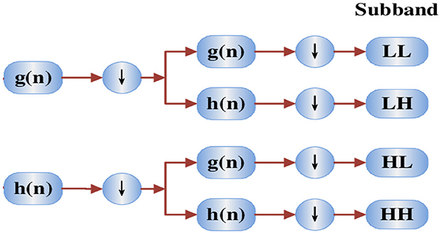
Figure 6. 2D DWT schematic diagram.

2.3.3 Feature vector F(V3) is calculated using Gabor filters

A Gabor filter is a specialized filter designed as a bandpass filter, capable of detecting various orientations. Its distinctive structure allows it to be responsive to rotations, effectively capturing a wide range of orientations. To ensure robustness to rotation, a commonly used Gabor filter is circularly symmetric, considering all directions for each passband. The magnitude of the Gabor-filtered image serves as a valuable Gabor feature, indicating the signal strength within the corresponding passband.

Originally, Gabor filters were primarily employed to characterize the textural attributes of an image. Unlike GLCM textures, which rely on pixel relationships, Gabor filters utilize the power spectrum in the frequency domain to compute texture features through a two-step process. Initially, the input image undergoes a transformation into the frequency domain using a Gabor filter to quantify variations in pixel intensities. Subsequently, the image's diverse textures are represented by a range of frequencies and orientations.

In essence, a 2D Gabor filter is akin to a sinusoidal plane wave modulated by a Gaussian kernel, as illustrated in Equation (15):

$\begin{array}{l}{G}_d(x,y\mid \omega ,\theta ,\varphi ,c_x,c_y)=\exp \left(\frac{-\left\{{(x-c_x)}^2-{(y-c_y)}^2\right\}}{2{\sigma }^2}\right)\\ \times \sin (\omega (x\cos \theta -y\sin \theta )+\varphi )& (15)\end{array}$

In the Gabor filter equation, the variable “f” represents frequency, “θ” denotes the filter angle, “φ” represents the phase shift, and “σ” signifies the Gaussian variance. The filter's center is indicated by the values (cx, cy). The Gabor spectrum for an MRI image, denoted as I (x, y), is generated by performing a linear convolution of I GK, which represents the Gabor kernel. In this work, the Gabor spectrum is employed to discern texture features in five different orientations. Only changes in orientation are taken into consideration because MRI images exhibit consistent textural characteristics concerning phase and frequency. These five distinct orientations are employed to align with the five parameters in the CLCM (possibly referring to a separate approach). Equation (16) defines these orientations, denoted as 0, 1, 2, 3, and 4:

$\begin{array}{l}{G}_{K\{1,2,\dots ,5\}}={\displaystyle \sum _{xy}^{S(xy)}{G}_k(x,y/\omega ,\{0,\pi /5\dots ,4\pi /5\},\phi ,c_x,c_y)}\\ \otimes I(x,y)& (16)\end{array}$

When performing convolution between two functions, the convolution operator, symbolized by the symbol, is utilized. In this instance, it is used to compute the MRI image's Gabor texture features. The parameter GK 1, 2,..., 5 corresponds to the Gabor texture characteristics.

2.3.4 Three feature vectors concatenated

The feature vector F(V), which amalgamates the dimensions essential for the ultimate classification of brain tumors, is portrayed as the summation of three constituent feature vectors: F(V1) + F(V2) + F(V3).

2.4 Classification of features

Classification is performed by leveraging spectral or spectrally defined features, encompassing attributes such as density and texture, within the feature space. A decision rule is employed to partition the feature space into distinct classes. The objective of statistical classification is to make predictions based on given inputs. These classification algorithms rely on a training set of attributes and their corresponding outputs, often termed output predictors. By establishing correlations between these attributes, classifier algorithms are equipped to forecast future outcomes.

2.4.1 SVM classification

Support Vector Machines (SVM), a robust supervised machine learning technology, emerged within the framework of statistical learning theory [55, 56]. SVM offers versatile applications, including non-linear regression and noise reduction tasks. Its appeal stems from its ability to generalize effectively to new data, even without prior domain expertise. In SVM's classification process, a discriminative hyperplane that maximizes the margin between classes within the feature space is identified. This hyperplane is found by utilizing labeled training data to estimate a function f_{(x, y)}, enabling it to categorize new instances in the testing set. Various researchers have also achieved noteworthy success by incorporating fuzzy learning approaches into classification across diverse disciplines.

SVM stands as a state-of-the-art classifier in the realm of machine learning, garnering considerable attention in recent years. Initially proposed by Vapnik and Cortes [57] and grounded in statistical learning theory, SVM is renowned for its exceptional generalization capabilities, particularly in high-dimensional feature spaces. The fundamental concept behind SVM involves mapping the input vector x into a higher-dimensional feature space Z through a predefined nonlinear transformation. In this transformed space, an optimal separation hyperplane is constructed. SVM efficiently classifies binary classes for pattern recognition by determining a decision surface defined by crucial data points from the training set, known as support vectors (Equation 17).

In Equation (17), H denotes a hyperplane such that:

$\begin{array}{l}{x}_i.w+b\ge +1when{y}_i=+1\\ and\\ x_I.w+b\le -1when{y}_i=-1& (17)\end{array}$

Within this context, H1 and H2 represent two planes defined by:

H1: x_i.w = +1

H2: x_i.w = −1

The points on the planes H1 and H2 correspond to the support vectors. The distance d+ represents the shortest distance from the nearest positive point on the hyperplane, while the distance d- signifies the shortest distance from the nearest negative point. As depicted in Figure 7, the decision boundary, carefully selected, effectively separates multiple groups.

FIGURE 7

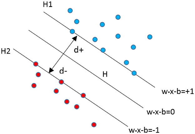
Figure 7. Selection of the decision boundary in SVM classification.

The SVM algorithm employs the vector of multi-model texture features extracted from the MR images as its input. Within the feature space, this input feature dataset is segregated into two distinct groups for the classification task: normal images and abnormal images. Each n-dimensional input, represented as xi (where i ranges from 1 to N), is assigned a label, li, which takes a value of +1 for normal images and −1 for aberrant images. The SVM's decision function, as depicted in Equation (18), furnishes a method for categorizing each input based on these labels.

$\begin{array}{ll}\text{des}(\text{x})=\text{w}.\text{x}+\text{b}& (18)\end{array}$

where b is a scalar, w is an n-dimensional vector, and

$\begin{array}{l}{y}_i=des(x_i)\ge 1fori=1,2,,\dots N.\end{array}$

It is evident from the equations outlined above that during the model training, the trained samples may potentially fall on either side of the hyperplane. The decision is resolved by employing the coefficient vector w to assess the sign of yi.

In the context of brain tumor detection and classification, classifiers utilize Multi-Model Texture Features (MMTFs) as input. SVM proves to be a suitable approach for addressing this binary classification challenge, especially when dealing with discrete data values across a dataset comprising a substantial number of images. The classifier's accuracy is evaluated by comparing the categorized outputs with the ground truth data.

The experiments conducted in this study employ the publicly accessible implementation library, LibSVM. The choice of the radial basis function (RBF) kernel is based on its superior performance in cross-validation compared to other kernel options. To determine the optimal values for the SVM kernel's parameters, namely C and gamma, a grid search approach is employed.

2.4.2 LS-SVM: short for Least Squares Support Vector Machine

The Least Squares Support Vector Machine (LS-SVM) augments the standard Support Vector Machine (SVM) framework [58]. It introduces a shift from the conventional inequality constraints to equality constraints and employs the sum of squared error loss function as a measure of the training set's empirical loss. This transformation allows the quadratic programming problem to be reformulated into a more manageable linear equation problem. LS-SVM exhibits superior performance compared to SVM, excelling in both solution speed and accuracy. The choice of the LS-SVM in our brain tumor classification system is grounded in its ability to deliver superior generalization performance, handle non-linear data patterns, provide a sparse and interpretable solution, and maintain robustness to overfitting. Its adaptability to diverse dataset sizes and strong theoretical foundation make it a well-suited method for the complex task of classifying brain tumors in MRI images, ensuring high accuracy and trustworthiness in the medical field.

The LS-SVM can be succinctly elucidated in the ensuing sections. In the training dataset, the input vector xi and its corresponding target vector yi are denoted as xi, yi (where i ranges from 1 to l). The mapping of the input space to a higher-dimensional feature space through the mapping function U results in the feature space vector zi, or pi(xi). Consequently, the hyperplane is described by the equation in Equation (19).

$\begin{array}{ll}\text{w}.\text{z}+\text{b}=0& (19)\end{array}$

Here, the weight vector w determines the hyperplane's orientation, while the bias parameter b influences its position. For efficient computations, LS-SVM aims to minimize the following objective function:

$\begin{array}{l}\text{Reduce}:J(w,e)=\frac{1}{2}{w}^{T}w+\frac{1}{2}C{\displaystyle \sum _{i=1}^N}{e}_i^2\end{array}$

where i is a positive integer between 1 and N.

There must be a (w, b) such that the following stipulation holds for data samples to be regarded as linearly separable:

In accordance with $y_i=w^T{z}_i+b+e_{i}i=1,2,\dots .N$

Equation (20) defines the Lagrange equation.

$\begin{array}{ll}L(w,b,e,\alpha )=J(w,e)-{\displaystyle \sum _{i=1}^N}{\alpha }_i\left\{w^T{z}_i+b+e_i-y_i\right\}& (20)\end{array}$

The optimality criterion for Lagrange multipliers are as follows: $\frac{\partial L}{\partial w}=0,\frac{\partial L}{\partial b}=0,\frac{\partial L}{\partial e_i}=0,and\frac{\partial L}{\partial {\alpha }_i}$ are obtained when w and e are removed.

$\left[\begin{array}{c}01_v^T\\ 1_v\Omega +\frac{I}{C}\end{array}\right]\left[\begin{array}{c}b\\ \alpha \end{array}\right]=\left[\begin{array}{c}0\\ y\end{array}\right]$

Where

$\begin{array}{l}y={\left[y_1,y_2,y_3,\dots \dots y_N\right]}^T,1_v={\left[1,11,\dots \dots 1\right]}^T,\\ \alpha ={\left[{\alpha }_1,{\alpha }_2,{\alpha }_3,\dots .{\alpha }_N\right]}^T\end{array}$

And Ω_{i, j} = K(x_i, x_j), for i, j = 1, 2, 3, ……N

The kernel function of the Radial Basis Function (RBF) is denoted by

$\begin{array}{l}K(x_i,x_j)=e^{\left[\frac{-{x|x_i-x_j|}^2}{{\sigma }^2}\right]}\end{array}$

The spread or width of the kernel is determined by the parameter mentioned above. The characteristics of the smooth fitting function in the equation are influenced significantly by the selection of the kernel function.

2.5 Dataset description

The experimental dataset comprises a total of 259 brain MRI scans, with 50 categorized as normal and the remaining 209 as aberrant. These images were sourced from the Kaggle data archive and were acquired using a SIEMENS 1.5 Tesla MR device. The imaging settings included a matrix size of 256 x 256, a slice thickness of 1 mm, and the acquisition of T1-weighted post-contrast (Gadolinium) images using a Spin-Echo (SE) sequence with a repetition time (TR) of 480 ms and an echo time (TE) of 8.7 ms.

The classification system employed in this study consists of two phases: training and testing. For the training phase, a subset of 30 normal images and 90 aberrant images was utilized. The remaining 139 images, comprising 20 normal and 119 abnormal scans, were reserved for testing. Figure 8 showcases representative examples of both normal and aberrant T1-weighted MRI scans from the dataset.

FIGURE 8

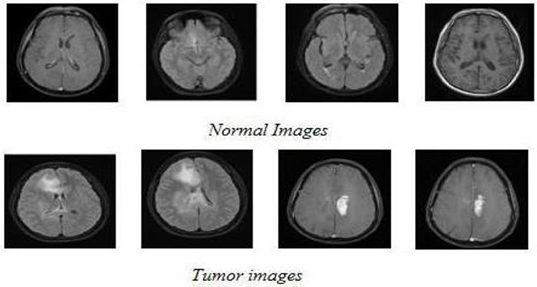
Figure 8. Actual T1w MRI scans that are normal and abnormal.

2.6 Experimental environment settings and performance evaluation metrics

This research aims to propose an optimal model which identifies and classifies different types of images. The proposed model was implemented using Python (v. 3.8), OpenCV (v. 4.7), Keras Library (v. 2.8) were used on Windows 10 Pro OS, with system configuration using an Intel i5 processor running at 2.9 GHz, an Nvidia RTX 2060 Graphical Processing Unit and 16 GB RAM.

Sensitivity (Sen), specificity (Spe), and accuracy (Pre) are three commonly employed benchmark metrics for assessing the reliability of the experimental results. These metrics were derived from the analysis of the confusion matrix, as presented in Table 1.

TABLE 1

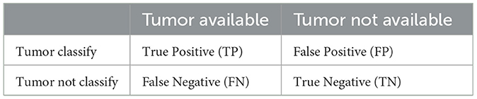
Table 1. Confusion matrix of TP, TN, FP, and FN.

From the Table, the variables TP, FP, TN, and FN correspond to the proportions of true positives, false positives, true negatives, and false negatives, respectively. Sensitivity, often referred to as the true positive rate (TPR), is defined as the ratio of true positives to the sum of false negatives and true positives, as expressed in Equation (21).

$\begin{array}{ll}\text{Sen}=\text{TP}/(\text{TP}+\text{FN})& (21)\end{array}$

From the data available in the confusion matrix, specificity, also known as the false positive rate (FPR), can be computed. It quantifies the ratio of false positives to the sum of true negatives and false positives, as demonstrated in Equation (22):

$\begin{array}{ll}\text{Spe}=\text{TN}/(\text{TN}+\text{FP})& (22)\end{array}$

Accuracy, on the other hand, measures the extent to which the results of a classification algorithm align with real-world outcomes. It is calculated as the ratio of correct predictions to the total number of predictions made, as defined in Equation (23):

$\begin{array}{ll}\text{Accuracy}=(\text{TN}+\text{TP})/(\text{TotalPixels})& (23)\end{array}$

The categorization error rate is determined using the formula provided in Equation (24):

$\begin{array}{ll}\text{Error rate}=1-\text{Accuracy}& (24)\end{array}$

3 Results

The conducted experiments represent a meticulous effort to identify the most suitable classifier for our proposed regional classification pipeline. These findings are pivotal in the development of an effective and reliable approach for classifying brain regions in MRI scans. Below, we provide a comprehensive analysis of the results, highlighting key takeaways, strengths, and significant insights.

3.1 Diverse classifier evaluation

The experimentation process involved a comprehensive examination of a variety of neural network-based classifiers, including Support Vector Machines (SVM), Radial Basis Function (RBF), Artificial Neural Networks (ANN), and Least Squares Support Vector Machines (LS-SVM). This diversity in classifier selection allowed for a robust assessment of their performance across various dimensions.

3.2 Quantitative and qualitative assessments

To ensure a well-rounded evaluation, both quantitative and qualitative assessments were employed. This approach allowed for a comprehensive understanding of how each classifier performed, considering a range of metrics and visual representations.

Table 2 provides a detailed breakdown of performance metrics for each classifier, offering insights into their ability to correctly classify brain regions. Notably, these metrics include True Positives (TP), True Negatives (TN), False Positives (FP), False Negatives (FN), Sensitivity, Specificity, and Accuracy. These metrics are essential for assessing a classifier's overall performance. These details are also represented in Figure 9.

TABLE 2

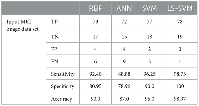
Table 2. Lists the outcomes of the proposed MMTF's classification using several classifier techniques on the testing dataset.

FIGURE 9

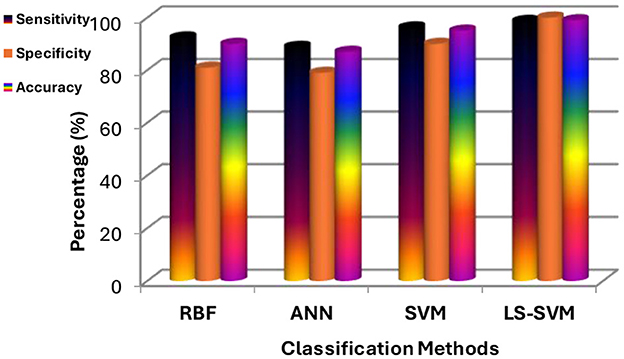
Figure 9. Results of experiments using the proposed MMTF and different classifiers (LS-SVM, RBF, SVM, and ANN).

Key Findings and Strengths:

1. LS-SVM dominance: the standout result from the experimentation is the remarkable performance of LS-SVM. When compared to other classifiers, LS-SVM consistently outperforms them in terms of accuracy, sensitivity, specificity, and error rate. This indicates its exceptional ability to accurately classify brain regions in MRI scans.

2. Accuracy and error rate: LS-SVM achieves an accuracy of 98.97% and an impressively low error rate of 0.01%. These metrics reflect LS-SVM's proficiency in making accurate classifications, which is of paramount importance in medical image analysis.

3. False negatives: LS-SVM also excels in minimizing false negatives, signifying its capability to avoid missing relevant regions. This is crucial in medical applications, where missing abnormalities can have serious consequences.

4. Qualitative insights: beyond numbers and metrics, the qualitative evaluation allowed for a nuanced assessment of how each classifier performed in practice. This insight is valuable in real-world applications.

The Table 3 offers a concise summary of the performance metrics of four distinct classifiers: Radial Basis Function (RBF), Artificial Neural Networks (ANN), Support Vector Machines (SVM), and Least Squares Support Vector Machines (LS-SVM). The metrics include False Positives (FP), False Negatives (FN), Accuracy, and Error Rate. These details are also represented in Figure 10.

TABLE 3

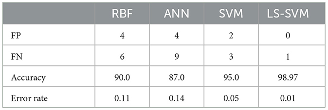
Table 3. Performance metrics of different classifiers.

FIGURE 10

Figure 10. FP, FN, accuracy and error rate of different classifiers.

According to the Table 3, the analysis of performance metrics for different classifiers provides valuable insights into their respective capabilities in classifying brain regions in MRI scans. False Positives (FP) represent instances incorrectly classified as positive when they are actually negative. In this regard, LS-SVM stands out remarkably by achieving zero False Positives, signifying its precision and the absence of misclassifications. SVM and RBF also perform well with a small number of False Positives (2 and 4, respectively), but LS-SVM's performance in this aspect is superior. ANN, with 4 False Positives, aligns closely with SVM and RBF but lags behind LS-SVM.

On the other hand, False Negatives (FN), indicating instances incorrectly classified as negative when they are actually positive, are crucial in medical applications where missing abnormalities can lead to delayed diagnoses. LS-SVM excels with just 1 False Negative, demonstrating its heightened sensitivity to detecting positive instances. SVM and RBF perform well in this respect with 3 and 6 False Negatives, respectively, while ANN's 9 False Negatives indicate its relative weakness in identifying positive instances.

Accuracy, which represents the overall proportion of correctly classified instances, is notably higher for LS-SVM at 98.97%, showcasing its superiority in correctly classifying brain regions in MRI scans. SVM follows closely with an accuracy of 95.0%, while RBF and ANN achieve lower accuracy scores at 90.0 and 87.0%, respectively. These results highlight LS-SVM's exceptional accuracy in comparison to the other classifiers.

The error rate, measuring the proportion of misclassified instances, is significantly lower for LS-SVM at 0.01%, indicating the classifier's precision and reliability. SVM also demonstrates a low error rate at 0.05%, affirming its ability to classify brain regions accurately. In contrast, RBF and ANN have higher error rates at 0.11 and 0.14, respectively, suggesting a comparatively higher level of misclassification.

The analysis of performance metrics for different classifiers in our brain region classification study reveals critical insights into the capabilities and effectiveness of each method. These findings are instrumental in understanding the nuances of classifier performance, with a particular focus on their abilities to accurately classify brain regions in MRI scans. Among the classifiers examined, one stands out as the clear frontrunner: the (LS-SVM). With exceptional dominance in multiple aspects, including False Positives, False Negatives, accuracy, and error rate, LS-SVM emerges as a powerful and precise tool in the field of medical imaging. This section delves into the key findings and strengths derived from our comprehensive analysis, emphasizing the significance of LS-SVM as a valuable asset in enhancing the accuracy of brain tumor diagnosis.

Key Findings and Strengths:

• LS-SVM Dominance: The most prominent and consistent finding in the analysis is the exceptional performance of the LS-SVM classifier. It excels in several crucial aspects, including minimizing False Positives, False Negatives, accuracy, and error rate. This dominance signifies its reliability and precision in accurately classifying brain regions in MRI scans, making it a standout choice for this critical task.

• Zero False Positives: LS-SVM achieves the remarkable feat of having zero False Positives, which means it does not misclassify any negative instances as positive. This zero tolerance for false alarms is crucial in medical applications, as it significantly reduces the risk of unnecessary interventions and incorrect diagnoses.

• Minimized False Negatives: LS-SVM's capacity to minimize False Negatives, with only one instance, underscores its exceptional sensitivity to detecting positive instances. This capability is of utmost importance in medical imaging, where missing abnormalities can lead to delayed or overlooked diagnoses, with potentially severe consequences.

• Exceptional Accuracy: LS-SVM achieves the highest accuracy among all classifiers, at 98.97%. This extraordinary accuracy reflects its ability to correctly classify brain regions, highlighting its importance in precision medical image analysis, where accurate results are critical.

• Low Error Rate: LS-SVM boasts the lowest error rate of 0.01%, signifying its precision and reliability in classifying brain regions. A low error rate is pivotal in medical applications, where misclassifications can have severe implications for patient care and diagnosis.

• SVM's Strong Performance: While LS-SVM outperforms all other classifiers, it is essential to recognize the strong performance of SVM, which achieves a high accuracy and low error rate. This strength makes SVM a credible alternative in cases where the specific advantages of LS-SVM may not be required.

4 Conclusion

Our investigation has propelled the domain of brain tumor classification in MRI imaging by introducing a groundbreaking methodology that integrates Least Squares Support Vector Machines (LS-SVM) with Multi-Scale Morphological Texture Features (MMTF) extracted from T1-weighted MR images. The comprehensive assessment conducted on a substantial dataset comprising 139 cases, including both abnormal and normal brain images, has unequivocally showcased the unparalleled performance of LS-SVM, surpassing established classifiers like SVM, RBF, and ANN. This achievement stands as a hallmark, boasting an extraordinary accuracy rate of 98.97%, coupled with an exceptional reduction in misclassifications, evidenced by zero False Positives and minimal False Negatives. The clinical implications are substantial, promising enhanced diagnostic precision and sensitivity to abnormalities in brain tumor identification, which directly impacts and elevates the standard of care in medical imaging and radiology.

Our research not only advances the immediate clinical application of precise brain tumor classification but also contributes significantly to the scientific understanding of classifier methodologies in medical imaging. The exceptional performance of LS-SVM sets a new benchmark, offering heightened accuracy, reduced misclassifications, and substantial scientific insights into classifier capabilities in medical diagnostics. Moreover, the limitations of our study, chiefly the reliance on a relatively confined dataset, necessitate future exploration using more extensive and varied data to validate and generalize LS-SVM's applicability in diverse clinical settings. Additionally, further investigation into the interpretability of LS-SVM's classifications would augment its practical utility in clinical scenarios, supporting radiologists in comprehending and trusting the automated diagnostic process.

The findings from our research hold transformative potential for immediate and future applications in clinical settings. LS-SVM's exceptional accuracy and reliability in classifying brain regions in MRI scans, along with the scientific insights derived from our analysis, pave the way for the development of more reliable and precise diagnostic tools in medical imaging. In summary, our investigation significantly advances brain tumor classification methodologies, highlighting LS-SVM's unprecedented accuracy and reliability. This breakthrough offers a promising avenue for reshaping and improving brain tumor diagnosis, providing a more dependable and precise tool for radiologists and healthcare professionals.

Future research endeavors could significantly expand on this study by encompassing larger, more diverse datasets to further validate and generalize the robustness of LS-SVM in varied clinical settings. Additionally, delving into the interpretability and explainability of LS-SVM's classifications could substantially enhance its practical applicability in clinical scenarios, aiding radiologists in comprehending and trusting the automated diagnostic process. Exploring the integration of advanced imaging modalities or incorporating additional features, such as dynamic or functional imaging parameters, could broaden the scope of this research, potentially leading to more comprehensive and accurate diagnostic tools. Furthermore, investigating the adaptability of this methodology to real-time or longitudinal imaging data could fortify its applicability in ongoing monitoring and treatment evaluation for brain tumor patients. These future directions hold promise for refining and expanding the application of LS-SVM in medical imaging and strengthening its role in precise and reliable brain tumor classification.

Data availability statement

The original contributions presented in the study are included in the article/supplementary material, further inquiries can be directed to the corresponding authors.

Author contributions

FK: Conceptualization, Investigation, Methodology, Writing—original draft, Writing—review & editing. YG: Conceptualization, Data curation, Formal analysis, Funding acquisition, Investigation, Methodology, Project administration, Resources, Software, Supervision, Validation, Visualization, Writing—original draft, Writing—review & editing. SA: Conceptualization, Data curation, Formal analysis, Investigation, Methodology, Software, Writing—original draft, Writing—review & editing. MM: Conceptualization, Data curation, Investigation, Methodology, Writing—review & editing. MSM: Conceptualization, Investigation, Methodology, Writing—review & editing. AS: Methodology, Writing—review & editing.

Funding

The author(s) declare financial support was received for the research, authorship, and/or publication of this article. This work was supported by the Deanship of Scientific Research, Vice Presidency for Graduate Studies and Scientific Research, King Faisal University, Saudi Arabia, under the Project GRANT5,124.

Conflict of interest

The authors declare that the research was conducted in the absence of any commercial or financial relationships that could be construed as a potential conflict of interest.

Publisher's note

All claims expressed in this article are solely those of the authors and do not necessarily represent those of their affiliated organizations, or those of the publisher, the editors and the reviewers. Any product that may be evaluated in this article, or claim that may be made by its manufacturer, is not guaranteed or endorsed by the publisher.

References

1. The Brain Tumor Charity. Brain Tumor Basics. Available online at: https://www.thebraintumourcharity.org/ (accessed August 22, 2023).

Google Scholar

2. Louis DN, Perry A, Wesseling P, Brat DJ, Cree IA, Figarella-Branger D, et al. The 2021 WHO classification of tumors of the central nervous system: a summary. Neuro Oncol. (2021) 23:1231–51. doi: 10.1093/neuonc/noab106

CrossRef Full Text | Google Scholar

3. Tandel GS, Biswas M, Kakde OG, Tiwari A, Suri HS, Turk M, et al. A review on a deep learning perspective in brain cancer classification. Cancers. (2019) 11:111. doi: 10.3390/cancers11010111

PubMed Abstract | CrossRef Full Text | Google Scholar

4. Tamimi AF, Juweid M. Epidemiology and outcome of glioblastoma. Glioblastoma. (2017) 143–53. doi: 10.15586/codon.glioblastoma.2017.ch8

CrossRef Full Text | Google Scholar

5. Dhiman P, Bonkra A, Kaur A, Gulzar Y, Hamid Y, Mir MS, et al. Healthcare trust evolution with explainable artificial intelligence: bibliometric analysis. Information. (2023) 14:541. doi: 10.3390/info14100541

CrossRef Full Text | Google Scholar

6. Gordillo N, Montseny E, Sobrevilla P. State of the art survey on MRI brain tumor segmentation. Magn Reson Imaging. (2013) 31:1426–38. doi: 10.1016/j.mri.2013.05.002

PubMed Abstract | CrossRef Full Text | Google Scholar

7. Khan F, Ayoub S, Gulzar Y, Majid M, Reegu FA, Mir MS, et al. MRI-based effective ensemble frameworks for predicting human brain tumor. J Imaging. (2023) 9:163. doi: 10.3390/jimaging9080163

PubMed Abstract | CrossRef Full Text | Google Scholar

8. Anand V, Gupta S, Gupta D, Gulzar Y, Xin Q, Juneja S, et al. Weighted average ensemble deep learning model for stratification of brain tumor in MRI images. Diagnostics. (2023) 13:1320. doi: 10.3390/diagnostics13071320

PubMed Abstract | CrossRef Full Text | Google Scholar

9. Mabray MC, Ramon F, Barajas J, Cha S. Modern brain tumor imaging. Brain Tumor Res Treat. (2015) 3:8–23. doi: 10.14791/btrt.2015.3.1.8

CrossRef Full Text | Google Scholar

10. Holland EC. Gliomagenesis: genetic alterations and mouse models. Nat Rev Genet. (2001) 2:120–9. doi: 10.1038/35052535

PubMed Abstract | CrossRef Full Text | Google Scholar

11. Villanueva-Meyer JE, Mabray MC, Cha S. Current clinical brain tumor imaging. Neurosurgery. (2017) 81:397. doi: 10.1093/neuros/nyx103

PubMed Abstract | CrossRef Full Text | Google Scholar

12. Siyoum Biratu E, Schwenker F, Ayano YM, Debelee TG, Militello C, Conti V, et al. Survey of brain tumor segmentation and classification algorithms. J Imaging. (2021) 7:179. doi: 10.3390/jimaging7090179

PubMed Abstract | CrossRef Full Text | Google Scholar

13. Zaccagna F, Grist JT, Quartuccio N, Riemer F, Fraioli F, Caracò C, et al. Imaging and treatment of brain tumors through molecular targeting: recent clinical advances. Eur J Radiol. (2021) 142:109842. doi: 10.1016/j.ejrad.2021.109842

PubMed Abstract | CrossRef Full Text | Google Scholar

14. Khan H, Shah PM, Shah MA, ul Islam S, Rodrigues JJPC. Cascading handcrafted features and convolutional neural network for IoT-enabled brain tumor segmentation. Comput Commun. (2020) 153:196–207. doi: 10.1016/j.comcom.2020.01.013

CrossRef Full Text | Google Scholar

15. Mehmood A, Gulzar Y, Ilyas QM, Jabbari A, Ahmad M, Iqbal S. SBXception: A shallower and broader Xception architecture for efficient classification of skin lesions. Cancers. (2023) 15:3604. doi: 10.3390/cancers15143604

PubMed Abstract | CrossRef Full Text | Google Scholar

16. Majid M, Gulzar Y, Ayoub S, Khan F, Reegu FA, Mir MS, et al. Enhanced transfer learning strategies for effective kidney tumor classification with CT imaging. Int J Adv Comput Sci Appl. (2023) 14:2023. doi: 10.14569/IJACSA.2023.0140847

CrossRef Full Text | Google Scholar

17. Pluim JPW, Maintz JBA, Viergever MA. Multiscale approach to mutual information matching. Proc Med Imaging. (1998) 3338:1334–44. doi: 10.1117/12.310862

CrossRef Full Text | Google Scholar

18. Sahlan F, Hamidi F, Misrat MZ, Adli MH, Wani S, Gulzar Y. Prediction of mental health among university students. Int J Percept Cogn Comput. (2021) 7:85–91. Available online at: https://journals.iium.edu.my/kict/index.php/IJPCC/article/view/225

Google Scholar

19. Hanafi MFFM, Nasir MSFM, Wani S, Abdulghafor RAA, Gulzar Y, Hamid Y. A real time deep learning based driver monitoring system. Int J Percept Cogn Comput. (2021) 7:79–84. Available online at: https://journals.iium.edu.my/kict/index.php/IJPCC/article/view/224

Google Scholar

20. Gulzar Y, Alwan AA, Abdullah RM, Abualkishik AZ, Oumrani M. OCA: ordered clustering-based algorithm for E-commerce recommendation system. Sustainability. (2023) 15:2947. doi: 10.3390/su15042947

CrossRef Full Text | Google Scholar

21. Gulzar Y, Ünal Z, Aktas HA, Mir MS. Harnessing the power of transfer learning in sunflower disease detection: a comparative study. Agriculture. (2023) 13:1479. doi: 10.3390/agriculture13081479

CrossRef Full Text | Google Scholar

22. Dhiman P, Kaur A, Balasaraswathi VR, Gulzar Y, Alwan AA, Hamid Y. Image acquisition, preprocessing and classification of citrus fruit diseases: a systematic literature review. Sustainability. (2023) 15:9643. doi: 10.3390/su15129643

CrossRef Full Text | Google Scholar

23. Gulzar Y. Fruit image classification model based on mobileNetV2 with deep transfer learning technique. Sustainability. (2023) 15:1906. doi: 10.3390/su15031906

CrossRef Full Text | Google Scholar

24. Mamat N, Othman MF, Abdulghafor R, Alwan AA, Gulzar Y. Enhancing image annotation technique of fruit classification using a deep learning approach. Sustainability. (2023) 15:901. doi: 10.3390/su15020901

CrossRef Full Text | Google Scholar

25. Gulzar Y, Hamid Y, Soomro AB, Alwan AA, Journaux LA. Convolution neural network-based seed classification system. Symmetry. (2020) 12:2018. doi: 10.3390/sym12122018

CrossRef Full Text | Google Scholar

26. Malik I, Ahmed M, Gulzar Y, Baba SH, Mir MS, Soomro AB, et al. Estimation of the extent of the vulnerability of agriculture to climate change using analytical and deep-learning methods: a case study in Jammu, Kashmir, and Ladakh. Sustainability. (2023) 15:11465. doi: 10.3390/su151411465

CrossRef Full Text | Google Scholar

27. Khan SA, Gulzar Y, Turaev S, Peng YS. A Modified HSIFT descriptor for medical image classification of anatomy objects. Symmetry. (2021) 13:1987. doi: 10.3390/sym13111987

CrossRef Full Text | Google Scholar

28. Alam S, Raja P, Gulzar Y. Investigation of machine learning methods for early prediction of neurodevelopmental disorders in children. Wireless Commun Mob Comput. (2022) 2022:1-12. doi: 10.1155/2022/5766386

CrossRef Full Text | Google Scholar

29. Ayoub S, Gulzar Y, Rustamov J, Jabbari A, Reegu FA, Turaev S. Adversarial approaches to tackle imbalanced data in machine learning. Sustainability. (2023) 15:7097. doi: 10.3390/su15097097

CrossRef Full Text | Google Scholar

30. Hamid Y, Elyassami S, Gulzar Y, Balasaraswathi VR, Habuza T, Wani S. An improvised CNN model for fake image detection. Int J Inform Technol. (2022) 2022:1–11. doi: 10.1007/s41870-022-01130-5

CrossRef Full Text | Google Scholar

31. Aggarwal S, Gupta S, Gupta D, Gulzar Y, Juneja S, Alwan AA, et al. An artificial intelligence-based stacked ensemble approach for prediction of protein subcellular localization in confocal microscopy images. Sustainability. (2023) 15:1695. doi: 10.3390/su15021695

CrossRef Full Text | Google Scholar

32. Albarrak K, Gulzar Y, Hamid Y, Mehmood A, Soomro AB. A deep learning-based model for date fruit classification. Sustainability. (2022) 14:6339. doi: 10.3390/su14106339

CrossRef Full Text | Google Scholar

33. Hamid Y, Wani S, Soomro AB, Alwan AA, Gulzar Y. Smart seed classification system based on mobileNetV2 architecture. In Proceedings of the 2022 2nd International Conference on Computing and Information Technology (ICCIT) (Tabuk) (2022). p. 217–22. doi: 10.1109/ICCIT52419.2022.9711662

CrossRef Full Text | Google Scholar

34. Siar M, Teshnehlab M. Brain tumor detection using deep neural network and machine learning algorithm. In: Proceedings of the 2019 9th International Conference on Computer and Knowledge Engineering, ICCKE (Mashhad) (2019). doi: 10.1109/ICCKE48569.2019.8964846

CrossRef Full Text | Google Scholar

35. Bonnici V, Cicceri G, Distefano S, Galletta L, Polignano M, Scaffidi C. Covid19/IT the digital side of COVID19: a picture from italy with clustering and taxonomy. PLoS ONE. (2022) 17:e0269687. doi: 10.1371/journal.pone.0269687

PubMed Abstract | CrossRef Full Text | Google Scholar

36. Seetha J, Raja SS. Brain tumor classification using convolutional neural networks. Biomed Pharmacol J. (2018) 11:1457–61. doi: 10.13005/bpj/1511

CrossRef Full Text | Google Scholar

37. Gupta D, Richhariya B. Entropy based fuzzy least squares twin support vector machine for class imbalance learning. Appl Intell. (2018) 48:4212–31. doi: 10.1007/s10489-018-1204-4

CrossRef Full Text | Google Scholar

38. Hazarika BB, Gupta D, Borah P. Fuzzy twin support vector machine based on affinity and class probability for class imbalance learning. Knowl Inf Syst. (2023) 65:5259–88. doi: 10.1007/s10115-023-01904-8

CrossRef Full Text | Google Scholar

39. Gulzar Y, Khan SA. (Skin lesion segmentation based on vision transformers and convolutional neural networks—a comparative study. Appl Sci. (2022) 12:5990. doi: 10.3390/app12125990

CrossRef Full Text | Google Scholar

40. Ayoub S, Gulzar Y, Reegu FA, Turaev S. Generating image captions using bahdanau attention mechanism and transfer learning. Symmetry. (2022) 14:2681. doi: 10.3390/sym14122681

CrossRef Full Text | Google Scholar

41. Cirrincione G, Cannata S, Cicceri G, Prinzi F, Currieri T, Lovino M, et al. Transformer-based approach to melanoma detection. Sensors. (2023) 23:5677. doi: 10.3390/s23125677

PubMed Abstract | CrossRef Full Text | Google Scholar

42. Bektas B, Emre IE, Kartal E, Gulsecen S. Classification of mammography images by machine learning techniques. In: UBMK 2018 - 3rd International Conference on Computer Science and Engineering (Sarajevo) (2018). p. 580–5. doi: 10.1109/UBMK.2018.8566380

CrossRef Full Text | Google Scholar

43. Saeedi S, Rezayi S, Keshavarz H, Niakan Kalhori RS. MRI-based brain tumor detection using convolutional deep learning methods and chosen machine learning techniques. BMC Med Inform Decis Mak. (2023) 23:16. doi: 10.1186/s12911-023-02114-6

PubMed Abstract | CrossRef Full Text | Google Scholar

44. Sharma AK, Nandal A, Dhaka A, Zhou L, Alhudhaif A, Alenezi F, et al. Brain tumor classification using the modified resnet50 model based on transfer learning. Biomed Signal Process Control. (2023) 86:105299. doi: 10.1016/j.bspc.2023.105299

CrossRef Full Text | Google Scholar

45. Qin C, Li B, Han B. Fast brain tumor detection using adaptive stochastic gradient descent on shared-memory parallel environment. Eng Appl Artif Intell. (2023) 120:105816. doi: 10.1016/j.engappai.2022.105816

CrossRef Full Text | Google Scholar

46. Mathew AR, Anto PB. Tumor detection and classification of MRI brain image using wavelet transform and SVM. In: Proceedings of the Proceedings of IEEE International Conference on Signal Processing and Communication, ICSPC 2017 (Coimbatore). (2018). doi: 10.1109/CSPC.2017.8305810

CrossRef Full Text | Google Scholar

47. Zulfiqar F, Ijaz Bajwa U, Mehmood Y. Multi-class classification of brain tumor types from MR images using efficientnets. Biomed Signal Process Control. (2023) 84:10477. doi: 10.1016/j.bspc.2023.104777

CrossRef Full Text | Google Scholar

48. Mehnatkesh H, Jalali SMJ, Khosravi A, Nahavandi S. an intelligent driven deep residual learning framework for brain tumor classification using MRI images. Expert Syst Appl. (2023) 213:119087. doi: 10.1016/j.eswa.2022.119087

CrossRef Full Text | Google Scholar

49. Ghafourian E, Samadifam F, Fadavian H, Jerfi Canatalay P, Tajally A, Channumsin S. An ensemble model for the diagnosis of brain tumors through MRIs. Diagnostics. (2023) 13:561. doi: 10.3390/diagnostics13030561

PubMed Abstract | CrossRef Full Text | Google Scholar

50. Mohan P, Veerappampalayam Easwaramoorthy S, Subramani N, Subramanian M, Meckanzi S. Handcrafted deep-feature-based brain tumor detection and classification using MRI images. Electronics. (2022) 11:4178. doi: 10.3390/electronics11244178

CrossRef Full Text | Google Scholar

51. Vankdothu R, Hameed MA. Brain tumor segmentation of MR images using SVM and fuzzy classifier in machine learning. Meas Sens. (2022) 24:100440. doi: 10.1016/j.measen.2022.100440

CrossRef Full Text | Google Scholar

52. Qader SM, Hassan BA, Rashid TA. An improved deep convolutional neural network by using hybrid optimization algorithms to detect and classify brain tumor using augmented MRI images. Multimed Tools Appl. (2022) 81:44059–86. doi: 10.1007/s11042-022-13260-w

CrossRef Full Text | Google Scholar

53. Gulzar Y, Alkinani A, Alwan AA, Mehmood A. Abdomen fat and liver segmentation of CT scan images for determining obesity and fatty liver correlation. Appl Sci. (2022) 12:10334. doi: 10.3390/app122010334

CrossRef Full Text | Google Scholar

54. Haralick RM, Shanmugam K, Dinstein I. Textural features for image classification. IEEE Trans Syst Man Cybernet. (1973) 610–21. doi: 10.1109/TSMC.1973.4309314

CrossRef Full Text | Google Scholar

55. Borah P, Gupta D. Affinity and transformed class probability-based fuzzy least squares support vector machines. Fuzzy Sets Syst. (2022) 443:203–35. doi: 10.1016/j.fss.2022.03.009

CrossRef Full Text | Google Scholar

56. Gupta U, Gupta D. Least squares structural twin bounded support vector machine on class scatter. Appl Intell. (2023) 53:15321–51. doi: 10.1007/s10489-022-04237-1

CrossRef Full Text | Google Scholar

57. Vapnik V, Cortes C. Support-vector networks. Mach Learn. (1995) 20:273–97. doi: 10.1007/BF00994018

CrossRef Full Text | Google Scholar

58. Majid M, Gulzar Y, Ayoub S, Khan F, Reegu FA, Mir MS, et al. Using ensemble learning and advanced data mining techniques to improve the diagnosis of chronic kidney disease. Int J Adv Comput Sci Appl. (2023) 14:470–80. doi: 10.14569/IJACSA.2023.0141050

CrossRef Full Text | Google Scholar