Pneumonia and COVID-19 co-infection modeling with optimal control analysis

In this study, we present a nonlinear deterministic mathematical model for co-infection of pneumonia and COVID-19 transmission dynamics. To understand the dynamics of the co-infection of COVID-19 and pneumonia sickness, we developed and examined a compartmental based ordinary differential equation type mathematical model. Firstly, we showed the limited region and non-negativity of the solution, which demonstrate that the model is biologically relevant and mathematically well-posed. Secondly, the Jacobian matrix and the Lyapunov function are used to illustrate the local and global stability of the equilibrium locations. If the related reproduction numbers ${\mathcal{R}}_0^c$, ${\mathcal{R}}_0^p$, and ${\mathcal{R}}_0$ are smaller than unity, then pneumonia, COVID-19, and their co-infection have disease-free equilibrium points that are both locally and globally asymptotically stable otherwise the endemic equilibrium points are stable. Sensitivity analysis is used to determine how each parameter affects the spread or control of the illnesses. Moreover, we applied the optimal control theory to describe the optimal control model that incorporates four controls, namely, prevention of pneumonia, prevention of COVID-19, treatment of infected pneumonia and treatment of infected COVID-19. Then the Pontryagin's maximum principle is introduced to obtain the necessary condition for the optimal control problem. Finally, the numerical simulation of optimality system reveals that the combination of treatment and prevention is the most optimal to minimize the diseases.

1 Introduction

An acute respiratory infection of the lung is pneumonia. Its symptoms can vary depending on age, but the most typical ones include exhaustion, chills, chest pain, a fever, and severe shortness of breath. It spreads via direct or indirect contact with an infected person [1]. Every day, at least one child dies every 45 seconds from pneumonia. Due to pneumonia, ~740,000 deaths have occurred since 2019, especially in the developing world, with an estimate of 5,000 deaths per day [2, 3].

COVID-19 is an infectious respiratory disease caused by the severe acute respiratory syndrome coronavirus 2 (SARS-CoV-2) virus and spreads via (direct or indirect) contact with saliva droplets released from infected people [4, 5]. From the start of the pandemic up until March 2023, more than 6 million deaths and 761 million infections have been reported to the WHO due to COVID-19. In Ethiopia, the first case was reported on March 13, 2020, and up to March 23, 2023, there have been 500,212 confirmed cases of COVID-19 with 7,572 deaths, and total recoveries are 27,638 reported to WHO [6].

Mathematical modeling has a great role in describing the dynamics of infectious diseases [7]. Several mathematical models have been proposed to study the transmission dynamics of COVID-19; see, for example, [8–14] and the references cited therein. Mathematical models for pneumonia are also extensively studied in Smith et al. [15], Lipsitch [16], Temime et al.[17], Melegaro et al. [18], Lawi et al. [19], Farr et al. [20], Pessoa [21], and Singh and Aneja [22] and references cited therein. Recently, a few scholars studied the coinfection of various diseases in the mathematical literature; for instance, COVID-19 and malaria coinfection [23, 24], SARS-CoV-2 and HBV co-dynamics [25], COVID-19 and TB coinfection [26–28], Pneumonia and HIV coinfection [29], pneumonia and malaria coinfection [30] and pneumonia and typhoid coinfection [31] and references cited therein.

But to the best of our knowledge, in all these studies, no work has been done to investigate the co-infection mathematical modeling of COVID-19 and pneumonia dynamics with the application of the optimal control method. So that we used the SI_iR (where the subscript i = p, pc, c refers to pneumonia, co-infection, and COVID-19 infection, respectively) model to describe the transmission dynamics of disease with optimal control.

The remaining part of this paper is organized as follows: In Section 2, we formulate a model of co-infection involving ordinary differential equations, which is well analyzed in Section 3. Extension of the model to optimal control strategies in Section 4. Numerical simulations are carried out in Section 5, and finally, the conclusion and future work are in Section 6.

2 Model description and formulation

In this section, we formulate the mathematical model for the co-infection of pneumonia and COVID-19 by subdividing the total population into five compartments: susceptible (S), pneumonia infected (I_p), COVID-19 infected (I_c), pneumonia-COVID-19 coinfected (I_pc), and recovered population from both diseases (R) based on disease status. The disease is transmitted when the susceptible comes into contact with infected individuals, be they COVID-19-infected, pneumonia-infected, or both. We assumed that the susceptible compartment was increased by the recruitment rate of π. However, susceptible populations have the potential to contract pneumonia with a contact rate of β₁ from an individual who is infected with pneumonia alone, or they may become co-infected and join the compartment I_p with a force of infection of f_p = β₁(I_p + I_pc). In a similar way, a susceptible population can get COVID-19 by a contact rate of β₂ from a COVID-19 infected only or co-infected with a force of infection of f_c = β₂(I_c + I_pc) and join the compartment I_c. Moreover, the pneumonia-infected population recovers from the disease at a rate of σ₁, while the remaining population either acquires COVID-19 infection with a force of infection of f_c and moves to a co-infectious compartment or dies due to the disease, causing a death rate of α₁. Similarly, COVID-19-infected individuals recover from the disease at a rate of σ₂, while the remaining portion is either affected by pneumonia infection with the force of infection f_p and moves to a co-infectious compartment or dies due to the disease-causing death rate of α₂. A co-infected population can recover from one infection at a rate of σ and move to an infected compartment belonging to another disease with a probability of ρ or ν or recovering from both disease with a probability of (1 − (ρ+ν)). Recovered individuals from diseases do not guarantee lifelong immunity; hence, the immunity wanes, and the recovered individuals move to the susceptible compartment at a rate of η. In all compartments, the natural death rate is μ. The population dynamics of the compartments shown in the flowchart of Figure 1 can be described by a system

$\begin{array}{ll}\{\begin{array}{ll}\frac{dS}{dt}\hfill & =\pi +\eta R-(f_p+f_c+\mu )S,\hfill \\ \frac{d{I}_p}{dt}\hfill & =f_{p}S+\sigma \rho I_{pc}-(f_c+{\alpha }_1+{\sigma }_1+\mu )I_p,\hfill \\ \frac{d{I}_c}{dt}\hfill & =f_{c}S++\sigma \nu I_{pc}-(f_p+{\alpha }_2+{\sigma }_2+\mu )I_c,\hfill \\ \frac{d{I}_{pc}}{dt}\hfill & =f_p{I}_c+f_c{I}_p-({\alpha }_3+\sigma +\mu )I_{pc},\hfill \\ \frac{dR}{dt}\hfill & ={\sigma }_1{I}_p+{\sigma }_2{I}_c+\sigma (1-(\rho +\nu )I_{pc}-(\eta +\mu )R,\hfill \end{array}& (1)\end{array}$

with initial conditions S(0) = S₀, I_p(0) = I_0p, I_c(0) = I_0c, I_pc(0) = I_0pc, and R(0) = R₀ are non negative.

Figure 1

Figure 1. The Model's schematic diagram.

2.1 Boundedness of solution

The invariant region is used to determine where the model's solution is constrained.

Theorem 2.1. The region $\Omega =\{(S,I_p,I_c,I_{pc},R)\in {ℝ}_{+}^5:N(t)\le \frac{\pi }{\mu }\}$ is positively invariant set for the system 1.

Proof. Differentiate the total population N(t) with respect to time t and substituting all state equations from system 1, we obtain

$\begin{array}{l}\frac{dN}{dt}=\pi -\mu N-{\alpha }_1{I}_p-{\alpha }_2{I}_c-{\alpha }_3{I}_{pc}.\end{array}$

If there is no death due to the COVID-19 and pneumonia disease, we get

$\begin{array}{l}\frac{dN}{dt}\le \pi -\mu N.\end{array}$

On integration yields $N(t)\le N(0)e^{-\mu t}+\frac{\pi }{\mu }\left[1-e^{-\mu t}\right]$. Evaluating as t → ∞, we get $N(t)\le \frac{\pi }{\mu }$. Hence, population size is asymptotically constant. Therefore, the model positively invariant region is given by

$\begin{array}{l}\Omega =\left\{(S,I_p,I_c,I_{pc},R)\in {ℝ}_{+}^5:N(t)\le \frac{\pi }{\mu }\right\}.\end{array}$

     □

2.2 Nonnegativity of the solutions

Theorem 2.2. If S₀ > 0, I_p0 ≥ 0, I_c0 ≥ 0, I_pc0 ≥ 0 and R₀ ≥ 0 then all the solution set S(t), I_p(t), I_c(t), I_pc(t), and R(t) are positive for future time.

Proof. To prove this theorem, let as take the first equation from system 1, we have

$\begin{array}{l}\frac{dS}{dt}=\pi +\eta R-(f_p+f_c+\mu )S.\end{array}$

This equation can be expressed without loss of generality, after eliminating the positive term (π + ηR), as an inequality

$\begin{array}{l}\frac{dS}{dt}>-(f_p+f_c+\mu )S,\end{array}$

then using separable method of variables and applying integration, the solution of the differentially inequality can be obtained as

$\begin{array}{l}S(t)\ge S(0)e^{-\int (f_p+f_c+\mu )dt}>0,\end{array}$

where S(0) is obtain from initial condition. Since exponential function is always non-negative, the function $e^{-\int (f_p+f_c+\mu )dt}$ is a non-negative quantity. Hence, we can concluded that S(t) > 0. In similar manner, we obtain

$\begin{array}{l}{I}_p(t)\ge I_p(0)e^{-\int (f_c+{\alpha }_1+{\sigma }_1+\mu )dt}\ge 0,\\ I_c(t)\ge I_c(0)e^{-\int (f_p+{\alpha }_2+{\sigma }_2+\mu )dt}\ge 0,\\ I_{pc}(t)\ge I_{pc}(0)e^{-\int ({\alpha }_3+\sigma +\mu )dt}\ge 0,\\ R(t)\ge R_{pc}(0)e^{-\int (\eta +\mu )dt}\ge 0.\end{array}$

This proves that the solution of system 1 are positive for all t ≥ 0. Therefore, all the solution sets are positive for future time.     □

3 Model analysis

For better understanding the dynamics of co-infection using the proposed model, we first compute the model equilibrium points and then examine the model dynamics around those stationary points. The detailed analysis will be studied by examining the behavior of the sub-models solutions near the equilibrium points for pneumonia, COVID-19, and their coinfection.

3.1 COVID-19 sub-model

The COVID-19 only sub-model is obtained by excluding the pneumonia infection from the co-infection model,

$\begin{array}{ll}\{\begin{array}{l}\frac{dS}{dt}=\pi +\eta R-({\beta }_2{I}_c+\mu )S,\\ \frac{d{I}_c}{dt}={\beta }_2{I}_{c}S-({\alpha }_2+{\sigma }_2+\mu )I_c,\\ \frac{dR}{dt}={\sigma }_2{I}_c-(\eta +\mu )R.\end{array}& (2)\end{array}$

3.1.1 Disease-free and reproduction number

The disease-free equilibrium (DFE) of the COVID-19 sub-model is obtained by equating all the RHS of Eq. 2 to zero and putting the disease state variable I_c = 0. Therefore, the disease-free equilibrium of Eq. 2 is denoted by ${\Xi }_0^c$ and defined as

$\begin{array}{l}{\Xi }_0^c=\left(\frac{\pi }{\mu },0,0\right).\end{array}$

The basic reproduction number of the COVID-19 sub-model is defined as the average number of secondary infections caused by a single COVID-19-infected individual in a susceptible population. It can be obtained using the approach of the next-generation matrix as given in Van den Driessche and Watmough [32]. The basic reproduction number of the COVID-19 sub-model is the spectral radius of the next-generation matrix FV⁻¹, where F is the matrix of new infection terms and V is the matrix of transition terms. That is,

$\begin{array}{l}F({\Xi }_0^c)=\left(\begin{array}{c}\frac{\pi {\beta }_2}{\mu }\end{array}\right),V({\Xi }_0^c)=\left(\begin{array}{c}{\alpha }_2+{\sigma }_2+\mu \end{array}\right),\end{array}$

and the inverse of V is given by

$\begin{array}{l}{V}^{-1}({\Xi }_0^c)=\frac{1}{{\alpha }_2+{\sigma }_2+\mu }.\end{array}$

Therefore,

$\begin{array}{l}{\mathcal{R}}_0^c=\frac{\pi {\beta }_2}{\mu ({\alpha }_2+{\sigma }_2+\mu )}.\end{array}$

3.1.2 Stability of disease-free equilibrium

Theorem 3.1. The DFE is locally asymptotically stable if ${\mathcal{R}}_0^c<1$ and unstable if ${\mathcal{R}}_0^c>1$.

Proof. We use the Jacobean matrix to examine the local stability of the equilibrium points. The Jacobian matrix of system 2 at the ${\Xi }_0^c$ is

$\begin{array}{l}{J}_{{\Xi }_0^c}=\left(\begin{array}{ccc}-\mu & -\frac{\pi {\beta }_2}{\mu }& \eta \\ 0& \frac{\pi {\beta }_2}{\mu }-({\alpha }_2+{\sigma }_2+\mu )& 0\\ 0& {\sigma }_2& -(\eta +\mu )\end{array}\right),\end{array}$

and the characteristic equation of matrix $J_{{\Xi }_0^c}$ is

$\begin{array}{l}(-\mu -\lambda )(-(\eta +\mu )-\lambda )\left(\frac{\pi {\beta }_2}{\mu }-({\alpha }_2+{\sigma }_2+\mu )-\lambda \right)=0.\end{array}$

Then, the eigenvalues for $J_{{\Xi }_0^c}$ are

$\begin{array}{l}{\lambda }_1=-\pi <0,\\ {\lambda }_2=-(\eta +\mu )<0,\\ {\lambda }_3=({\alpha }_2+{\sigma }_2+\mu )({\mathcal{R}}_0^c-1).\end{array}$

Thus, λ₃ < 0 if ${\mathcal{R}}_0^c<1$. Hence, the DFE is locally asymptomatically stable if ${\mathcal{R}}_0^c<1$ and otherwise unstable.     □

Theorem 3.2. The disease-free equilibrium of the system 2 is globally asymptotically stable if ${\mathcal{R}}_0^c<1$ and unstable if ${\mathcal{R}}_0^c>1$.

Proof. To prove the global stability of the equilibrium point, we construct the Lyapunov function as

$\begin{array}{l}L=K{I}_c,\end{array}$

and differentiating with respect to t gives

$\begin{array}{l}\frac{dL}{dt}=K\frac{d{I}_c}{dt}.\end{array}$

Substituting $\frac{d{I}_c}{dt}$ from the system 2, we obtain

$\begin{array}{l}\frac{dL}{dt}=K\left({\beta }_1{I}_{c}S-({\alpha }_2+{\sigma }_2+\mu )\right)I_c,\\ \le K\left(\frac{{\beta }_1\pi }{\mu }-({\alpha }_2+{\sigma }_2+\mu )\right)I_c,\\ =K({\alpha }_2+{\sigma }_2+\mu )\left(\frac{{\beta }_2\pi }{\mu ({\alpha }_2+{\sigma }_2+\mu )}-1\right)I_c.\end{array}$

Take $K=\frac{1}{{\alpha }_2+{\sigma }_2+\mu }$, then we get

$\begin{array}{l}\frac{dL}{dt}=\left(\frac{{\beta }_2\pi }{\mu ({\alpha }_2+{\sigma }_2+\mu )}-1\right)I_c,\\ =\left({\mathcal{R}}_0^c-1\right)I_c,\end{array}$

for $S\le S_0\le \frac{{\beta }_2\pi }{\mu }$ and $\frac{dL}{dt}\le 0$ for ${\mathcal{R}}_0^c\le 1$ and trajectory of the system 2 on which $\frac{dL}{dt}=0$ if and only if I_c = 0. This implies that the only $\frac{dL}{dt}\le 0$ is ${\Xi }_0^c$. Therefore ${\Xi }_0^c$ is globally asymptotically stable in Ω by Lasalle's invariance principle.     □

3.1.3 Stability of endemic equilibrium

The endemic equilibrium point of COVID-19 sub-model is denoted by $E_e^c=(S^{*},I_c^{*},R^{*})$ and it occur when the disease persist in the community. To obtain $E_e^c$, we equate all the right hand side of Eq. 2 to zero. Then we obtain

$\begin{array}{l}{S}^{*}=\frac{{\alpha }_2+{\sigma }_2+\mu }{{\beta }_2}=\frac{\pi }{\mu }\frac{1}{{\mathcal{R}}_0^c},\\ I_c^{*}=\frac{\pi \mu (\eta +\mu )({\mathcal{R}}_0^c-1)}{{\beta }_2\pi (\eta +\mu )-\eta {\sigma }_2{\mathcal{R}}_0^c}=\frac{(\eta +\mu )({\mathcal{R}}_0^c-1)}{\kappa },\\ R^{*}=\frac{\pi \mu {\sigma }_2({\mathcal{R}}_0^c-1)}{{\beta }_2\pi (\eta +\mu )-\eta {\sigma }_2{\mathcal{R}}_0^c}=\frac{{\sigma }_2({\mathcal{R}}_0^c-1)}{\kappa },\end{array}$

where,

$\begin{array}{l}\kappa =\frac{{\beta }_2\pi (\eta +\mu )-\eta {\sigma }_2{\mathcal{R}}_0^c}{\pi \mu }.\end{array}$

Theorem 3.3. The endemic equilibruim point $E_e^c$ of system 2 is locally asymptotically stable in Ω if ${\mathcal{R}}_0^c>1$.

Proof. Recall the Jacobian matrix of the system 2

$\begin{array}{l}J=\left(\begin{array}{ccc}-{\beta }_2{I}_c^{*}-\mu & -{\beta }_2{S}^{*}& \eta \\ {\beta }_2{I}_c^{*}& {\beta }_2{S}^{*}-({\alpha }_2+{\sigma }_2+\mu )& 0\\ 0& {\sigma }_2& -(\eta +\mu )\end{array}\right).\end{array}$

Evaluating the Jacobian matrix J at the endemic equilibrium point $E_e^c$, we get following a characteristic polynomial

$\begin{array}{l}{\lambda }^3+a{\lambda }^2+b\lambda +c=0,\end{array}$

where

$\begin{array}{l}a=\frac{\mu ({\alpha }_2+{\sigma }_2+\mu )-{\beta }_2\pi (\eta +\mu )}{\eta {\sigma }_2-({\alpha }_2+{\sigma }_2+\mu )(\eta +\mu )}-(\eta +\mu ),\\ b=\frac{\mu ({\alpha }_2+{\sigma }_2+\mu )-{\beta }_2\pi (\eta +\mu )}{\eta {\sigma }_2-({\alpha }_2+{\sigma }_2+\mu )(\eta +\mu )}(\eta +\mu )+\mu (\eta +\mu ),\\ c=({\alpha }_2+{\sigma }_2+\mu )(\eta +\mu )\mu \\ -\frac{\mu ({\alpha }_2+{\sigma }_2+\mu )-{\beta }_2\pi (\eta +\mu )}{\eta {\sigma }_2-({\alpha }_2+{\sigma }_2+\mu )(\eta +\mu )}\left[(\eta +\mu )({\alpha }_2+{\sigma }_2+\mu )-\eta {\sigma }_2\right].\end{array}$

The characteristic equation of $J(E_e^c)$ is more complicated than that of $J({\Xi }_0^c)$. Using Routh-Hurwitz criterion all roots of characteristic polynomial have negative real parts if and only if a > 0, b > 0, c > 0 and ab > c for ${\mathcal{R}}_0^c>1$. Hence, the endemic equilibrium $E_e^c$ is locally asymptotically stable.     □

3.1.4 Sensitivity analysis

Sensitivity analysis is used to identify parameters of the system that would have great influence on ${\mathcal{R}}_0^c$. To compute, we used the normalized sensitivity index definition as defined in Chitnis et al. [33].

Definition 1. The normalized sensitivity index of a variable, ${\mathcal{R}}_0^c$, that depends differentiably on a parameter, u, is defined as

$\begin{array}{l}{\Lambda }_u^{{\mathcal{R}}_0}=\frac{\partial {\mathcal{R}}_0}{\partial u}\times \frac{u}{{\mathcal{R}}_0},\end{array}$

for u represents all the basic parameters.

The sensitivity analysis for the basic reproduction number of the sub-model parameters given in Eq. 2 using normalized forward sensitivity index of its ${\mathcal{R}}_0^c$ is given by:

$\begin{array}{l}{\Lambda }_{{\beta }_2}^{{\mathcal{R}}_0^c}=\frac{\partial {\mathcal{R}}_0^c}{\partial {\beta }_2}\times \frac{{\beta }_2}{{\mathcal{R}}_0^c}=1,\\ {\Lambda }_{\pi }^{{\mathcal{R}}_0^c}=\frac{\partial {\mathcal{R}}_0^c}{\partial \pi }\times \frac{\pi }{{\mathcal{R}}_0^c}=1,\\ {\Lambda }_{{\alpha }_2}^{{\mathcal{R}}_0^c}=\frac{\partial {\mathcal{R}}_0^c}{\partial {\alpha }_2}\times \frac{{\alpha }_2}{{\mathcal{R}}_0^c}=-\frac{{\alpha }_2}{{\alpha }_2+{\sigma }_2+\mu },\\ {\Lambda }_{{\sigma }_2}^{{\mathcal{R}}_0^c}=\frac{\partial {\mathcal{R}}_0^c}{\partial {\sigma }_2}\times \frac{{\sigma }_2}{{\mathcal{R}}_0^c}=-\frac{{\alpha }_2}{{\alpha }_2+{\sigma }_2+\mu },\\ {\Lambda }_{\mu }^{{\mathcal{R}}_0^c}=\frac{\partial {\mathcal{R}}_0^c}{\partial \mu }\times \frac{\mu }{{\mathcal{R}}_0^c}=-\frac{({\alpha }_2+{\sigma }_2+2\mu )}{{\alpha }_2+{\sigma }_2+\mu }.\end{array}$

The sensitivity indices of the basic reproductive number with respect to main parameters are found in Table 1.

Table 1

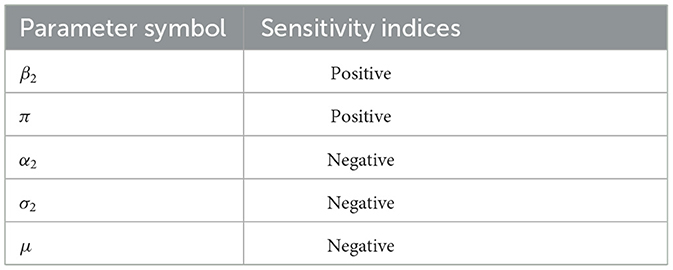
Table 1. Sensitivity indices table.

The results demonstrated that, while the other parameters stayed constant, the parameters with a positive sensitivity index enhanced the value of the reproduction number as their values grew. Furthermore, the value of the reproduction number falls if the values of the parameters having negative indices are raised while the values of the other parameters stay the same. Those parameters that have positive indices (β₂) have a high impact on expanding the disease in the community if their values are increasing. The basic parameters with negative sensitivity indices (α₂, σ₂) increase the disease if their values decrease while the other parameters remain constant. However, increasing human mortality rates to combat disease epidemics is unethical, so they are not taken into account in the study of sensitivity analysis.

3.2 Pneumonia sub-model

The Pneumonia only sub-model is obtained by excluding the COVID-19 infection from the coinfection model,

$\begin{array}{ll}\{\begin{array}{l}\frac{dS}{dt}=\pi +\eta R-({\beta }_1{I}_p+\mu )S,\\ \frac{d{I}_p}{dt}={\beta }_1{I}_{p}S-({\alpha }_1+{\sigma }_1+\mu )I_p,\\ \frac{dR}{dt}={\sigma }_1{I}_p-(\eta +\mu )R.\end{array}& (3)\end{array}$

3.2.1 Disease-free and reproduction number

The disease-free equilibrium (DFE) of the pneumonia sub-model is denoted by ${\Xi }_0^p$ and obtained by setting the right-hand side of system 3 to zero and putting I_p = 0, which is given by

$\begin{array}{l}{\Xi }_0^p=\left(\frac{\pi }{\mu },0,0\right).\end{array}$

Using the next-generation matrix approach, the basic reproduction number of pneumonia sub-model is denoted by ${\mathcal{R}}_0^p$ is

$\begin{array}{l}{\mathcal{R}}_0^p=\frac{\pi {\beta }_1}{\mu ({\alpha }_1+{\sigma }_1+\mu )}.\end{array}$

3.2.2 Stability of disease-free equilibrium

Theorem 3.4. The DFE is locally asymptotically stable if ${\mathcal{R}}_0^p<1$ and unstable if ${\mathcal{R}}_0^p>1$.

Proof. The Jacobian matrix of system 3 at the ${\Xi }_0^p$ is

$\begin{array}{l}{J}_{{\Xi }_0^p}=\left(\begin{array}{ccc}-\mu & -\frac{\pi {\beta }_1}{\mu }& \eta \\ 0& \frac{\pi {\beta }_1}{\mu }-({\alpha }_1+{\sigma }_1+\mu )& 0\\ 0& {\sigma }_1& -(\eta +\mu )\end{array}\right).\end{array}$

Here, the eigenvalues for $J_{{\Xi }_0^p}$ are

$\begin{array}{l}{\lambda }_1=-\pi <0,\\ {\lambda }_2=-(\eta +\mu )<0,\\ {\lambda }_3=({\alpha }_1+{\sigma }_1+\mu )({\mathcal{R}}_0^p-1).\end{array}$

Therefore, the DFE is locally asymptomatically stable if ${\mathcal{R}}_0^p<1$ and otherwise unstable.     □

Theorem 3.5. The disease-free equilibrium of the system 3 is globally asymptotically stable if ${\mathcal{R}}_0^p<1$ and unstable if ${\mathcal{R}}_0^p>1$.

Proof. To prove the global stability of the equilibrium point we construct the Lyapunov function as

$\begin{array}{l}L=M{I}_p,\end{array}$

and differentiating with respect to t gives

$\begin{array}{l}\frac{dL}{dt}=M\frac{d{I}_p}{dt}.\end{array}$

Substituting $\frac{d{I}_p}{dt}$ from the system 3, we obtain

$\begin{array}{l}\frac{dL}{dt}=M\left({\beta }_2{I}_{p}S-({\alpha }_1+{\sigma }_1+\mu )\right)I_p,\\ \le M\left(\frac{{\beta }_1\pi }{\mu }-({\alpha }_1+{\sigma }_1+\mu )\right)I_p,\\ =M({\alpha }_1+{\sigma }_1+\mu )\left(\frac{{\beta }_1\pi }{\mu ({\alpha }_1+{\sigma }_1+\mu )}-1\right)I_p.\end{array}$

Take $M=\frac{1}{{\alpha }_1+{\sigma }_1+\mu }$, then we get

$\begin{array}{l}\frac{dL}{dt}=\left(\frac{{\beta }_1\pi }{\mu ({\alpha }_1+{\sigma }_1+\mu )}-1\right)I_p,\\ =\left({\mathcal{R}}_0^p-1\right)I_p.\end{array}$

for $S\le S_0\le \frac{{\beta }_1\pi }{\mu }$ and $\frac{dL}{dt}\le 0$ for ${\mathcal{R}}_0^p\le 1$ and trajectory of the system 3 on which $\frac{dL}{dt}=0$ if and only if I_p = 0. This implies that the only $\frac{dL}{dt}\le 0$ is ${\Xi }_0^p$. Therefore ${\Xi }_0^p$ is globally asymptotically stable in Ω by Lasalle's invariance principle.     □

3.2.3 Stability of endemic equilibrium

The endemic equilibrium point of sub-model 3 is denoted by $E_e^p=(S^{*},I_p^{*},R^{*})$ and it occurs when the disease persist in the community. To obtain it we equate all the model equations 3 to zero. Then we obtain

$\begin{array}{l}{S}^{*}=\frac{{\alpha }_1+{\sigma }_1+\mu }{{\beta }_1}=\frac{\pi }{\mu }\frac{1}{{\mathcal{R}}_0^p},\\ I_p^{*}=\frac{\mu ({\alpha }_1+{\sigma }_1+\mu )-{\beta }_1\pi (\eta +\mu )}{{\beta }_1(\eta {\sigma }_1-(\eta +\mu )({\alpha }_1+{\sigma }_1+\mu ))}=\frac{(\eta +\mu )({\mathcal{R}}_0^p-1)}{\kappa },\\ R^{*}=\frac{{\sigma }_1\left[\mu ({\alpha }_1+{\sigma }_1+\mu )+{\beta }_1\pi \right]}{{\beta }_2\left[\eta {\sigma }_1-(\eta +\mu )({\alpha }_1+{\sigma }_1+\mu )\right]}=\frac{{\sigma }_1({\mathcal{R}}_0^p-1)}{\kappa },\end{array}$

where,

$\begin{array}{l}\kappa =\frac{{\beta }_1\pi (\eta +\mu )-{\sigma }_1\eta {\mathcal{R}}_0^p}{\pi \mu }.\end{array}$

Theorem 3.6. The endemic equilibrium point $E_e^p$ of system 3 is locally asymptotically stable in Ω if ${\mathcal{R}}_0^p>1$.

Proof. The Jacobian of the system 3, is

$\begin{array}{l}J=\left(\begin{array}{ccc}-{\beta }_1{I}_p^{*}-\mu & -{\beta }_1{S}^{*}& \eta \\ {\beta }_1{I}_p^{*}& {\beta }_1{S}^{*}-({\alpha }_1+{\sigma }_1+\mu )& 0\\ 0& {\sigma }_1& -(\eta +\mu )\end{array}\right).\end{array}$

At the endemic equilibrium point $E_e^p$, evaluating the Jacobian matrix J and then solving |J − λI| = 0, the characteristic equation is ${\lambda }^3+{\psi }_1{\lambda }^2+{\psi }_2\lambda +{\psi }_3=0$, where

$\begin{array}{l}{\psi }_1=\frac{\mu ({\alpha }_1+{\sigma }_1+\mu )-{\beta }_2\pi (\eta +\mu )}{\eta {\sigma }_1-({\alpha }_1+{\sigma }_1+\mu )(\eta +\mu )}-(\eta +\mu ),\\ {\psi }_2=\frac{\mu ({\alpha }_1+{\sigma }_1+\mu )-{\beta }_2\pi (\eta +\mu )}{\eta {\sigma }_1-({\alpha }_1+{\sigma }_1+\mu )(\eta +\mu )}(\eta +\mu )+\mu (\eta +\mu ),\\ {\psi }_3=({\alpha }_1+{\sigma }_1+\mu )(\eta +\mu )\mu -\\ \frac{\mu ({\alpha }_1+{\sigma }_1+\mu )-{\beta }_2\pi (\eta +\mu )}{\eta {\sigma }_1-({\alpha }_1+{\sigma }_1+\mu )(\eta +\mu )}\\ \left[(\eta +\mu )({\alpha }_1+{\sigma }_1+\mu )-\eta {\sigma }_1\right].\end{array}$

Using Routh-Hurwitz criterion all roots of characteristic polynomial have negative real parts if and only if ψ₁ > 0, ψ₂ > 0, ψ₃ > 0 and ψ₂ψ₂ > ψ₃ for ${\mathcal{R}}_0^p>1$. Hence, the endemic equilibrium $E_e^p$ is locally asymptotically stable.     □

3.2.4 Sensitivity analysis

The sensitivity analysis for the basic reproduction number of the sub-model parameters given in Eq. 3 using normalized forward sensitivity index of its ${\mathcal{R}}_0^p$ is given by:

$\begin{array}{l}{\Lambda }_{{\beta }_1}^{{\mathcal{R}}_0^p}=\frac{\partial {\mathcal{R}}_0^p}{\partial {\beta }_1}\times \frac{{\beta }_1}{{\mathcal{R}}_0^p}=1,\\ {\Lambda }_{\pi }^{{\mathcal{R}}_0^p}=\frac{\partial {\mathcal{R}}_0^p}{\partial \pi }\times \frac{\pi }{{\mathcal{R}}_0^p}=1,\\ {\Lambda }_{{\alpha }_1}^{{\mathcal{R}}_0^p}=\frac{\partial {\mathcal{R}}_0^p}{\partial {\alpha }_1}\times \frac{{\alpha }_1}{{\mathcal{R}}_0^p}=-\frac{{\alpha }_1}{{\alpha }_1+{\sigma }_1+\mu }<0\\ {\Lambda }_{{\sigma }_1}^{{\mathcal{R}}_0^p}=\frac{\partial {\mathcal{R}}_0^p}{\partial {\sigma }_1}\times \frac{{\sigma }_1}{{\mathcal{R}}_0^p}=-\frac{{\alpha }_1}{{\alpha }_1+{\sigma }_2+\mu }<0,\\ {\Lambda }_{\mu }^{{\mathcal{R}}_0^p}=\frac{\partial {\mathcal{R}}_0^p}{\partial \mu }\times \frac{\mu }{{\mathcal{R}}_0^p}=-\frac{({\alpha }_2+{\sigma }_2+2\mu )}{{\alpha }_2+{\sigma }_2+\mu }.\end{array}$

The sensitivity indices of the basic reproductive number with respect to main parameters are found in Table 2.

Table 2

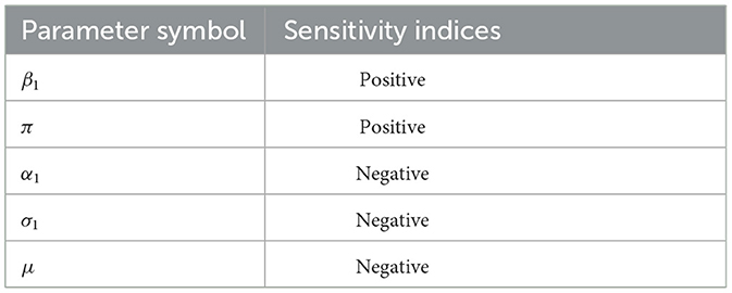
Table 2. Sensitivity indices table.

The sensitivity indices of the basic reproductive number with respect to main parameters are β₁, σ₁, and α₁. When the values of factors with positive sensitivity indices, especially β₁, are raised while the values of the other parameters remain constant, the impact on the spread of the disease is significant. Also those parameters in which their sensitivity indices are negative α₂, σ₂, and μ have an effect of minimizing the burden of the disease in the community as their values increase.

3.3 Co-infection model

In this subsection, will examine the system 1 without controls from a qualitative perspective.

3.3.1 Disease-free equilibrium and reproduction number

The disease-free equilibrium of the co-infected model is obtained by equating all the right-hand sides of Eq. 1 to zero and then setting zero for all state variables involving infected individuals. Then, solving for the non-infected state variables, we obtain

$\begin{array}{l}{\Xi }_0=\left(\frac{\pi }{\mu },0,0,0,0,0,0\right).\end{array}$

To obtain the ${\mathcal{R}}_0$, we used the next-generation matrix method [32]. By the principle of this method, system 1 can be written as

$\begin{array}{l}\begin{array}{l}\frac{d{I}_p}{dt}=f_{p}S+\sigma \rho I_{pc}-({\xi }_1{f}_c+{\alpha }_1+{\sigma }_1+\mu )I_p,\\ \frac{d{I}_c}{dt}=f_{c}S++\sigma \nu I_{pc}-({\xi }_2{f}_p+{\alpha }_2+{\sigma }_2+\mu )I_c,\\ \frac{d{I}_{pc}}{dt}={\xi }_2{f}_p{I}_c+{\xi }_1{f}_c{I}_p-({\alpha }_3+\sigma +\mu )I_{pc}.\end{array}\end{array}$

The transfer matrix are given by

$\begin{array}{l}\mathcal{F}{\mathcal{V}}^{-1}=\left(\begin{array}{ccc}\frac{\pi {\beta }_1}{\mu ({\alpha }_1+{\sigma }_1+\mu )}& 0& \frac{\pi {\beta }_1}{\mu (\sigma +{\alpha }_1+{\alpha }_2+\mu )}\\ 0& \frac{\pi {\beta }_2}{\mu ({\alpha }_2+{\sigma }_2+\mu )}& \frac{\pi {\beta }_2}{\mu (\sigma +{\alpha }_1+{\alpha }_2+\mu )}\\ 0& 0& 0\end{array}\right).\end{array}$

Then the eigenvalues of $\mathcal{F}{\mathcal{V}}^{-1}$ are

$\begin{array}{l}{\lambda }_1=\frac{\pi {\beta }_1}{\mu ({\alpha }_1+{\sigma }_1+\mu )}={\mathcal{R}}_0^p,\\ {\lambda }_2=\frac{\pi {\beta }_2}{\mu ({\alpha }_2+{\sigma }_2+\mu )}={\mathcal{R}}_0^c,\\ {\lambda }_3=0.\end{array}$

Therefore, the basic reproduction number of the co-infection model is

$\begin{array}{l}{\mathcal{R}}_0=max\left\{{\displaystyle {\mathcal{R}}_0^p},{\mathcal{R}}_0^c\right\}.\end{array}$

3.3.2 Local stability of disease-free equilibrium

Theorem 3.7. The DFE is locally asymptotically stable if ${\mathcal{R}}_0<1$ and unstable if ${\mathcal{R}}_0>1$.

The Jacobian matrix of system 1 at the Ξ₀ is

$\begin{array}{l}\mathcal{J}=\left(\begin{array}{ccccccc}\pi & -\frac{\pi {\beta }_1}{\mu }& -\frac{\pi {\beta }_2}{\mu }& -\frac{\pi ({\beta }_1+{\beta }_2)}{\mu }& 0& 0& \eta \\ 0& \frac{\pi {\beta }_1}{\mu }-A& 0& \frac{\pi {\beta }_1}{\mu }& 0& 0& 0\\ 0& 0& \frac{\pi {\beta }_2}{\mu }-B& \frac{\pi {\beta }_2}{\mu }& 0& 0& 0\\ 0& 0& 0& -C& 0& 0& 0\\ 0& {\sigma }_1& 0& \sigma p& -\gamma -\mu & 0& 0\\ 0& 0& {\sigma }_2& \sigma (1-\rho )\nu & 0& -\delta -\mu & 0\\ 0& 0& 0& \sigma (1-\rho )(1-\nu )& \gamma & \delta & -\eta -\mu \end{array}\right),\end{array}$

where A = α₁ + σ₁ + μ, B = α₂ + σ₂ + μ, C = α₁ + α₂ + σ + μ, and then solve |J − λI| = 0, we get

$\begin{array}{l}{\lambda }_1=-\pi <0,\\ {\lambda }_2=({\alpha }_1+{\sigma }_1+\mu )({\mathcal{R}}_0^p-1),\\ {\lambda }_3=({\alpha }_2+{\sigma }_2+\mu )({\mathcal{R}}_0^c-1),\\ {\lambda }_4=-({\alpha }_1+{\alpha }_2+\sigma +\mu )<0,\\ {\lambda }_5=-(\gamma +\mu )<0,\\ {\lambda }_6=-(\delta +\mu )<0,\\ {\lambda }_7=-(\eta +\mu )<0.\end{array}$

Therefore, the DFE is locally asymptomatically stable if ${\mathcal{R}}_0^p<1$ and ${\mathcal{R}}_0^c<1$, otherwise unstable.

3.3.3 Sensitivity analysis

The normalized sensitivity index definition found in subsection 3.1 was applied in this subsection. Since ${\mathcal{R}}_0=max\left\{{\mathcal{R}}_0^p,{\mathcal{R}}_0^c\right\}$, which means that the sensitivity indexes of ${\mathcal{R}}_0^p$ and ${\mathcal{R}}_0^c$ are conducted under each sub-model. Therefore, the most important parameter is the one that is stated in each sub-model.

3.4 Impact of Pneumonia on COVID-19 infection

To describe the impact of pneumonia on COVID-19 and vice versa, we express ${\mathcal{R}}_0^p$ in terms of ${\mathcal{R}}_0^c$. Since,

$\begin{array}{l}{\mathcal{R}}_0^c=\frac{\pi {\beta }_2}{\mu ({\alpha }_2+{\sigma }_2+\mu )},\\ \Rightarrow \mu =\frac{\pi {\beta }_2}{{\mathcal{R}}_0^c({\alpha }_2+{\sigma }_2+\mu )}.\end{array}$

Then, substituting the expression for μ into ${\mathcal{R}}_0^p$ gives

$\begin{array}{l}{\mathcal{R}}_0^p=\frac{{\mathcal{R}}_{0c}{\beta }_1({\alpha }_2+{\sigma }_2+\mu )}{{\beta }_2({\alpha }_1+{\sigma }_1+\mu )}.\end{array}$

To investigate the impact of the two diseases on each other, we did

$\begin{array}{ll}\frac{\partial {\mathcal{R}}_0^c}{\partial {\mathcal{R}}_0^p}=\frac{{\beta }_2({\alpha }_1+{\sigma }_1+\mu )}{{\beta }_1({\alpha }_2+{\sigma }_2+\mu )}>0.& (4)\end{array}$

Equation 4 shows that an increase in pneumonia infection in the community will have a positive influence on the spread of COVID-19 pandemic.

4 Extension into optimal control

In this section, to achieve the best intervention strategies, we reconsider the system 1 and formulate an optimal control problem with four control variables u₁(t), u₂(t), u₃(t), and u₄(t) where,

1. u₁(t) prevention effort of Pneumonia disease,

2. u₂(t) prevention effort of COVID-19 disease,

3. u₃(t) treatment effort of pneumonia infected individuals, and

4. u₄(t) treatment effort of COVID-19 infected individuals.

After incorporating the controls into the coinfection model, we obtain the following optimal control model

$\begin{array}{ll}\{\begin{array}{l}\frac{dS}{dt}=\pi +\eta R-[(1-u_1)f_p+(1-u_2)f_c+\mu ]S,\\ \frac{d{I}_p}{dt}=(1-u_1)f_{p}S+\sigma \rho I_{pc}-((1-u_2)f_c+{\alpha }_1+{\sigma }_1+u_3+\mu )I_p,\\ \frac{d{I}_c}{dt}=(1-u_2)f_{c}S+\sigma \nu I_{pc}-((1-u_1)f_p+{\alpha }_2+{\sigma }_2+u_4+\mu )I_c,\\ \frac{d{I}_{pc}}{dt}=(1-u_2)f_c{I}_p+(1-u_1)f_p{I}_c-({\alpha }_3+\sigma +u_3+u_4+\mu )I_{pc},\\ \frac{dR}{dt}=((1-(\nu +\rho ))\sigma +u_3+u_4)I_{pc}+({\sigma }_2+u_4)I_c+({\sigma }_1+u_3)I_p-\\ (\eta +\mu )R.\end{array}& (5)\end{array}$

To study the optimal levels of the controls, the control set U is Lebesgue measurable and is defined as

$\begin{array}{ll}U=\left\{u_i(t):0\le u_i<1,i=1,\dots ,4,0\le t\le T\right\}.& (6)\end{array}$

The aim of introducing the control variables is to seek the optimal solution required to minimize the numbers of infected individuals responsible for spreading the novel Corona virus and pneumonia in the population at minimum cost. Hence, the objective functional for this control problem is given by

$\begin{array}{ll}\mathcal{J}={\displaystyle \underset{u}{min}}{\displaystyle {\int }_0^T}\left(c_1{I}_p+c_2{I}_c+c_3{I}_{pc}+\frac{1}{2}{\displaystyle \sum _{i=1}^4}{w}_i{u}_i^2\right)dt& (7)\end{array}$

subject to the terms of the model system 5. The parameters w_ifori = 1, 2, 3, 4 measure relative cost of the interventions associated with the controls u_ifori = 1, 2, 3, 4 and the coefficients c₁, c₂, c₃ represents the weight constants corresponding to infected individuals that can be chosen to balance cost factors and is quadratic in the other pieces of literature [34, 35]. Our aim is to minimize the number of infections and costs. Thus, we want to obtain an optimal controls $(u_1^{*},u_2^{*},u_3^{*},u_4^{*})$ in which:

$\begin{array}{ll}\mathcal{J}(u_1^{*},u_2^{*},u_3^{*},u_4^{*})=min\left\{\mathcal{J}(u_1,u_2,u_3,u_4):u_i\in U\right\}.& (8)\end{array}$

4.1 Existence of optimal controls

In this subsection, we prove the existence of such optimal control functions which minimize the cost function in the finite intervention period.

Theorem 4.1. There exists an optimal control pair $(u_1^{*},u_2^{*},u_3^{*},u_4^{*})$ and corresponding solution vector $(S^{*},I_p^{*},I_c^{*},I_{pc}^{*},R^{*})$ to the control induced state initial value problem 5 that minimizes the cost functional J(u₁, u₂, u₃, u₄) over the set of admissible control U 6.

Proof. All the state variable involved in the model are continuously differentiable. Therefore, we need to verify the following four conditions given in Fleming and Rishel [36].

  i. The set of all solutions to Eq. 5 with corresponding control functions in U is nonempty.

 ii. The control set is convex and closed.

iii. The integrand of the objective functional of Eq. 7 is convex.

 iv. The integrand F(t, S, I_p, I_c, I_pc, R, u) in Eq. 7 is convex with respect to control variables and additionally fulfills that F(t, S, I_p, I_c, I_pc, R, u) ≥ g(u), where g is continuous and ‖u‖⁻¹g(u) → +∞ as ‖u‖ → ∞.

In order to established condition (i), we refer to Picard-Lindelöf existence theorem [37]. If the solutions of the state equations are a prior bounded and if the state equations are continuous and Lipschitz continuous in the state variables, then there is a unique solution corresponding to every admissible control in the given domain. With the result that, if g(t, x, u) is bounded, continuous, and Lipschitz in the state variable, then there exists a unique solution corresponding to every admissible control U. Hence, for any u ∈ U and the state variables, we have

$\begin{array}{ll}0\le N(t)\le \frac{\pi }{\mu },& (9)\end{array}$

and nonempty by model assumption. Furthermore, with the bounded established in 5, clearly, the state system is continuous and bounded. It is possible to show the boundedness of the partial derivative with respect to the state variable, i.e., $\frac{\partial g}{\partial x}$, exists and is finite, which establishes that the system is Lipschitz with respect to the state variables [37]. This shows that the proof of condition (i) is complete.

To prove (ii), consider

$\text{U}=\{u\in {ℝ}^4:|\left|u\right||\le 1, ||·|| \text{ is an Euclidean norm}\}.$

Moreover, for any two points y, z ∈ U such that y = (y₁, y₂, y₃, y₄) and z = (z₁, z₂, z₃, z₄). Then for any λ ∈ [0, 1], it follows λy_i + (1 − λ)z_i ∈ U_i, i = 1, 2, 3, 4. This implies that the control set U is convex and closed.

Next we verify condition (iii), the integral of the cost function is given by

$\begin{array}{l}F(t,x,u)=c_1{I}_p+c_2{I}_c+c_3{I}_{pc}+\frac{1}{2}{\displaystyle \sum _{i=1}^4}{w}_i{u}_i^2\end{array}$

where x denotes the state variable and u represents the control variable. To prove condition (iii), we want to prove for any θ ∈ (01) such that,

$\begin{array}{l}(1-\theta )F(t,x,u)+\theta F(t,x,v)\ge F(t,x,(1-\theta )u+\theta v),\end{array}$

where,

$\begin{array}{l}(1-\theta )F(t,x,u)+\theta F(t,x,v)=c_1{I}_p+c_2{I}_c+c_3{I}_{pc}+\\ \frac{1-\theta }{2}{\displaystyle {\sum }_{i=1}^4}{w}_i{u}_i^2+\frac{\theta }{2}{\displaystyle {\sum }_{i=1}^4}{w}_i{v}_i^2,\end{array}$

and

$\begin{array}{l}F(t,x,(1-\theta )u+\theta v)=c_1{I}_p+c_2{I}_c+c_3{I}_{pc}+\frac{1}{2}{\displaystyle \sum _{i=1}^4}{w}_i{((1-\theta )u_i+\theta v_i)}^2.\end{array}$

Therefore,

$\begin{array}{l}F(t,x,v)-F(t,x,(1-\theta )u+\theta v)=\\ \frac{1-\theta }{2}{\displaystyle \sum _{i=1}^4}{w}_i{u}_i^2+\frac{\theta }{2}{\displaystyle \sum _{i=1}^4}{w}_i{v}_i^2-\frac{1}{2}{\displaystyle \sum _{i=1}^4}{w}_i{((1-\theta )u_i+\theta v_i)}^2,\\ =\frac{1}{2}{\displaystyle \sum _{i=1}^4}{w}_i\left[(1-\theta )u_i^2+\theta v_i^2-{((1-\theta )u_i+\theta v_i)}^2\right],\\ =\frac{1}{2}{\displaystyle \sum _{i=1}^4}{w}_i{\left(\sqrt{((1-\theta )\theta )}{u}_i-\sqrt{((1-\theta )\theta )}{v}_i\right)}^2,\\ =\frac{\theta (1-\theta )}{2}{\displaystyle \sum _{i=1}^4}{w}_i{(u_i-v_i)}^2\ge 0.\end{array}$

Hence, (1 − θ)F(t, x, u) + θF(t, x, v) ≥ F(t, x, (1 − θ)u + θv). Therefore, F(t, x, u) is convex. This completes the proof.     □

4.2 The Hamiltonian and optimality system

By using the principle Pontryagin's Manimum Principle [38], we got the necessary conditions which is satisfied by optimal pairs. Therefore, by this principle, we obtained a Hamiltonian ($\mathcal{H}$) defined as

$\begin{array}{l}\mathcal{H}=L+N,\end{array}$

where

$\begin{array}{l}N={\lambda }_1\frac{dS}{dt}+{\lambda }_2\frac{d{I}_p}{dt}+{\lambda }_3\frac{d{I}_c}{dt}+{\lambda }_4\frac{d{I}_{pc}}{dt}+{\lambda }_5\frac{dR}{dt},\end{array}$

and

$\begin{array}{l}L=c_1{I}_p+c_2{I}_c+c_3{I}_{pc}+\frac{1}{2}{\displaystyle \sum _{i=1}^4}{w}_i{u}_i^2.\end{array}$

It follows that the system of Eqs 6 and 5 are substituted into a minimize Hamiltonian function with respect to $u_1^{*},u_2^{*},u_3^{*},u_4^{*}$, we obtain

$\begin{array}{l}\mathscr{H}=c_1{I}_p+c_2{I}_c+c_3{I}_{pc}+\frac{1}{2}{\displaystyle \sum _{i=1}^4{w}_i}{u}_i^2\\ +{\lambda }_1\left[\pi +\eta R-((1-u_1)f_p+(1-u_2)f_c+\mu )S\right]\\ +{\lambda }_2\left[(1-u_1)f_{p}S+\sigma \rho I_{pc}-((1-u_2){\xi }_1{f}_c+{\alpha }_1+{\sigma }_1+u_3+\mu )I_p\right]\\ +{\lambda }_3\left[(1-u_2)f_{c}S+\sigma \nu I_{pc}-((1-u_1){\xi }_2{f}_p+{\alpha }_2+{\sigma }_2+u_4+\mu )I_c\right]\\ +{\lambda }_4\left[(1-u_2){\xi }_1{f}_c{I}_p+(1-u_1){\xi }_2{f}_p{I}_c-({\alpha }_3+\sigma +u_3+u_4+\mu )I_{pc}\right]\\ +{\lambda }_5[((1-(\nu +\rho ))\sigma +u_3+u_4)I_{pc}+({\sigma }_2+u_4)I_c+({\sigma }_1+u_3)I_p-\\ (\eta +\mu )R],& (10)\end{array}$

where λ_i, fori = 1, …, 5 are adjoint variables. Next to obtain the adjoint variables by applying Pontryagin's minimum principle, the following theorem is stated.

Theorem 4.2. For an optimal control set $u_1^{*},u_2^{*},u_3^{*},u_4^{*}$ that minimizes J over U, there is an adjoint variables, λ_i, fori = 1, …, 5 such that:

$\begin{array}{l}\frac{d{\lambda }_1}{dt}=({\lambda }_1-{\lambda }_2)(1-u_1){\beta }_1(I_p+I_{pc})+({\lambda }_1-{\lambda }_3){\beta }_2(1-u_2)(I_c+I_{pc}),\\ \frac{d{\lambda }_2}{dt}=({\lambda }_1-{\lambda }_2){\beta }_1(1-u_1)S+({\lambda }_2-{\lambda }_4){\xi }_1{\beta }_2(1-u_2)(I_c+I_{pc})+({\lambda }_3-\\ {\lambda }_4)(1-u_1){\beta }_1{\xi }_2{I}_c+({\lambda }_2-{\lambda }_5)({\sigma }_1+u_3)+{\lambda }_2({\alpha }_1+\mu )-c_1,\\ \frac{d{\lambda }_3}{dt}=({\lambda }_1-{\lambda }_3)(1-u_2){\beta }_{2}S+({\lambda }_2-{\lambda }_4)(1-u_2){\xi }_1{\beta }_2{I}_p+({\lambda }_3-{\lambda }_4)\\ (1-u_1)(I_p+I_{pc}){\xi }_2{\beta }_1+({\lambda }_3-{\lambda }_5)({\sigma }_2+u_4)+{\lambda }_3({\alpha }_2+\mu )-c_2,\\ \frac{d{\lambda }_4}{dt}=({\lambda }_1-{\lambda }_2)(1-u_1){\beta }_{1}S+({\lambda }_1-{\lambda }_3)(1-u_2){\beta }_{2}S+({\lambda }_2-{\lambda }_4)(1-u_2){\xi }_1{\beta }_2{I}_p\\ +({\lambda }_3-{\lambda }_4)(1-u_1){\xi }_2{\beta }_1{I}_c+({\lambda }_4-{\lambda }_5)(\sigma +u_3+u_4)+({\lambda }_5-{\lambda }_2)\sigma \rho +\\ ({\lambda }_5-{\lambda }_3)\sigma \nu -c_3,\\ \frac{d{\lambda }_5}{dt}=({\lambda }_5-{\lambda }_1)\eta +{\lambda }_5\mu ,& (11)\end{array}$

with the terminal (transversality) conditions

$\begin{array}{ll}{\lambda }_i(T)=0,\text{for }i=1,2,\dots ,5.& (12)\end{array}$

Furthermore, the optimal controls $u_1^{*},u_2^{*},u_3^{*},u_4^{*}$ are represented by

$\begin{array}{l}{u}_1^{*}=min\{max\{0,{\phi }_1\},1\},\\ u_2^{*}=min\{max\{0,{\phi }_2\},1\},\\ u_3^{*}=min\{max\{0,{\phi }_3\},1\},\\ u_4^{*}=min\{max\{0,{\phi }_4\},1\},\end{array}$

where

$\begin{array}{l}{\phi }_1=\frac{({\lambda }_2-{\lambda }_1)(I_p+I_{pc}){\beta }_{1}S+({\lambda }_4-{\lambda }_3)(I_p+I_{pc})I_c{\xi }_2{\beta }_1}{w_1},\\ {\phi }_2=\frac{({\lambda }_3-{\lambda }_1)(I_c+I_{pc}){\beta }_{2}S+({\lambda }_4-{\lambda }_2)(I_c+I_{pc}){\xi }_1{\beta }_2{I}_p}{w_2},\\ {\phi }_3=\frac{({\lambda }_2-{\lambda }_5)I_p+({\lambda }_4-{\lambda }_5)I_{pc}}{w_3},\\ {\phi }_4=\frac{({\lambda }_3-{\lambda }_5)I_c+({\lambda }_4-{\lambda }_5)I_{pc}}{w_4}.\end{array}$

Proof. To obtain the form of the adjoint equations we compute the derivative of the Hamiltonian function ($\mathcal{H}$) Eq. 10 with respect to S, I_p, I_c, I_pc, and R respectively. Then, the adjoint or co-state equation obtained are given by

$\begin{array}{l}\frac{d{\lambda }_1}{dt}=-\frac{\partial \mathscr{H}}{\partial S}=({\lambda }_1-{\lambda }_2)(1-u_1){\beta }_1(I_p+I_{pc})+({\lambda }_1-{\lambda }_3){\beta }_2(1-u_2)(I_c+I_{pc}),\\ \frac{d{\lambda }_2}{dt}=-\frac{\partial \mathscr{H}}{\partial I_p}=({\lambda }_1-{\lambda }_2){\beta }_1(1-u_1)S+({\lambda }_2-{\lambda }_4){\xi }_1{\beta }_2(1-u_2)(I_c+I_{pc})+({\lambda }_3-\\ {\lambda }_4)(1-u_1){\beta }_1{\xi }_2{I}_c+({\lambda }_2-{\lambda }_5)({\sigma }_1+u_3)+{\lambda }_2({\alpha }_1+\mu )-c_1,\\ \frac{d{\lambda }_3}{dt}=-\frac{\partial \mathscr{H}}{\partial I_c}=({\lambda }_1-{\lambda }_3)(1-u_2){\beta }_{2}S+({\lambda }_2-{\lambda }_4)(1-u_2){\xi }_1{\beta }_2{I}_p+({\lambda }_3-{\lambda }_4)\\ (1-u_1)(I_p+I_{pc}){\xi }_2{\beta }_1+({\lambda }_3-{\lambda }_5)({\sigma }_2+u_4)+{\lambda }_3({\alpha }_2+\mu )-c_2,\\ \frac{d{\lambda }_4}{dt}=-\frac{\partial \mathscr{H}}{\partial I_{pc}}=({\lambda }_1-{\lambda }_2)(1-u_1){\beta }_{1}S+({\lambda }_1-{\lambda }_3)(1-u_2){\beta }_{2}S+({\lambda }_2-{\lambda }_4)\\ (1-u_2){\xi }_1{\beta }_2{I}_p+({\lambda }_3-{\lambda }_4)(1-u_1){\xi }_2{\beta }_1{I}_c+({\lambda }_4-{\lambda }_5)(\sigma +u_3+u_4)+\\ ({\lambda }_5-{\lambda }_2)\sigma \rho +({\lambda }_5-{\lambda }_3)\sigma \nu -c_3,\\ \frac{d{\lambda }_5}{dt}=-\frac{\partial \mathscr{H}}{\partial R}=({\lambda }_5-{\lambda }_1)\eta +{\lambda }_5\mu ,\end{array}$

with transversality conditions.

To obtain the controls value, we compute the partial derivative of Hamiltonian given by

$\begin{array}{l}\frac{\partial \mathcal{H}}{\partial u_i}=0,\text{for }i=1,2,\dots ,4.\end{array}$

Obviously, after derivation of Hamiltonian ($\mathcal{H}$) with respect to the controls the result becomes

$\begin{array}{ll}\{\begin{array}{l}\frac{\partial \mathcal{H}}{\partial u_1}=0=w_1{u}_1+({\lambda }_1-{\lambda }_2)(I_p+I_{pc}){\beta }_{1}S+({\lambda }_3-{\lambda }_4)(I_p+I_{pc})I_c{\beta }_1{\xi }_2,\\ \frac{\partial \mathcal{H}}{\partial u_2}=0=w_2{u}_2+({\lambda }_1-{\lambda }_3){\beta }_2(I_c+I_{pc})S+({\lambda }_2-{\lambda }_4){\xi }_1{\beta }_2(I_c+I_{pc}),\\ \frac{\partial \mathcal{H}}{\partial u_3}=0=w_3{u}_3+({\lambda }_5-{\lambda }_2)I_p+({\lambda }_5-{\lambda }_4)I_{pc},\\ \frac{\partial \mathcal{H}}{\partial u_4}=0=w_4{u}_4+({\lambda }_5-{\lambda }_3)I_c+({\lambda }_5-{\lambda }_4)I_{pc}.\end{array}& (13)\end{array}$

Then, solve for (u₁, u₂, u₃, u₄), we obtain

$\begin{array}{l}\{\begin{array}{l}{u}_1^{*}=\frac{({\lambda }_2-{\lambda }_1)(I_p+I_{pc}){\beta }_{1}S+({\lambda }_4-{\lambda }_3)(I_p+I_{pc})I_c{\xi }_2{\beta }_1}{w_1},\\ u_2^{*}=\frac{({\lambda }_3-{\lambda }_1)(I_c+I_{pc}){\beta }_{2}S+({\lambda }_4-{\lambda }_2)(I_c+I_{pc}){\xi }_1{\beta }_2{I}_p}{w_2},\\ u_3^{*}=\frac{({\lambda }_2-{\lambda }_5)I_p+({\lambda }_4-{\lambda }_5)I_{pc}}{w_3},\\ u_4^{*}=\frac{({\lambda }_3-{\lambda }_5)I_c+({\lambda }_4-{\lambda }_5)I_{pc}}{w_4}.\end{array}\end{array}$

From boundedness on $u_i^{*}$(t) and minimality condition, we have:

$\begin{array}{l}{u}_1^{*}=min\{max\{0,{\phi }_1\},1\},\\ u_2^{*}=min\{max\{0,{\phi }_2\},1\},\\ u_3^{*}=min\{max\{0,{\phi }_3\},1\},\\ u_4^{*}=min\{max\{0,{\phi }_4\},1\},\end{array}$

where

$\begin{array}{l}{\phi }_1=\frac{({\lambda }_2-{\lambda }_1)(I_p+I_{pc}){\beta }_{1}S+({\lambda }_4-{\lambda }_3)(I_p+I_{pc})I_c{\xi }_2{\beta }_1}{w_1},\\ {\phi }_2=\frac{({\lambda }_3-{\lambda }_1)(I_c+I_{pc}){\beta }_{2}S+({\lambda }_4-{\lambda }_2)(I_c+I_{pc}){\xi }_1{\beta }_2{I}_p}{w_2},\\ {\phi }_3=\frac{({\lambda }_2-{\lambda }_5)I_p+({\lambda }_4-{\lambda }_5)I_{pc}}{w_3},\\ {\phi }_4=\frac{({\lambda }_3-{\lambda }_5)I_c+({\lambda }_4-{\lambda }_5)I_{pc}}{w_4}.\end{array}$

This completes the proof of the theorem.     □

5 Numerical simulations

In this section, we illustrate numerically the solution of the optimal control problem proposed in system 1 and Table 3. For this purpose, we use the forward-backward sweep method presented in the book of Lenhart and Workman [39].

Table 3

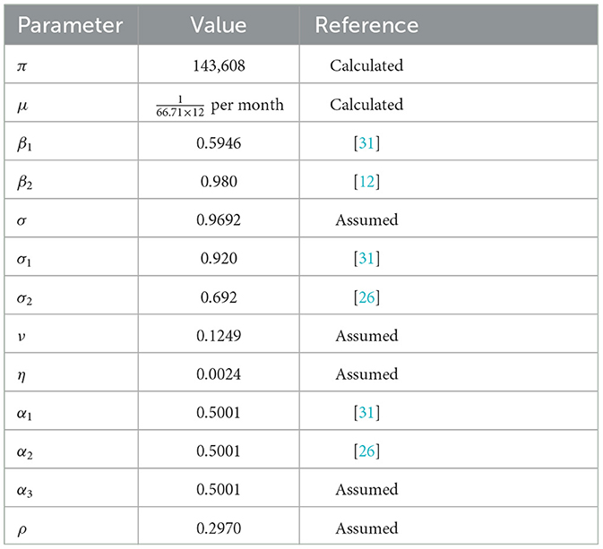
Table 3. The values of parameters used in the simulations.

To briefly summarize the numerical simulation procedure, first we perform forward fourth order Runge-Kutta scheme to solve system 1 over the interval [0, T] with its initial condition and the transversality conditions λ_i(T) = 0; i = 1, 2, 3, 4, 5, where T = 35 is simulation time. Incontrary, we use backward fourth order Runge-Kutta scheme to solve system 10 using the current iteration solution of 1. The control is updated by using a convex combination of the previous control and the values computed in the characterizations process. The iteration continuous until the values of the unknowns at the previous iteration are very close to the values of present iteration. To perform the numerical simulation, we assumed the initial population of

$(S(0),I_p(0),I_c(0),I_{pc}(0),R(0))=(5,000,000,550,26,10,400)$

The natural death rate is computed as $\mu =\frac{1}{66.71\times 12}$ per month, where 66.71 years is the average life expectancy in Ethiopia [40]. The recruitment rate, is then calculated as π = μ × N(0) = 143, 608 per month, where N(0)= 114,961,850.

The cost coefficients corresponding to control variables are estimated to be c₁ = 25, c₂ = 75, and c₃ = 55 the relative importance of reducing the associated classes on the spread of the disease are w₁ = 3, w₂ = 8, w₃ = 7 and w₄ = 5. Using all necessary information above, we analysis and compare the numerical results of the effect of controls on the spread of COVID-19 in populations.

1. Scenario A (using combinations of two controls):

-Strategy 1: Applying both the COVID-19 and pneumonia prevention method (u₁ ≠ 0, u₂ ≠ 0, u₃ = 0, u₄ = 0).

-Strategy 2: Applying Pneumonia prevention method and treatment for pneumonia (u₁ ≠ 0, u₂ = 0, u₃ ≠ 0, u₄ = 0).

-Strategy 3: Applying Pneumonia prevention method and treatment for COVID-19 (u₁ ≠ 0, u₂ = 0, u₃ = 0, u₄ ≠ 0).

-Strategy 4: Applying COVID-19 prevention method and treatment for pneumonia (u₁ = 0, u₂ ≠ 0, u₃ ≠ 0, u₄ = 0).

-Strategy 5: Applying COVID-19 prevention method and treatment for COVID-19 (u₁ = 0, u₂ ≠ 0, u₃ = 0, u₄ ≠ 0).

-Strategy 6: Applying both the Pneumonia and COVID-19 treatment method (u₁ = 0, u₂ = 0, u₃ ≠ 0, u₄ ≠ 0).

2. Scenario B (using triple controls)

-Strategy 7: Applying both the Pneumonia and COVID-19 prevention method and treatment for Pneumonia (u₁ ≠ 0, u₂ ≠ 0, u₃ ≠ 0, u₄ = 0).

-Strategy 8: Applying both the Pneumonia and COVID-19 prevention and treatment for COVID-19 (u₁ ≠ 0, u₂ ≠ 0, u₃ = 0, u₄ ≠ 0).

-Strategy 9: Applying Pneumonia prevention method and, treatment for Pneumonia and COVID-19 (u₁ ≠ 0, u₂ = 0, u₃ ≠ 0, u₄ ≠ 0).

-Strategy 10: Applying COVID-19 prevention method, and treatment for both Pneumonia and COVID-19 (u₁ = 0, u₂ ≠ 0, u₃ ≠ 0, u₄ ≠ 0).

3. Scenario C (using all controls)

Using all controls means u₁ ≠ 0, u₂ ≠ 0, u₃ ≠ 0, u₄ ≠ 0.

5.1 Scenario A

Under Scenario A, we consider combinations of two controls. Numerical simulations are showed in Figures 2A–C. Figure 2A shows that controls with prevention and treatment of Pneumonia disease (Strategy 2) have a potential of decreasing the number of pneumonia infected populations. However, a control with treatment effort only for both disease (Strategy 3) takes more time to decrease the number of pneumonia infected populations. From the Figure 2B shows that controls with treatment effort only for both disease (Strategy 6) decreases the number of co-infectious, Pneumonia infectious and COVID-19 infectious population goes down in the specified time. Figure 2C shows that the Strategy 2 and Strategy 6 have more potential to decreasing number of infected individuals under the scenario A. Ingeneral, we conclude that applying an optimized controls can eradicate both diseases from the community in a specified period of time.

Figure 2

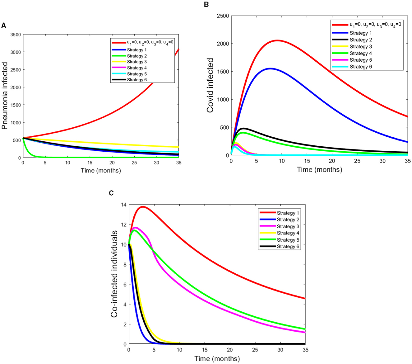
Figure 2. (A–C) Simulations of pneumonia infected, COVID-19 infected and pneumonia with COVID-19 coinfection with applying the strategies under Scenario A.

5.2 Scenario B

Under this scenario, we considered the combinations of three controls. The simulation results from Figure 3A shows that a control with prevention of Pneumonia disease and treatment of both COVID-19 and Pneumonia disease have a potential of decreasing the co-infectious, Pneumonia infectious and COVID-19 infectious populations. From these four strategies, Strategy 9 rapidly reduces the number of co-infectious, Pneumonia infectious and COVID-19 infectious populations. Figure 3B displays as strategy 10 has a great role in decreasing the burden of COVID-19 disease. Also from Figure 3C we can see that as strategy 7 and 9 have a good approach in reducing the number of coinfected populations.

Figure 3

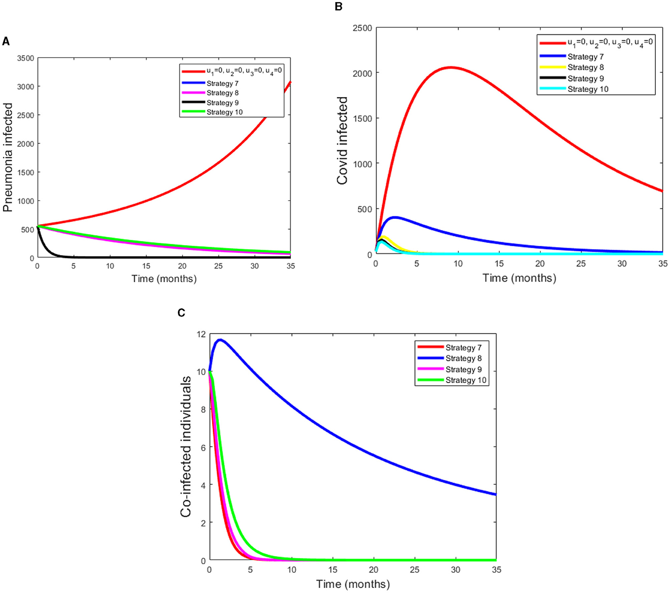
Figure 3. (A–C) Simulations of pneumonia infected, COVID-19 infected and coinfection with applying Scenario B.

5.3 Scenario C

Under this scenario, we determined the difference between the compartment with control and without control. We considered four controls at the same time. Figure 4A shows that pneumonia infected compartment is rapidly decreased when we apply all controls. Also Figure 4B displays COVID-19 can be eradicated in a short time if we apply all controls. From the Figure 4C, we can see that as coinfected populations with controls are drammatically decreased.

Figure 4

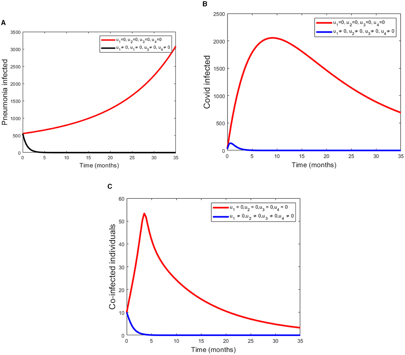
Figure 4. (A–C) Simulations of Pneumonia infected, COVID-19 infected and the coinfection of Pneumonia and COVID-19 using all four controls.

6 Conclusions

In this paper, we proposed and analyzed a deterministic mathematical model for the co-infection of COVID-19 with pneumonia. The co-infection model is divided into two submodels, namely, the pneumonia-only submodel and the COVID-19-only submodel. The well-posedness of the model was established both in the mathematical and epidemiological sense by showing that all solutions to the model are positive and bound with initial conditions in a certain meaningful set. The equilibrium and basic reproduction numbers are computed for the co-infection model and each submodel independently. The basic reproduction number of the co-infection model is shown to be the greatest of the reproduction numbers of the two sub-models. It is observed that both submodels and the full co-infection models have locally asymptotically stable disease-free equilibrium when their respective basic reproduction numbers are less than unity and otherwise unstable. Furthermore, there exists a stable endemic equilibrium point for the basic reproduction numbers greater than one. A sensitivity analysis of the model was performed and identified the positive and negative index parameters. From the basic model, an optimal control problem is formulated by incorporating two control variables: prevention, treatment, and their combination. The Hamiltonian, adjoint variables, the characterization of the controls and the optimality system are derived from the optimal control problem and also numerically simulated by considering a single control at a time, a combination of two controls at a time, and lastly, by applying all three control variables. Several combinations of the control variables are compared to determine which combination is most effective in the fight against pneumonia and COVID-19.

Data availability statement

The original contributions presented in the study are included in the article/supplementary material, further inquiries can be directed to the corresponding author.

Author contributions

BA: Conceptualization, Data curation, Formal analysis, Investigation, Resources, Validation, Writing—original draft. TK: Supervision, Writing—review & editing. DT: Formal analysis, Software, Validation, Writing—review & editing. HB: Validation, Supervision, Review, Editing.

Funding

The author(s) declare that no financial support was received for the research, authorship, and/or publication of this article.

Conflict of interest

The authors declare that the research was conducted in the absence of any commercial or financial relationships that could be construed as a potential conflict of interest.

Publisher's note

All claims expressed in this article are solely those of the authors and do not necessarily represent those of their affiliated organizations, or those of the publisher, the editors and the reviewers. Any product that may be evaluated in this article, or claim that may be made by its manufacturer, is not guaranteed or endorsed by the publisher.

References

1. World Health Organization (WHO). Pneumonia Fact Sheet: Media Centre. Geneva: WHO (2013).

Google Scholar

2. United Nations Childrens Fund (UNICEF). Childhood Pneumonia: Everything you need to Know. (2020). Available online at: https://www.unicef.org/stories/childhood-pneumonia-explained/ (accessed August 20, 2021).

Google Scholar

3. World Health Organization (WHO). Technical Basis for the WHO Recommendations on the Management of Pneumonia in Children at First Level Health Facilities. Geneva: WHO (2008).

Google Scholar

4. World Health Organization (WHO). Coronavirus Disease 2019 (COVID-19): Situation Report, 68. Geneva: WHO (2020).

Google Scholar

5. World Health Organization. COVID-19 Weekly Epidemiological Update, Edition 70. Geneva: WHO (2021).

Google Scholar

6. Word Heath Organization (WHO). WHO Coronavirus Dashboard. Available online at: https://covid19.who.int

Google Scholar

7. Diekmann O, Heesterbeek J. Mathematical Epidemiology of Infectious Diseases. Hoboken, NJ: Wiley (2000).

Google Scholar

8. Bandekar SR, Ghosh M. Mathematical modeling of COVID-19 in India and its states with optimal control. Model Earth Syst Environ. (2021). doi: 10.1140/epjp/s13360-021-02046-y

PubMed Abstract | Crossref Full Text | Google Scholar

9. Bandekar SR, Ghosh M. Modeling and analysis of COVID-19 in India with treatment function through different phases of lockdown and unlock. Stoch Anal Appl. (2021) 40:812–29. doi: 10.1080/07362994.2021.1962343

Crossref Full Text | Google Scholar

10. Lemecha Obsu L, Feyissa Balcha S. Optimal control strategies for the transmission risk of COVID-19. J Biol Dyn. (2020) 14:590–607. doi: 10.1080/17513758.2020.1788182

PubMed Abstract | Crossref Full Text | Google Scholar

11. Roosa K, Lee Y, Luo R, Kirpich A, Rothenberg R, Hyman JM, et al. Real-time forecasts of the COVID-19 epidemic in china from February 5th to February 24th, 2020. Infect Dis Model. (2020) 5:256–63. doi: 10.1016/j.idm.2020.02.002

PubMed Abstract | Crossref Full Text | Google Scholar

12. Kucharski AJ, Russell TW, Diamond C, Liu Y, Edmunds J, Funk S, et al. Early dynamics of transmission and control of COVID-19: a mathematical modelling study. Lancet Infect Dis. (2020). doi: 10.1101/2020.01.31.20019901

PubMed Abstract | Crossref Full Text | Google Scholar

13. Mekonen KG, Habtemicheal TG, Balcha SF. Modeling the effect of contaminated objects for the transmission dynamics of COVID-19 pandemic with self protection behavior changes. Results Appl Math. (2021) 9:100134. doi: 10.1016/j.rinam.2020.100134

Crossref Full Text | Google Scholar

14. Mamo DK. Model the transmission dynamics of COVID-19 propagation with public health intervention. Results Appl Math. (2020) 7:100123. doi: 10.1016/j.rinam.2020.100123

Crossref Full Text | Google Scholar

15. Smith T, Lehmann D, Montgomery J, Gratten M, Rileyii ID, Alpers MP, et al. Acquisition and invasiveness of different serotypes of streptococcus pneumoniae in young children. Epidemiol Infect. (1993) 111:27–39. doi: 10.1017/S0950268800056648

PubMed Abstract | Crossref Full Text | Google Scholar

16. Lipsitch M. Bacterial vaccines and serotype replacement: lessons from haemophilus influenzae and prospects for streptococcus pneumoniae. Emerg Infect Dis. (1999) 5:336–45. doi: 10.3201/eid0503.990304

PubMed Abstract | Crossref Full Text | Google Scholar

17. Temime L, Guillemot D, Boelle PYB. Short and long term effects of pneumococcal conjugate vaccination of children on penicillin resistance. Antimicrob Agents Chemother. (2004) 48:2206–13. doi: 10.1128/AAC.48.6.2206-2213.2004

PubMed Abstract | Crossref Full Text | Google Scholar

18. Melegaro A, Gay NJ, Medley GF. Estimating the transmission parameter of pneumococcal carriage in households. Epidemiol Infect. (2004) 132:133–441. doi: 10.1017/S0950268804001980

PubMed Abstract | Crossref Full Text | Google Scholar

19. Lawi GO, Mugisha JYT, Omolo-Ongati N. Modeling co-infection of paediatric malaria and pneumonia. Int J Math Anal. (2013) 7:413–24. doi: 10.12988/ijma.2013.13037

Crossref Full Text | Google Scholar

20. Farr BM, Bartlett CLR, Wadsworth J, Miller DL. Risk factors for community-acquire pneumonia diagnosed upon hospital admission. Respir Med. (2000) 94:954–63. doi: 10.1053/rmed.2000.0865

Crossref Full Text | Google Scholar

21. Pessoa D. Modelling the Dynamics of Streptococcus pneumoniae Transmission in Children [Masters thesis]. University of Dehisboa (2010).

Google Scholar

22. Singh V, Aneja S. Pneumonia management in the developing world. Paediatr Respir Rev. (2011) 12:52–9. doi: 10.1016/j.prrv.2010.09.011

Crossref Full Text | Google Scholar

23. Tchoumi S, Diagne ML, Rwezaura H, Tchuenche JM. Malaria and COVID-19 co-dynamics: a mathematical model and optimal control. Appl Math Model. (2021) 99:294–327. doi: 10.1016/j.apm.2021.06.016

PubMed Abstract | Crossref Full Text | Google Scholar

24. Rehman AU, Singh R, Agarwal P. Modeling, analysis and prediction of new variants of COVID-19 and dengue co-infection on complex network. Chaos Solitons Fractals. (2021) 150:111008. doi: 10.1016/j.chaos.2021.111008

PubMed Abstract | Crossref Full Text | Google Scholar

25. Omame A, Abbas M. Modeling SARS-CoV-2 and HBV co-dynamics with optimal control. Physica A. (2023). 615:128607. doi: 10.1016/j.physa.2023.128607

PubMed Abstract | Crossref Full Text | Google Scholar

26. Mekonen KG, Balcha SF, Obsu LL, Hassen A. Mathematical modeling and analysis of TB and COVID-19 coinfection. J Appl Math. (2022) 2022:2449710. doi: 10.1155/2022/2449710

Crossref Full Text | Google Scholar

27. Marimuthu Y, Nagappa B, Sharma N, Basu S, Chopra K. COVID-19 and tuberculosis: a mathematical model based forecasting in Delhi, India. Indian J Tuberc. (2020) 67:177–81. doi: 10.1016/j.ijtb.2020.05.006

PubMed Abstract | Crossref Full Text | Google Scholar

28. Omame A, Abbas M, Onyenegecha CP. A fractional-order model for COVID-19 and tuberculosis co-infection using Atangana-Baleanu derivative. Chaos Solitons Fractals. (2021) 153:111486. doi: 10.1016/j.chaos.2021.111486

PubMed Abstract | Crossref Full Text | Google Scholar

29. Adeboye KR, Haruna M. A mathematical model for the transmissionand control of malaria and typhoid co-infection using sirs approach. Niger Res J Math. (2015) 2:1–24.

Google Scholar

30. Akinyi OC, Mugisha JY, Manyonge A, Ouma C. A model on the impact of treating typhoid with anti-malarial: dynamics ofmalaria concurrent and co-infection with typhoid. Appl Math Sci. (2015) 9:541–51. doi: 10.12988/ijma.2015.412403

Crossref Full Text | Google Scholar

31. Tilahun GT, Makinde OD, Malonza D. Co-dynamics of pneumonia and typhoid fever diseases with cost effective optimal control analysis. Appl Math Comput. (2018) 316:438–59. doi: 10.1016/j.amc.2017.07.063

Crossref Full Text | Google Scholar

32. Van den Driessche P, Watmough J. Reproduction numbers and subthreshold endemic equilibria for compartmental models of disease transmission. Math Biosci. (2002) 180:29–48. doi: 10.1016/s0025-5564(02)00108-6

PubMed Abstract | Crossref Full Text | Google Scholar

33. Chitnis N, Hyman JM, Cushing JM. Determining important parameters in the spread of malaria through the sensitivity analysis of a mathematical model. Bull Math Biol. (2008) 70:1272. doi: 10.1007/s11538-008-9299-0

PubMed Abstract | Crossref Full Text | Google Scholar

34. Temesgen DK, Makinde OD, Obsu LL. Optimal control and cost-effectiveness analysis of SIRS malaria disease model with temperature variability factor. J Math Fund Sci. (2021) 53:134–63. doi: 10.5614/j.math.fund.sci.2021.53.1.10

Crossref Full Text | Google Scholar

35. Duressa T, Makinde OD, Obsu L. Impact of temperature variability on SIRS Malaria Model. J Biol Syst. (2021) 29:773–98. doi: 10.1142/S0218339021500170

Crossref Full Text | Google Scholar

36. Fleming WH, Rishel RW. Deterministic and Stochastic Optimal Control, Vol. 1. Berlin: Springer Science & Business Media (2012).

Google Scholar

37. Levinson N, Coddington E. Theory of Ordinary Differential Equations. New York, NY: Tata McGraw-Hill Education (1955).

Google Scholar

38. Pontryagin LS, Boltyanskii VG, Gamkrelize RV, Mishchenko EF. The Mathematical Theory of Optimal Processes. New York, NY: John Wiley & Sons (1986).

Google Scholar

39. Lenhart S, Workman JT. Optimal Control Applied to Biological Models. Boca Raton, FL: CRC press (2007).

Google Scholar

40. WHO (2020). Available online at: https://www.macrotrends.net/countries/eth/ethiopia/life-expectancy

Google Scholar