 Zhitao Wang1†
 Yuanquan Wang
- 1School of Artificial Intelligence, Hebei University of Technology, Tianjin, China
- 2School of Information and Communication Engineering, North University of China, Taiyuan, China
- 3Shanxi Provincial Key Laboratory for Biomedical Imaging and Big Data, North University of China, Taiyuan, China
- 4The Third Central Hospital of Tianjin, Tianjin, China
The active contour model, also known as the snake model, is an elegant approach for image segmentation and motion tracking. The gradient vector flow (GVF) is an effective external force for active contours. However, the GVF model is based on isotropic diffusion and does not take the image structure into account. The GVF snake cannot converge to very deep concavities and blob-like concavities and fails to preserve weak edges neighboring strong ones. To address these limitations, we first propose the directionally weakened diffusion (DWD), which is anisotropic by incorporating the image structure in a subtle way. Using the DWD, a novel external force called directionally weakened gradient vector flow (DWGVF) is proposed for active contours. In addition, two spatiotemporally varying weights are employed to make the DWGVF robust to noise. The DWGVF snake has been assessed on both synthetic and real images. Experimental results show that the DWGVF snake provides much better results in terms of noise robustness, weak edge preserving, and convergence of various concavities when compared with the well-known GVF, the generalized GVF (GGVF) snake.
1 Introduction
SNAKES or active contours, proposed originally by Kass et al. (1) in 1988, are elastic curves that move and change their shapes within an image domain under the control of internal and external forces. The internal force controls the continuity and smoothness of the curve, while the external force, derived from image data, drives the snake contour to approach objects. The snake models provide a good solution for shape modeling of objects in visual data and have gained widespread popularity in the community of computer vision. The active contours can usually be categorized into region-based models (2–22) and edge-based models (1, 23–32) according to how the image data are utilized. The region-based models usually employ certain region homogeneity criteria to guide the evolution of the active contours, such as the local region descriptors in Ref. (12–15) and the histogram in (17). The advantages of region-based models include robustness to noise and weak edge and insensitivity to initial contour. Edge-based models utilize the image edge map to stop the evolution of the contour; as a result, the active contours follow a high gradient to extract object boundaries and are effective only when the contrast between foreground and background is high. Depending on the representation scheme used, active contours can also be classified as a geometric model, which utilizes an implicit representation (33), and a parametric model, which adopts an explicit parametric manner. The region-based active contours always adopt an implicit representation under the level-set framework, and the edge-based models usually take an explicit parametric form. Recently, the deep learning-based approaches have gained popularity in image segmentation (34–37); however, the deep learning methods need a large number of training examples, and the active contours are still an active topic in the computer vision community; for example, the studies in (4, 14, 20–22, 30). In addition, we refer the interested readers to Antonelli et al. (38) for the review of the computational models for image segmentation. In this study, we also focus on the edge-based parametric active contour.
Under the framework of edge-based active contours, the typical external force is derived from the gradient of the edge map. However, this gradient-based external force is ‘myopic’ due to its local nature and not regular enough owing to noise; as a result, the initial snake contour has to be laid close to the object boundary. In order to overcome the shortcomings of this gradient-based external force, Xu and Prince (39, 40) proposed the gradient vector flow (GVF) external force, which largely solved the problem of limited capture range. The graceful behavior of GVF has appealed to many researchers, and there are many improved versions, for example, the motion gradient vector flow (41), the harmonic gradient vector flow (42), the dynamic directional gradient vector flow (43), the boundary vector field (44), the multi-direction gradient vector flow (45), the GVF in normal direction (46), the edge-preserving gradient vector flow (47), the gradient vector convolution (48) and quasi-automatic initialization using gradient vector flow (49), the virtual electric field (50), the normally biased GVF (51), the 4D GVF (52), and the GVF over manifold (53); there are also several interesting applications of GVF (54–59); for instance, Yu and Chua (54) integrated the GVF into anisotropic diffusion for image restoration, Prasad and Yegnanarayana (55) utilized the GVF to find the axes of symmetry, and Hassouna and Farag extracted the object skeleton based on GVF (56).
The GVF is endowed with a large capture range by employing a certain smoothness constraint, which has also been used in optical flow (60). But as pointed out by Nagel (60), ‘this smoothness requirement is applied indiscriminately across all gray value edges despite the fact that such edges might separate image regions’, which signifies that the image structure is not taken into account. This would lead to the fact that the GVF could not preserve weak edges. In this study, we explore the integration of local image structure into the smoothness constraint and thereby present a novel external force, which we call directionally weakened gradient vector flow (DWGVF), for active contours. This DWGVF weakens the diffusion in the gradient direction of the image, and consequently, the DWGVF behaves much better than the GVF and GGVF models.
This study is organized as follows: Section 2 briefly reviews the snake model and four gradient-based external forces; the proposed DWD diffusion and DWGVF snake are presented in Section 3; experiments and comparisons are presented in Section 4, and conclusions are drawn in Section 5.
2 Background
Here, we give a brief review of the active contour model with four well-known gradient-based external forces, which we will later apply for comparison against our proposed external force.
2.1 Snakes: active contours
A snake is a curve c(s) = [x(s),y(s)], that moves and changes its shape by minimizing the following energy function:
where cs(s) and css(s) are the first and second derivatives of c(s) with respect to arc length s and α and β are weighting parameters that control the smoothness and rigidity of the curve, respectively. The external energy Eext(c(s)) is derived from the image data and takes smaller values at the features of interest, such as boundaries. By the calculus of variations, the Euler equation to minimize Esnake is
This can be considered as a force balance equation:
where Fint = αcss(s)- βcssss(s) and Fext= . The internal force Fint keeps the snake contour smooth, while the external force Fext attracts the snake to the desired image features.
The typical external force for gray-value image I is defined as the gradient vector of the edge map, as follows:
where Gσ is the Gaussian kernel with standard deviation σ, denotes convolution, and denotes gradient operator. However, this gradient vector is local and not regular enough to guide the evolution of the snake model. More effective external forces should be developed.
2.2 Gradient vector flow: gradient vector flow external force
In order to overcome the limitations of the typical external force in (4), Xu and Prince proposed to replace Fext in (4) with the GVF external force. The GVF is a vector field obtained by minimizing the following energy functional,
where ux, uy, vx, vy are the spatial derivatives of the field, f is the edge map of an image, μ is a regularization parameter governing the tradeoff between the first term and the second term in Eq. (5). As pointed out in Ref. (39), when is large, the second term in Eq. (5) is dominant and produces the effect of keeping nearly equal to . Whereas when is small, the first term dominates the energy, yielding a slowly varying field. Using the calculus of variations, the Euler equation to minimize reads,
where Δ is the Laplacian operator. As the GVF is derived by diffusing the gradient vector further away from the edges, it greatly enlarges the capture range of the snake and enhances its ability to converge to concavity.
The GGVF is an extension of the GVF by replacing μ and in (6) with two spatially varying functions and , respectively (40); acts as a threshold and controls the smoothing effect. The introduction of such terms makes the GGVF snake behave better than the GVF snake on thin concavity convergence.
2.3 NGVF: gradient vector flow in normal direction
From a viewpoint of image interpolation, Ning et al proposed the gradient vector flow in the normal direction (NGVF) by discarding the second derivative in the tangential direction in the Laplace operator. It is well known that the Laplace operator can be decomposed into two terms, taking as an example,
where and are the second derivatives of in the tangential and normal directions of the isophotes, respectively. It was pointed out in (61–63) that, as an interpolation operator, has the best performance, Δu the second, and the last. By taking the diffusion process in Eq. (6) as an interpolation process, the NGVF is proposed using the best interpolator, as follows:
where is also a positive weight as in Eq. (6).
3 Directionally weakened diffusion and DWGVF snake
3.1 DWD: directionally weakened diffusion
It is clear that the GVF equations in Eq. (6) and the NGVF equations in Eq. (8) are diffusion equations. Diffusion partial differential equations (PDEs) have been one of the most influential tools for image restoration during the last two decades, and it is well-known that the anisotropic PDEs are more competent than its isotropic peers in preserving edges while removing noise. The GVF model is based on isotropic diffusion and the NGVF is based on anisotropic diffusion. However, neither the GVF model nor the NGVF model takes into account the structure of the original image; as a result, the active contour cannot discern objects of complex shapes, such as various concavities and weak edges neighboring strong ones. In order to address this issue, we propose the directionally weakened diffusion (DWD), which incorporates the structure of the original image in a subtle way. Let I(x,y) denote the image, Ix(x,y), Iy(x,y) denote the partial derivatives of I(x,y) with respect to x, y, respectively, is a unitary normal vector of I(x,y), i.e., , is a unitary vector orthogonal to and . Taking u(x,y) as an example, let ux(x,y), uy(x,y) denote the partial derivatives of u(x,y) with respect to x,y, respectively; the second directional derivative of along the normal direction of image I(x,y), i.e., reads
It is different from the in Eqs (7–8) that is the second directional derivative of along the normal direction of itself. Similarly, the second directional derivative of along is as follows:
As a result, the proposed DWD for u(x,y) is as follows,
That is, the diffusion in the direction is weakened, this is the reason why it is called directionally weakened diffusion (DWD in short), and this diffusion possesses three traits,
1. The image structure of image I(x,y), i.e., is incorporated into the diffusion process; it means the diffusion process can refer to any other structure, for example, of image I(x,y), not of u(x,y) itself, in this way.
2. Theoretically, , it means the diffusion extends u(x,y) along the tangential direction of image I(x,y), i.e., the edge direction; in an anisotropic manner, it is helpful to preserve the edge.
3. Meanwhile, when (Ix, Iy) is zero, degenerates to Δu that is isotropic, but if is directly employed, the diffusion stops since when (Ix, Iy) is zero. As a result, the proposed formulation is helpful to diffuse u(x,y) when (Ix, Iy) is zero and preserve edges when (Ix, Iy) is not zero.
These properties make the DWD very suitable to compute the gradient vector flow (GVF) as the GVF aims at recovering the vector field from another one ; the details are presented in the next subsection.
3.2 Directionally weakened gradient vector flow: DWD for gradient vector flow
Based on the novel DWD in the preceding subsection, we argue that the diffusion along the normal direction of should be removed so that the diffusion is anisotropic and tends to preserve the edges of image , not that of . Thus, the proposed GVF based on DWD is derived by solving the following anisotropic diffusion equations,
where and are two spatiotemporally varying weighting functions. This DWGVF model becomes distinctive in two ways:
• Conceptually, equals , which implies that, on high gradient regions ( , hence, ), the current point may be located on an edge; the diffusion along the normal direction of image would be removed, and only that along the tangent direction of image is preserved. This would be beneficial for removing noise and maintaining edges. However, when the local geometry is flat and does not contain any edges ( , hence, ); the diffusion should be isotropic, i.e., with no preferred diffusion direction.
• The two weighting functions and distinguish themselves from the two weights in GGVF as and are spatiotemporally varying while are merely spatially varying. This property makes DWGVF more robust to noise than GGVF because the noise is gradually smoothed away, and and are more and more regular during iteration; therefore, increases and decreases gradually at noise points; hence, a smoother result can be obtained.
These properties signify that the DWGVF is not just a slight modification of the GGVF. In order to illustrate these properties, we apply the GVF, GGVF, and DWGVF to a synthetic edge map which includes an impulse noise, a strong edge, and a weak edge as shown in Figure 1A. The magnitude of the noise is equal to that of the strong edge and much bigger than that of the weak edge. The results of GVF and GGVF are shown in Figures 1B,C respectively. Due to the isotropic nature of GVF and GGVF, it is a big challenge for them to preserve weak edges and to smooth away the noise of much bigger magnitude synchronously; GGVF performs even worse as the weights exert a stronger smoothing effect on the weak edge than on the noise. In sharp contrast, DWGVF erases the noise thoroughly and identifies both strong and weak edges clearly (see Figure 1D). Parameters for GVF and for GGVF and DWGVF are all set to 0.1.
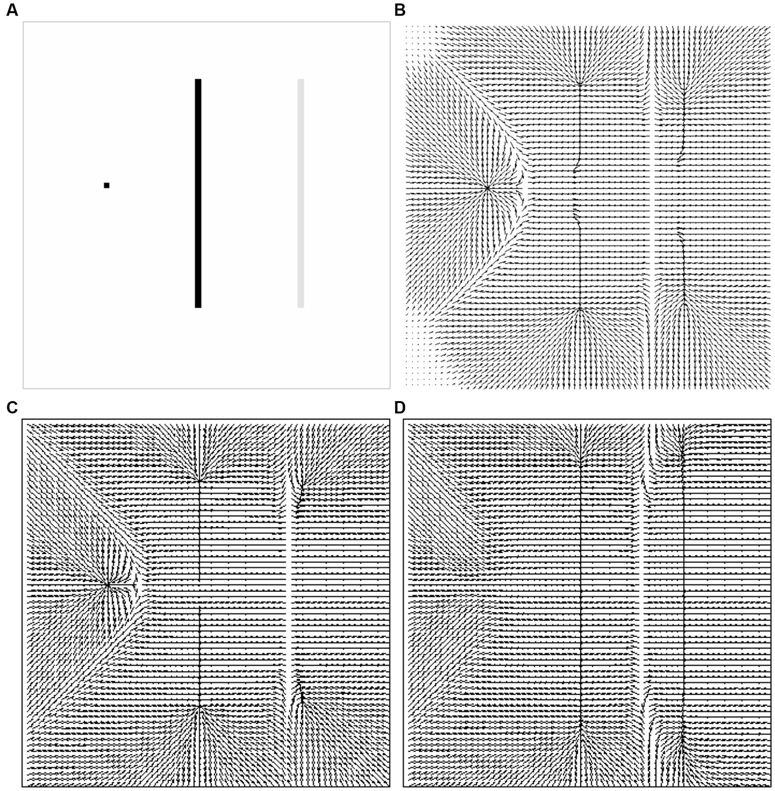
Figure 1. (A) Synthetic edge map including an impulse noise, a strong edge, and a weak edge. Vector fields of (B) GVF. (C) GGVF. (D) DWGVF.
3.3 Numerical implementation
One can get the solution of Eq. (12) by finding the equilibrium solution of the following PDEs in an iterative manner,
Taking as an example, the first and second derivatives of are calculated as follows,
where superscript n indicates the iteration number, and those for can be calculated in a similar way; Ix, Iy, fx, fy are not changed during iteration and can be discretized using the central difference scheme; for example, Ix, Iy are calculated as follows,
4 Experimental results
In this section, we will demonstrate some desirable properties of the DWGVF snake in terms of noise robustness, narrow and deep concavity convergence, weak edge preserving, and neighboring objects separation; the GVF (39) and GGVF (40) snakes are employed for comparison. All edge maps derived in this section are normalized to [0, 1]. The parameters for snakes in all experiments are and time step . Parameter μ for GVF is 0.2 in Figures 2, 3 to obtain a large capture range and 0.1 in Figures 4–9 for the sake of preserving edges. Parameter k acts as a threshold and controls the smoothing effect; according to the analysis in You and Xu (62), it should be slightly larger for heavy noise; as a result, for DWGVF and GGVF, it is 0.2 in Figures 2, 3, 0.08 in Figure 4, and 0.1 in Figures 5–7 for the sake of preserving weak edges; it is specifically configured for real medical images in Figures 8, 9.
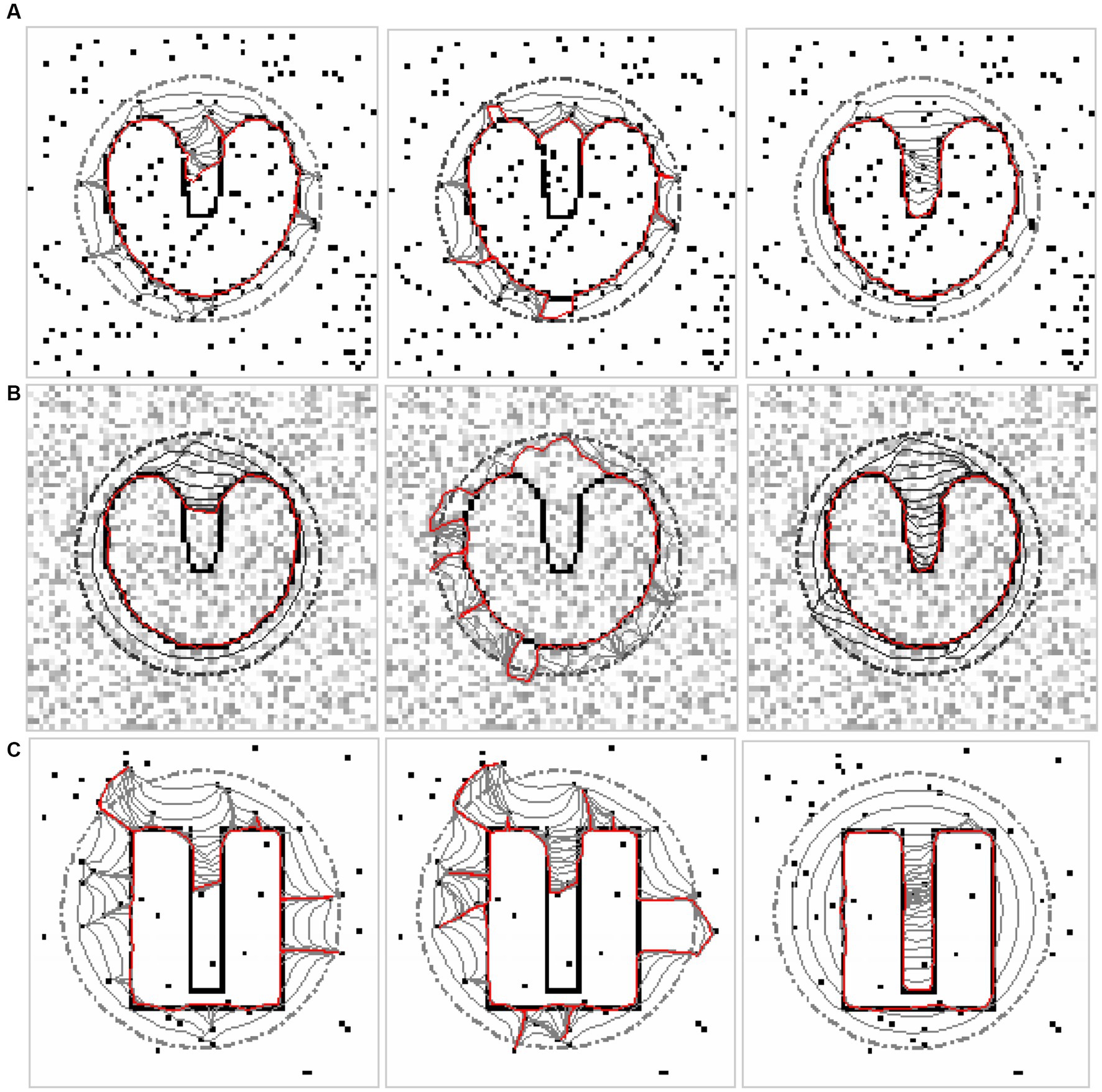
Figure 2. (A) U-shape image with salt and pepper noise. (B) U-shape image with speckle noise. (C) Deep concavity with salt and pepper noise. In each panel, the left is the convergence of the GVF snake, the middle is that of the GGVF snake, and the right is that of the DWGVF snake.

Figure 3. Evolutions and convergences to the deep concavity of (A) GVF snake, (B) GGVF snake, and (C) DWGVF snake.
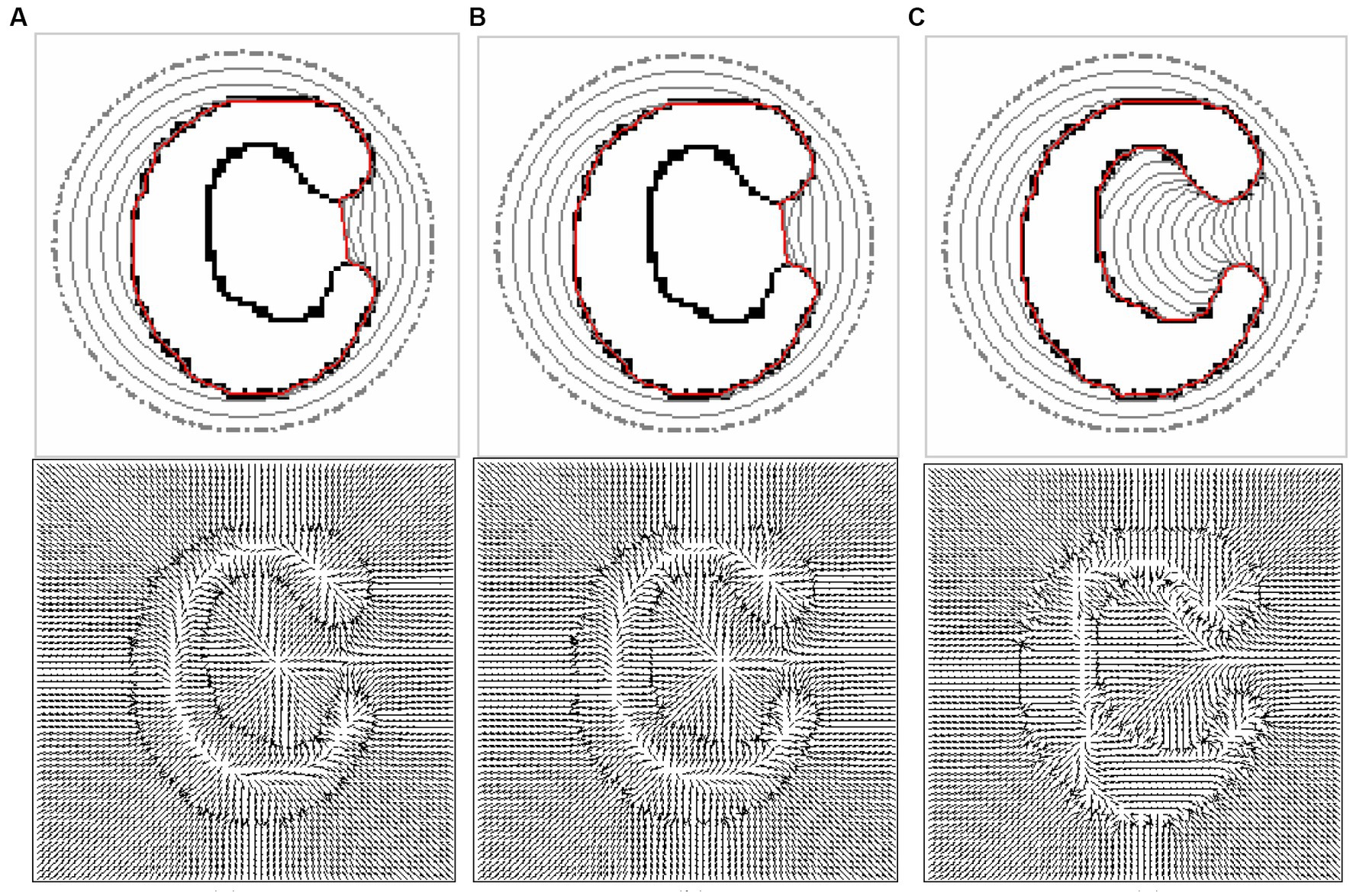
Figure 4. Performances of (A) GVF snake, (B) GGVF snake, and (C) DWGVF snake. In each panel, the upper is the evolution and convergence of the snake contour and the bottom is the corresponding force field.
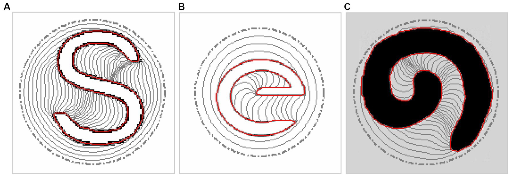
Figure 5. Evolutions and convergences of DWGVF snake to (A) S-shape, (B) e-shape, and (C) spiral shape concavities.
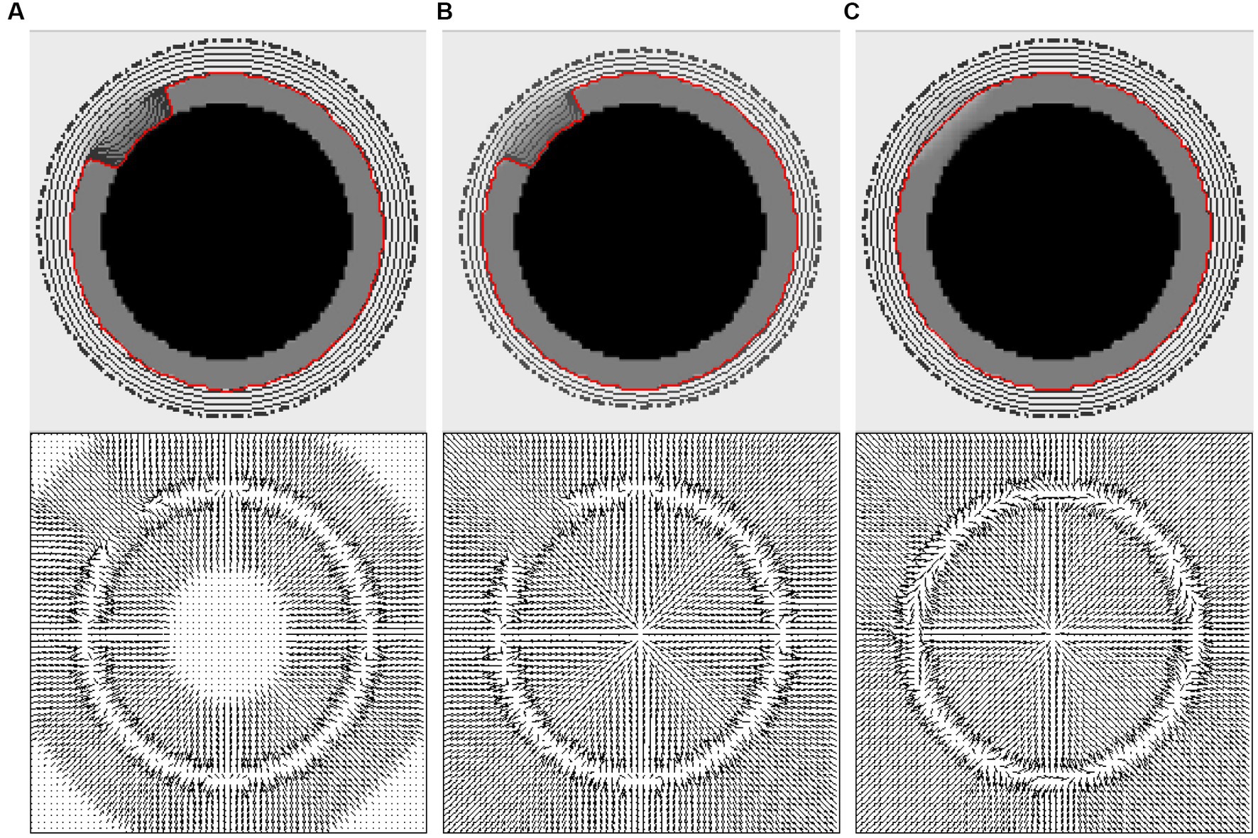
Figure 6. Performances of (A) GVF snake, (B) GGVF snake, and (C) DWGVF snake. In each panel, the upper is the evolution and convergence of the snake contour and the bottom is the corresponding force field.
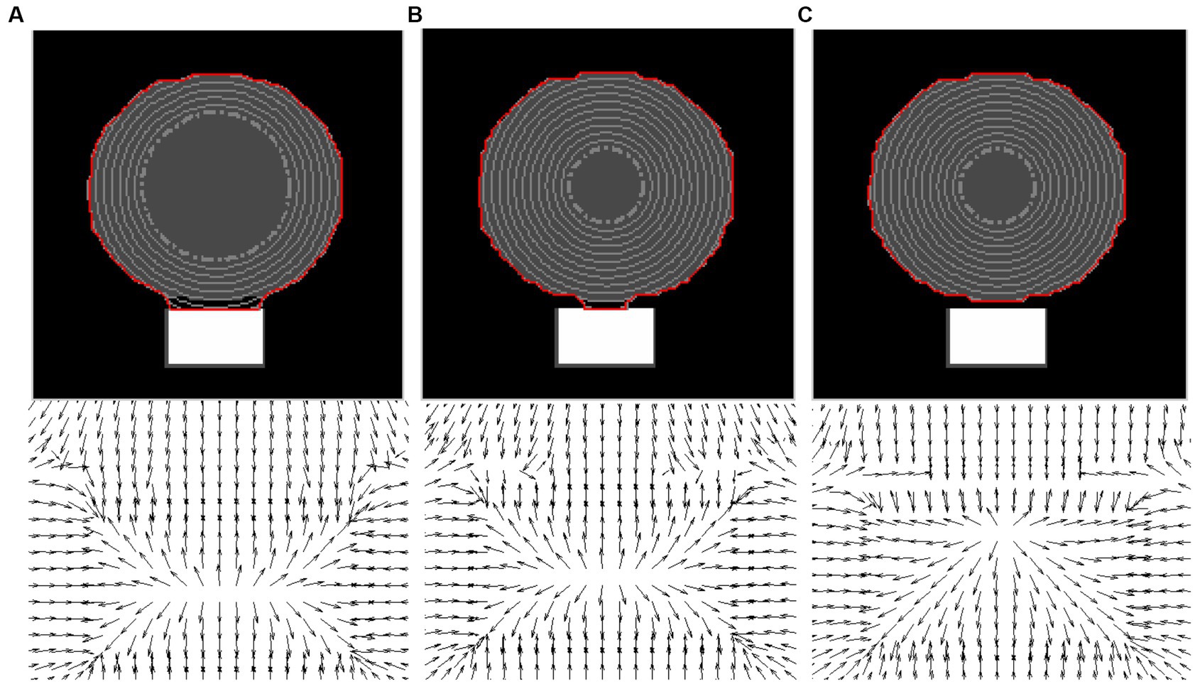
Figure 7. Performances of (A) GVF snake, (B) GGVF snake, and (C) DWGVF snake. In each panel, the upper is the evolution and convergence of the snake contour and the bottom is the close-up of the corresponding force field.
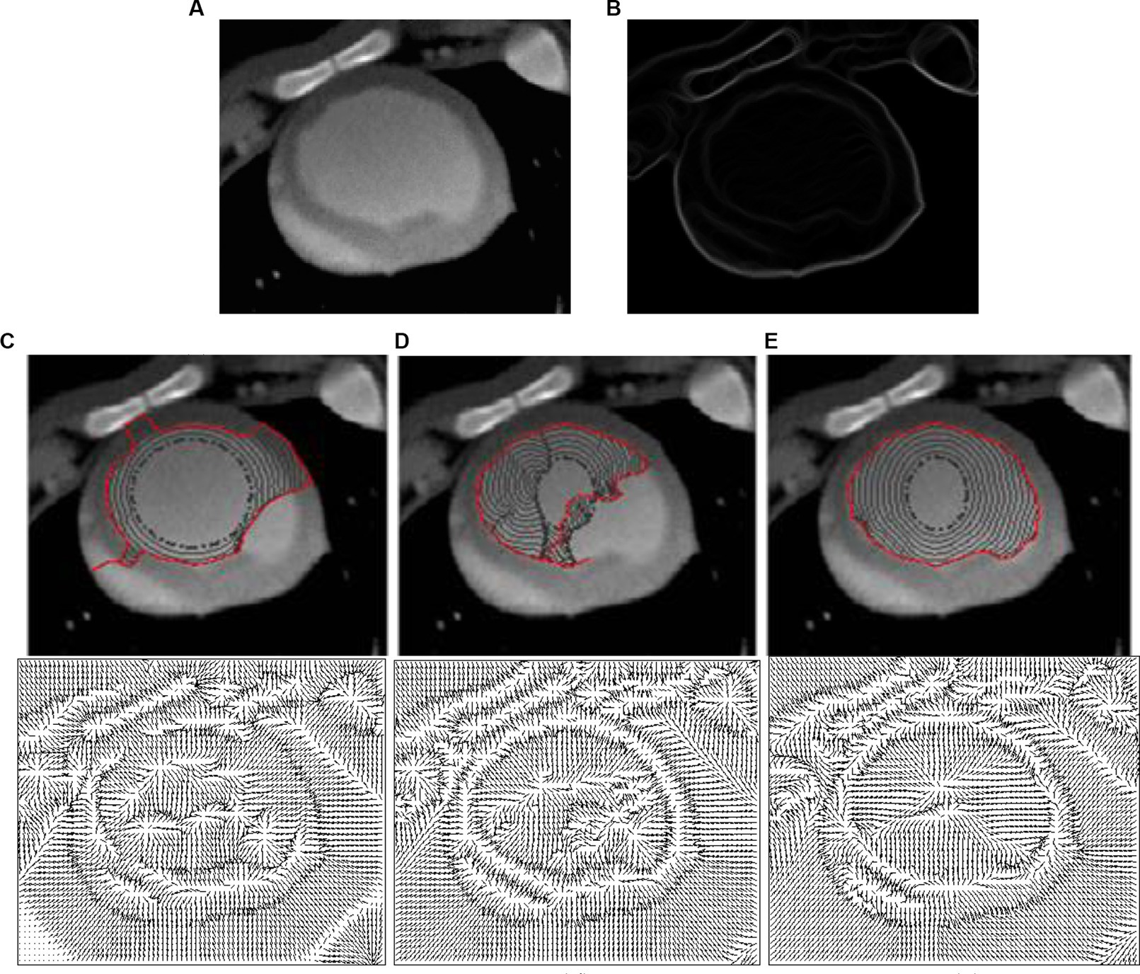
Figure 8. (A) Cardiac CT image. (B) Edge map. Performances of (C) GVF snake, (D) GGVF snake, and (E) DWGVF snake. In panels (C–E), the upper is the evolution and convergence of the snake contour and the bottom is the corresponding force field.
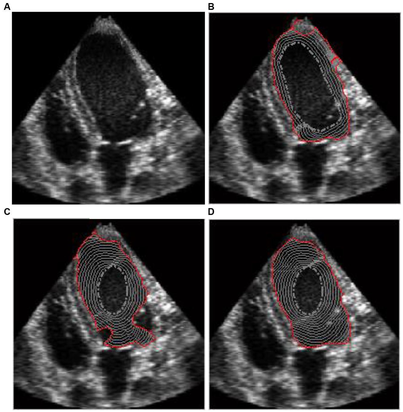
Figure 9. (A) Ultrasound heart image, evolutions, and convergences of (B) GVF snake, (C) GGVF snake, and (D) DWGVF snake.
4.1 Noise robustness
To demonstrate the noise robustness of the DWGVF snake, we employ the U-shape image, which was first introduced in Xu and Prince (39); however, in this subsection, it is contaminated by ‘salt and pepper’ noise and ‘speckle’ noise as shown in Figures 2A,B, respectively. Figure 2C presents another noisy image as an example with a concavity of 5 pixels wide and 30 pixels deep. The three noisy images are kept intact to calculate the GVF, GGVF, and DWGVF external forces. It can be seen from the results in Figure 2 that the proposed DWGVF snake could overcome the noise and converge to concavities successfully, whereas the GVF and GGVF snakes failed. The GGVF snake performs even worse as it is more sensitive to noise. In (39), the U-shape image with speckle noise was also employed to verify noise robustness of the GVF snake (see Figure 7 therein). However, the noisy U-shape image in Xu and Prince (39) is preprocessed with a Gaussian filter while the noisy image in our example is kept intact. Noise is usually unavoidable in applications, and noise insensitivity is a major concern in active contour-based image segmentation. The proposed DWGVF snake performs effectively and would be considerably beneficial to applications in this scenario.
4.2 Narrow and deep concavity convergence
It has been pointed out in Xu and Prince (40) that the GVF snake would fail to converge when the concavity is very narrow and very deep. Although the GGVF snake shows better performance than the GVF snake, when the concavity is deep enough, the GGVF snake still cannot converge. Figure 2C shows that the DWGVF snake can converge to a 5-pixel-wide and 30-pixel-deep indentation. What will happen if the concavity is narrower? Figure 3 shows the evolutions and convergences of GVF, GGVF, and DWGVF snakes on a 3-pixel-wide, 30-pixel-deep concavity. Even though there is no noise, the GGVF snake still fails to converge due to its isotropic nature. The result of the GVF snake is far from success, and only the DWGVF snake dives into concavity without hesitation. More satisfactory results have been achieved on much deeper concavities, but due to page limitations, the results are not presented here.
4.3 C-shape concavity convergence
U-shape concavity convergence is a difficult problem for classical snakes, but it can be easily handled in GVF-based snake models. Further studies show that the GVF and GGVF snakes cannot converge to C-shape concavity, see Figures 4A,B, respectively. C-shape concavity convergence is also important to many applications, but as far as we know, there is no GVF-based method aiming at this problem. The difference between U-shape and C-shape concavities is that the U-shape is open at the entrance while the C-shape is semi-close. Figure 4C shows the remarkable success of the proposed DWGVF snake in C-shape convergence.
The DWGVF snake is further applied to S-shape, e-shape, and spiral concavities, and the results are shown in Figure 5. These concavities are a little more complex than C-shape as there is orientation rotation, especially for e-shape and spiral concavities, whereas we can observe from Figure 5 the success of the DWGVF snake in extracting these concave boundaries.
4.4 Weak edge preserving and neighboring objects separation
The DWGVF snake also behaves well in weak edge preservation and neighboring objects separation, especially when the edge of one object is weak and that of the other is strong. This assertion is verified using two examples. One is a torus in Figure 6, but the upper left part of which is blurred and the edge of the outer circle is weak while that of the inner circle is strong. Neither the GVF snake nor the GGVF snake can correctly locate the outer circle. In contrast, the DWGVF snake shows satisfactory performance; see the results in Figure 6.
The other example is in Figure 7; there is one gray disk neighboring one white rectangle on a black background, and the spacing between the two objects is only three pixels. The boundary of the gray disk can be considered a weak edge while that of the rectangle is strong. Similar to the results in Figure 6, the failure of the GVF and GGVF snakes and the success of the DWGVF snake can be observed in Figure 7. The DWGVF snake outperforms the GVF and GGVF snakes once again. To note, Parameter k for DWGVF and GGVF is identical in these two examples.
4.5 Real images
After specific advantages of the DWGVF snake have been demonstrated on several synthetic images, it is further applied to real medical images. The first one is a cardiac CT image as shown in Figure 8A, and its edge map is shown in Figure 8B. Our purpose is to extract the endocardium of the left ventricle; to achieve this goal, we have to handle noise, inhomogeneity, and weak edges. Figures 8C,D shows that the GVF and GGVF snakes struggle with this case, whereas the DWGVF snake yields satisfactory result; see Figure 8E. Let us scrutinize the GVF, GGVF, and DWGVF fields at the bottom of Figures 8C–E one by one to further understand their behaviors. It is clear that the GVF is in disorder within the blood pool although weak edge leakage occurs. The GGVF succeeds in preserving weak edges by employing an appropriate k, but it is distracted by inhomogeneity within the blood pool. The DWGVF is smooth enough within the blood pool, and the weak edges are well preserved. We use k = 0.03 for GGVF and DWGVF in this example.
Another example in Figure 9A is an ultrasound heart image, and the purpose is also to extract the endocardium of the left ventricle. There remains a dilemma for the GVF and GGVF snakes to simultaneously preserve the weak edge and suppress the noise; therefore, the GVF snake leaks out at the weak edges (see Figure 9B) and the GGVF snake is blocked by the noise (see Figure 9C). However, the DWGVF snake yields a satisfactory compromise between noise suppression and weak edge preservation and locates the endocardium correctly with fairly far-off initialization (see Figure 9D). Parameter k is 0.06 for GGVF and DWGVF in this example.
5 Conclusion
In this study, a novel external force called directionally weakened gradient vector flow (DWGVF) for active contours has been proposed. The DWGVF method makes use of the image structure information of the original image by weakening the diffusion along the normal direction of the original image. The DWGVF also employs two spatiotemporally varying weights so that DWGVF is robust to noise. The DWGVF snake possesses some desirable properties of the GVF snake, such as large capture range and insensitivity to initialization. The DWGVF snake also shows high performance on noise resistance, concavity convergence, and weak edge preserving. The advantages of the DWGVF snake have been evaluated on both synthetic and real images, and comparisons with the GVF and GGVF snakes manifest that the DWGVF snake can serve as a superior alternative to the GVF and GGVF snakes.
In addition, the DWD diffusion can also be used for image restoration; this is a topic for future research.
Data availability statement
The original contributions presented in the study are included in the article/supplementary material, further inquiries can be directed to the corresponding authors.
Author contributions
ZW: Investigation, Software, Validation, Writing – original draft. NL: Funding acquisition, Methodology, Project administration, Validation, Visualization, Writing – review & editing. QZ: Conceptualization, Formal analysis, Resources, Writing – original draft. JW: Conceptualization, Data curation, Project administration, Supervision, Writing – original draft. LZ: Conceptualization, Supervision, and Project administration. YW: Conceptualization, Supervision, Writing – review & editing.
Funding
The author(s) declare financial support was received for the research, authorship, and/or publication of this article. This study was supported in part by the National Science Foundation of China (NSFC) under Grant No. 61976241 and in part by the International Science and Technology Cooperation Plan Project of Zhenjiang under Grant no. GJ2021008.
Acknowledgments
We acknowledge the National Science Foundation of China (NSFC) and the International Science and Technology Cooperation Plan Project of Zhenjiang for providing grants under Grant nos. 61976241 and GJ2021008, respectively.
Conflict of interest
The authors declare that the research was conducted in the absence of any commercial or financial relationships that could be construed as a potential conflict of interest.
Publisher’s note
All claims expressed in this article are solely those of the authors and do not necessarily represent those of their affiliated organizations, or those of the publisher, the editors and the reviewers. Any product that may be evaluated in this article, or claim that may be made by its manufacturer, is not guaranteed or endorsed by the publisher.
References
1. Kass, M, Witkin, A, and Terzopoulos, D (1988). Snake: active contour models. Int J Comput Vision 1:321–31. doi: 10.1007/BF00133570
2. Han, X, Xu, C, and Prince, J (2003). A topology preserving level set method for geometric deformable models. IEEE TPAMI 25:755–68. doi: 10.1109/TPAMI.2003.1201824
3. Wang, Y, Wang, H, and Xu, Y (2013). Texture segmentation using vector-valued Chan-Vese model driven by local histogram. Comput Electr Eng 39:1506–15. doi: 10.1016/j.compeleceng.2013.03.017
4. Yang, Y, Hou, X, and Ren, H (2022). Efficient active contour model for medical image segmentation and correction based on edge and region information. Expert Syst Appl 194:116436. doi: 10.1016/j.eswa.2021.116436
5. Zhu, SC, and Yuille, A (1996). Region competition: unifying snakes, region grouping, and Bayes/MDL for multiband image segmentation. IEEE TPAMI 18:884–900. doi: 10.1109/34.537343
6. Lie, J, Lysaker, M, and Tai, X-C (2006). A binary level set model and some applications to Mumford-Shah image segmentation. IEEE TIP 15:1171–81. doi: 10.1109/TIP.2005.863956
7. Cremers, D, Rousson, M, and Deriche, R (2007). A review of statistical approaches to level set segmentation: integrating color, texture, motion and shape. Int J Comput Vis 72:195–215. doi: 10.1007/s11263-006-8711-1
8. Vese, LA, and Chan, TF (2002). A multiphase level set framework for image segmentation using the Mumford–Shah model. IJCV 50:271–93. doi: 10.1023/A:1020874308076
9. Chan, TF, and Vese, LA (2001). Active contours without edges. IEEE TIP 10:266–77. doi: 10.1109/83.902291
10. Ayed, IB, Li, S, and Ross, I (2009). A statistical overlap prior for variational image segmentation. Int J Comput Vision 85:115–32. doi: 10.1007/s11263-009-0249-6
11. Li, CM, Kao, CY, Gore, JC, and Ding, ZH (2008). Minimization of region-scalable fitting energy for image segmentation. IEEE TIP 17:1940–9.
12. Brox, T, and Cremers, D (2009). On local region models and a statistical interpretation of the piecewise smooth Mumford-Shah functional. Int J Comput Vision 84:184–93. doi: 10.1007/s11263-008-0153-5
13. Lankton, S, and Tannenbaum, A (2008). Localizing region based active contours. IEEE TIP 17:2029–39.
14. Yang, Y, Wang, R, and Ren, H (2021). Active contour model based on local intensity fitting and atlas correcting information for medical image segmentation. Multimed Tools Appl 80:26493–509. doi: 10.1007/s11042-021-10890-4
15. Darolti, C, Mertins, A, Bodensteiner, C, and Hofmann, UG (2008). Local region descriptors for active contours evolution. IEEE TIP 17:2275–88.
16. Adam, A, Kimmel, R, and Rivlin, E (2009). On scene segmentation and histograms-based curve evolution. IEEE TPAMI 31:1708–14. doi: 10.1109/TPAMI.2009.21
17. Ni, K, Bresson, X, Chan, T, and Esedoglu, S (2009). Local histogram based segmentation using the Wasserstein distance. Int’l J. Computer Vision 84:97–111. doi: 10.1007/s11263-009-0234-0
18. Melonakos, J, Pichon, E, Angenent, S, and Tannenbaum, A (2008). Finsler active contours. IEEE TPAMI 30:412–23. doi: 10.1109/TPAMI.2007.70713
19. Sundaramoorthi, G, Yezzi, A, Mennucci, AC, and Sapiro, G (2009). New possibilities with Sobolev active contours. Int J Comput Vis 84:113–29. doi: 10.1007/s11263-008-0133-9
20. Weng, G, and Dong, B (2021). A new active contour model driven by pre-fitting bias field estimation and clustering technique for image segmentation. Eng Appl Artif Intell 104:104299. doi: 10.1016/j.engappai.2021.104299
21. Feng, B, Zhou, H, and Feng, J (2022). Active contour model of breast cancer DCE-MRI segmentation with an extreme learning machine and a fuzzy C-means cluster. IET Image Process 2022:12530. doi: 10.1049/ipr2.12530
22. Joshi, A, and Khan, MS (2021). Asim Niaz, active contour model with adaptive weighted function for robust image segmentation under biased conditions. Expert Syst Appl 175:114811. doi: 10.1016/j.eswa.2021.114811
23. Caselles, V, Kimmel, R, and Sapiro, G (1997). Geodesic active contours. Int J Comput Vis 22:61–79. doi: 10.1023/A:1007979827043
24. Paragios, N, Mellina-Gottardo, O, and Ramesh, V (2004). Gradient vector flow fast geometric active contours. IEEE TPAMI 26:402–7. doi: 10.1109/TPAMI.2004.1262337
25. Cohen, LD, and Cohen, I (1993). Finite-element methods for active contour models and balloons for 2-D and 3-D images. IEEE Trans Pattern Anal Mach Intell 15:1131–47. doi: 10.1109/34.244675
26. Mishra, A, and Wong, A (2010). KPAC: a kernel-based parametric active contour method for fast image segmentation. IEEE SP Letters 17:312–5. doi: 10.1109/LSP.2009.2036654
27. Srikrishnan, V, and Chaudhuri, S (2009). Stabilization of parametric active contours using a tangential redistribution term. IEEE TIP 18:1859–72.
28. Myronenko, A, and Song, XB. Global active contour-based image segmentation via probability alignment, CVPR2009. (2009).
29. Dong, B, Weng, G, and Jin, R (2021). Active contour model driven by self organizing maps for image segmentation. Expert Syst Appl 177:114948. doi: 10.1016/j.eswa.2021.114948
30. Fang, L, Liang, X, and Xu, C (2023). Image segmentation using a novel dual active contour model. Multimed Tools Appl 2023:15472. doi: 10.1007/s11042-023-15472-0
31. Zhou, S, Lu, Y, and Li, N (2019). Extension of the virtual electric field model using bilateral-like filter for active contours. SIViP 13:1131–9. doi: 10.1007/s11760-019-01456-x
32. Zhou, S, Li, B, and Wang, Y (2018). The line- and block-like structures extraction via ingenious Snake. Pattern Recogn. Lett. 112:324–31.
33. Wang, J, and Chan, KL (2015). Active contour with a tangential component. J Math Imaging Vis 51:229–47. doi: 10.1007/s10851-014-0519-y
34. Zhao, Chenji, Xiang, Shun, and Wang, Y., etc, Context-aware network fusing transformer and V-net for semi-supervised segmentation of 3D left atrium, Expert Syst Appl, 2023: 214:119105. doi: 10.1016/j.eswa.2022.119105
35. Zhang, H, Zhang, W, and Shen, W (2021). Automatic segmentation of the left ventricle from MR images based on nested U-net with dense block. Biomed Sig Proc Control 68:102684. doi: 10.1016/j.bspc.2021.102684
36. Shen, Weihao, Wenbo, Xu, and Sun, Zexin, etc, Automatic segmentation of the femur and tibia bones from X-ray images based on pure dilated residual U-net, Inverse Problems and Imaging, 2021, 15:1333–1346. doi: 10.3934/ipi.2020057
37. Wang, W, Wang, Y, and Wu, Y (2019). Quantification of full left ventricular metrics via deep regression learning with contour-guidance, IEEE. Access 7:47918–28. doi: 10.1109/ACCESS.2019.2907564
38. Antonelli, L, De Simone, V, and di Serafino, D (2022). A view of computational models for image segmentation. Ann Univ Ferrara 68:277–94. doi: 10.1007/s11565-022-00417-6
40. Xu, C, and Prince, JL (1998). Generalized gradient vector flow external forces for active contours. Signal Process 71:131–9. doi: 10.1016/S0165-1684(98)00140-6
41. Ray, N, and Acton, ST (2004). Motion gradient vector flow: an external force for tracking rolling leukocytes with shape and size constrained active contours. IEEE Trans Med Imaging 23:1466–78. doi: 10.1109/TMI.2004.835603
42. Wang, Y, Jia, Y, and Liu, L (2008). Harmonic gradient vector flow external force for snake model. IEE Electron Lett 44:105–7. doi: 10.1049/el:20081650
43. Cheng, J, and Foo, SW (2006). Dynamic directional gradient vector flow for snakes. IEEE Trans Image Process 15:1563–71. doi: 10.1109/TIP.2006.871140
44. Sum, KW, and Cheung, PYS (2007). Boundary vector field for parametric active contours. Pattern Recogn 40:1635–45. doi: 10.1016/j.patcog.2006.11.006
45. Tang, J (2009). A multi-direction GVF snake for the segmentation of skin cancer images. Pattern Recogn 42:1172–9. doi: 10.1016/j.patcog.2008.09.007
46. Ning Jifeng, W, Chengke, LS, and Shuqin, Y (2007). NGVF: an improved external force field for active contour mode. Pattern Recogn Lett 28:58–63. doi: 10.1016/j.patrec.2006.06.014
47. Li, C, Liu, CJ, and Fox, MD (2005). Segmentation of external force field for automatic initialization and splitting of snakes. Pattern Recogn 38:1947–60. doi: 10.1016/j.patcog.2004.12.015
48. Wang, Y, and Jia, Y. External force for active contours: gradient vector convolution. In: Pacific rim international conference on artificial intelligence(PRICAI), pp, 466–472. (2008).
49. Tauber, C, Batatia, H, and Ayache, A (2010). Quasi-automatic initialization for parametric active contours. Pattern Recogn Lett 31:83–90. doi: 10.1016/j.patrec.2009.08.010
50. Park, HK, and Chung, MJ (2002). External force of snake: virtual electric field. Electron Lett 38:1500–2. doi: 10.1049/el:20021037
51. Wang, Y, Liu, L, Zhang, H, Cao, Z, and Lu, S (2010). Image segmentation using active contours with normally biased GVF external force. IEEE Sig Proc Lett 17:875–8. doi: 10.1109/LSP.2010.2060482
52. Jaouen, V, González, P, and Stute, S (2014). Variational segmentation of vector-valued images with gradient vector flow. IEEE TIP 23:4773–85. doi: 10.1109/TIP.2014.2353854
53. Zhang, Z, Duan, C, and Lin, T (2020). Etc, GVFOM: a novel external force for active contour based image segmentation. Inf Sci 506:1–18. doi: 10.1016/j.ins.2019.08.003
54. Yu, H, and Chua, CS (2006). GVF-based anisotropic diffusion models. IEEE Trans Image Process 15:1517–24. doi: 10.1109/TIP.2006.871143
55. Prasad, VSN, and Yegnanarayana, B (2004). Finding axes of symmetry from potential fields. IEEE Trans Image Process 13:1559–66. doi: 10.1109/TIP.2004.837564
56. Hassouna, MS, and Farag, AA (2009). Variational curve skeletons using gradient vector flow. IEEE TPAMI 31:2257–74. doi: 10.1109/TPAMI.2008.271
57. Bai, J, Shah, A, and Xiaodong, W (2018). Optimal multi-object segmentation with novel gradient vector flow based shape priors. Comput Med Imaging Graph 69:96–111. doi: 10.1016/j.compmedimag.2018.08.004
58. Jaouen, V, Bert, J, and Boussion, N (2018). Etc, image enhancement with PDEs and nonconservative advection flow fields. EEE Trans Image Proc 2018:1838. doi: 10.1109/TIP.2018.2881838
59. Van Dang, L, and Makhanov, S (2020). Enhanced vector flow of significant directions for five-axis machining of STL surfaces. Int J Prod Res 59:3664–95. doi: 10.1080/00207543.2020.1749325
60. Nagel, HH (1987). On the estimation of optical flow: relations between different approaches and some new results. Artif Intell 33:299–324. doi: 10.1016/0004-3702(87)90041-5
61. Kuijper, A (2009). Geometrical PDEs based on second order derivatives of gauge coordinates in image processing. Image Vis Comput 27:1023–34. doi: 10.1016/j.imavis.2008.09.003
62. You, Y, Xu, W, Tannenbaum, A, and Kaveh, M (1996). Behavioral analysis of anisotropic diffusion in image processing. IEEE TIP 5:1539–52.
Keywords: image segmentation, active contours, gradient vector flow, directionally weakened diffusion, second directional derivative
Citation: Wang Z, Li N, Zhang Q, Wei J, Zhang L and Wang Y (2023) Directionally weakened diffusion for image segmentation using active contours. Front. Appl. Math. Stat. 9:1275588. doi: 10.3389/fams.2023.1275588
Edited by:
Qiyu Jin, Inner Mongolia University, ChinaReviewed by:
Zhifeng Pang, Henan University, ChinaLaura Antonelli, National Research Council (CNR), Italy
Yunjie Chen, Nanjing University of Information Science and Technology, China
Chaofeng Li, Shanghai Maritime University, China
Copyright © 2023 Wang, Li, Zhang, Wei, Zhang and Wang. This is an open-access article distributed under the terms of the Creative Commons Attribution License (CC BY). The use, distribution or reproduction in other forums is permitted, provided the original author(s) and the copyright owner(s) are credited and that the original publication in this journal is cited, in accordance with accepted academic practice. No use, distribution or reproduction is permitted which does not comply with these terms.
*Correspondence: Yuanquan Wang, d2FuZ3l1YW5xdWFuQHNjc2UuaGVidXQuZWR1LmNu; Jin Wei, d2o5NzE3QHNpbmEuY29t; Lei Zhang, emhhbmdsZWlAaGVidXQuZWR1LmNu
†These authors have contributed equally to this work