Simulating time-to-event data under the Cox proportional hazards model: assessing the performance of the non-parametric Flexible Hazards Method

Numerous methods and approaches have been developed for generating time-to-event data from the Cox Proportional Hazards (CPH) model; however, they often require specification of a parametric distribution for the baseline hazard even though the CPH model itself makes no assumptions on the distribution of the baseline hazards. In line with the semi-parametric nature of the CPH model, a recently proposed method called the Flexible Hazards Method generates time-to-event data from a CPH model using a non-parametric baseline hazard function. While the initial results of this method are promising, it has not yet been comprehensively assessed with increasing covariates or against data generated under parametric baseline hazards. To fill this gap, we conducted a comprehensive study to benchmark the performance of the Flexible Hazards Method for generating data from a CPH model against parametric methods. Our results showed that with a single covariate and large enough assumed maximum time, the bias in the Flexible Hazards Method is 0.02 (with respect to the log hazard ratio) with a 95% confidence interval having coverage of 84.4%. This bias increases to 0.054 when there are 10 covariates under the same settings and the coverage of the 95% confidence interval decreases to 46.7%. In this paper, we explain the plausible reasons for this observed increase in bias and decrease in coverage as the number of covariates are increased, both empirically and theoretically, and provide readers and potential users of this method with some suggestions on how to best address these issues. In summary, the Flexible Hazards Method performs well when there are few covariates and the user wishes to simulate data from a non-parametric baseline hazard.

1. Introduction

Survival analysis refers to a class of statistical procedures for analyzing data where the variable of interest is the time until the occurrence of an event of interest. Time-to-event data is common across a broad range of disciplines, particularly biomedical research [1, 2]. As an example, consider a lung cancer clinical trial where 164 patients with non-small cell lung cancer randomly received one of two different treatments. The time until the first relapse for each individual was recorded and these data were analyzed to see if one treatment was more effective at preventing or delaying relapse than the other [3]. One of the most frequently used models to analyze such data is the Cox Proportional Hazards (CPH) model, which takes on the following general form in Equation 1.

$\begin{array}{ll}\begin{array}{l}{h}_i(t)=h_0(t)exp({\text{X}}_{\text{i}}\beta )\end{array}& (1)\end{array}$

In this equation, the expected individual hazard function, h_i(t), is the probability that an individual experiences the event at time t; h₀(t) is the baseline hazard which represents the hazard when all X_i are equal to 0; X_i is a p-dimensional vector of covariates for the i^th individual, i =1,…, n; and β is a vector of model parameters of length p. The expected individual hazard is the product of the baseline hazard and the exponential function of the linear predictors, which means that the predictors have a multiplicative or proportional effect on the expected hazard from one instance in time to the next. Further, when comparing the expected hazards of two individuals (i and j), the ratio of their respective hazards can be taken as in Equation 2.

$\begin{array}{ll}\begin{array}{l}\frac{h_0(t)exp({\text{X}}_{\text{i}}\beta )}{h_0(t)exp({\text{X}}_{\text{j}}\beta )}=exp({\text{X}}_{\text{i}}\beta -{\text{X}}_{\text{j}}\beta )\end{array}& (2)\end{array}$

Since this hazard ratio does not depend on time, t, the hazard is proportional over time. Moreover, since the hazard does not need to be specified in order to estimate the model parameters, β, a partial likelihood method is used. Suppose we have paired survival time and censoring indicators (t_i, δ_i) for an individual as well as fixed covariates X_i. An individual is censored δ_i ∈ {0, 1} when the true survival time, t_i, for that individual is unknown. Some examples of censoring include losing an individual in a study due to follow-up or an individual survives past the end of the study. Assuming there are no tied event times, a set D = {i | δ_i = 1} is defined where D is a set of those individuals that experience the event of interest. Further, the risk set, or the set of individuals at risk at time t is defined as R(t) = {i | t_i ≥ t}. The partial likelihood for the CPH model is displayed in Equation 3:

$\begin{array}{ll}\begin{array}{c}L(\beta )={\displaystyle {\prod }_i}\frac{P(T_i|T_i\ge t_i)}{{\displaystyle {\sum }_{k:t_k\ge t_i}}P(T_k=T_k|T_k\ge T_i)}={\displaystyle {\prod }_i}\frac{h_i(t_i)}{{\displaystyle {\sum }_{k:t_k\ge t_i}}{h}_k(t_k)}\\ ={\displaystyle {\prod }_i}\frac{exp({\text{X}}_{\text{i}}\beta )}{{\displaystyle {\sum }_{k:t_k\ge t_i}}exp({\text{X}}_{\text{k}}\beta )}\end{array}& (3)\end{array}$

In the above methodology, it is assumed there are no tied event times. In order to account for tied event times, the partial likelihood can be redefined to account for ties. One common method to account for ties was introduced by Breslow [4]. Contrary to estimating the Cox model using the method of partial likelihood with an existing dataset, when simulating time-to-event data from the semi-parametric CPH model, the baseline hazard must either be specified or a suitable non-parametric method must be used to generate baseline hazard. Cox and Therneau and Grambsch are resources for the reader to take a deeper look into the derivation of the CPH model [5, 6].

Simulating data from a statistical model is an important exercise as it allows one to understand robustness of a given model under misspecification and/or violations of its underlying assumptions, can facilitate comparisons of different analytical approaches or models under controlled conditions, and is useful for simulation-based assessments of statistical power. In the current literature, the baseline hazard is nearly always specified using a parametric distribution where the parameters in the distribution are chosen arbitrarily or set based on estimated parameter values from pilot studies. Common baseline hazard distributions used in the literature include the Weibull, exponential, log-normal, and gompertz distribution all of which satisfy the proportional hazards assumption [7–9]. There are many well-defined packages available in the R statistical programming language for generating time-to-event data from the CPH model when the baseline hazards is assumed to have a specific parametric form. This includes the survsim package and flexsurv, the latter of which is capable of fitting even more flexible parametric distributions [10, 11]. The use of these distributions has been extended to include methods for generating survival times with time-invariant covariates as well as cyclic and piecewise time-varying covariate [12]. Current research is being conducted for the generation of right-censored survival times as a function of time-varying covariates [13–15]. Some of these recent works consider Zhou's method for generating right-censored data for a functional form covariate using a piecewise exponential framework [16]. Hendry furthers Zhou's method by developing an algorithm to generate right-censored survival data with both time-invariant and time-varying covariates that vary at integer-valued steps on a time scale under the Cox model [13]. Other recent work demonstrates that the Lambert W Function can be used to generate survival times with time-varying covariates and derives closed-form solutions when the survival times follow an Exponential or a Weibull distribution [15]. Nevertheless, these methods still assume the survival times to have a specific parametric distribution even though in practice these distributions and subsequent parameter values are often unknown making simulations and the evaluation of analytical methods quite difficult and sometimes unrealistic. To date, there are relatively few studies that have focused on simulating data from a non-parametric baseline hazard, taking advantage of the flexible nature of the semi-parametric framework of the Cox model.

Previously developed methods for estimating a non-parametric baseline hazard include using a kernel-based approach with global and local bandwidth selection algorithms [17], a nearest-neighbor bandwidth approach [18], or spline-based estimators [19]. A simulation study was conducted by Hess et al. to compare the statistical properties of some of these earlier kernel-based methods [20]; in 2010, Hess et al. developed the corresponding R package, muhaz, which implements the boundary kernel formulations from Müller and the nearest neighbor bandwidth formulation from Gefeller and Dette [21]. This methodology and the resulting R package cannot handle covariates within its model framework, but it does have an advantage over some other methods that require the specification of complex nuisance model parameters, parameters which directly affect the estimates of the parameters of interest. A more recent method for estimating the non-parametric baseline hazard uses b-splines, implemented in the R-package, bshazard [22]. This method assumes that survival data already exist and does not allow simulation of data directly from the estimated baseline hazard. It also allows for the use of covariates, although the authors caution using covariates when estimating the baseline hazard due to the assumption that the covariates have a constant effect on the proportional hazards. The Flexible Hazards Method proposed by Harden and Kropko is capable of simulating time-to-event data without providing any of the survival data for the individuals using a non-parametric baseline hazard [23]. The Flexible Hazards Method can be implemented using sim.survdata function contained within the coxed R package [24]. The sim.survdata function is user-friendly and can accept user-specified coefficients, covariates, and can facilitate the generation of time-to-event data with time-varying covariates or using time-varying coefficients. To the best of our knowledge, the method proposed by Harden and Kropko is one of only few readily available methods with an existing easy-to-implement R package that allows for the simulation of time-to-event data under the Cox model while using a non-parametric method that allows for multiple covariates and does not rely on a pre-existing dataset.

While the Flexible Hazards Method is conceptually simple and easy to implement using the sim.survdata function, and has the distinct advantage that the user does not have to specify a distribution for the baseline hazard function, we have noticed that issues arise when the number of predictor variables (e.g., number of elements in X_i) are increased [23]. Specifically, unless careful attention is given with respect to how the elements of X_i are generated as well as the magnitude of the effect-size, β, e.g., log-hazard ratio parameters, as the dimension of X_i grows, so too does the magnitude of bias in the estimates of β obtained from Cox proportional hazards models obtained fit to the simulated data. Following from this observation, the purpose of this study is three-fold: (1) to illustrate this phenomenon in the increase in the magnitude of the bias with increasing number of parameters, (2) explain the plausible reasons for such, both empirically and theoretically, and (3) provide readers and potential users of the Flexible Hazards Method with suggestions on how to best address this issue. In what follows, we begin by describing the Flexible Hazards Method, followed by a description a series of simulation studies that were conducted to address the previously stated goals.

2. Methods

2.1. Simulating time-to-event data from the Flexible Hazard method

Here, we briefly describe the Flexible Hazards Method and refer readers to the original paper for a more complete description [23]. To simulate time-to-event data under the CPH model, a failure cumulative distribution function (CDF) is first generated. The failure CDF is generated by creating a time index of length T, where T can be interpreted as the maximum follow-up time for the study being simulated. Next, k-2 points, where k < < T, are randomly drawn from a Uniform(0, T) distribution, with the remaining two points being set to 0 and T. The result is a vector t of length k, whose elements, 0 ≤ t_r ≤ T, r = 1, 2, …, k. The cumulative probability of failure index is then generated by randomly drawing k-2 points form a Uniform(0,1) distribution, sorted in ascending order to ensure that the CDF is non-decreasing. The first point is set to 0 at the minimum time and the last point is set to 1 at the maximum time, T. The cumulative probability of failure is then visualized as a function of time on a graph (Figure 1A). Next, a cubic smoothing spline with third order polynomials is fit to these random points (Figure 1B). The probability distribution function (Figure 1C) is then retrieved by computing the first differences of the failure CDF at each time point since the failure CDF curve is the area under the PDF. We can also think about this in terms of differentiating the CDF to get the PDF. The baseline survival function and baseline hazard follow the general formulas where the baseline survival function is simply one minus the Failure CDF (Figure 1D) and the baseline hazard is the PDF divided by the survival function (Figure 1E). Using the calculated baseline survival function, S₀(t), the survival function for subject i, S_i(t), is given by Equation 4.

$\begin{array}{ll}\begin{array}{l}{S}_i(t)=S_0{(t)}^{exp\{{\text{X}}_i\beta \}}\end{array}& (4)\end{array}$

where β is the vector of parameters (e.g., log hazard ratios) and X_i is a vector of covariates for the i^th individual. As indicated by Equation (1), when exp{X_iβ} = 1.0, S_i(t) = S₀(t), whereas when exp{X_iβ} = 1.25, the risk of failure at time t conditional on survival through time t, is 25% higher than the baseline. To get the survival time for individual i, a single value from a Uniform(0,1) distribution is first drawn. Using the sampled value and the plot of survival as a function of time with a horizontal line extending from the sampled value, one then determines where the horizontal line intersects with S_i(t). The t at which this horizontal line intersects with S_i(t) is taken to be the survival time for individual i (Figure 1F). Once survival times for every individual i = 1,2,…,N have been determined, censoring is randomly assigned based upon a pre-specified censoring rate.

FIGURE 1

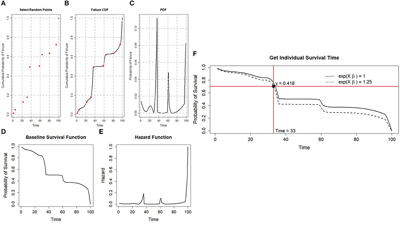
Figure 1. The Flexible Hazards methodology. This figure depicts the Flexible Hazards Method when T = 100 and k = 10. (A) (top left): k-2 = 8 randomly graphed points for both time and the cumulative probability of failure. (B) (top middle): A cubic spline fit through the randomly generated points from (A). (C) (top right): The PDF transformed by taking the first differences of the CDF in (B) at each time point. (D) (bottom left): The generated baseline survival function found by taking 1-CDF. (E) (bottom right): The generated hazard function (PDF divided by the survival function). (F) (right): The baseline survival function displayed with a solid black line and an individual's survival function where exp(Xβ) = 1.25 displayed by a dashed line. The randomly drawn uniform (0,1) point was 0.418 and this intersected the individual's survival function at time 33.

2.2. Simulation studies and generation of time-to-event data from parametric distributions

We conducted a series of simulation studies to comprehensively examine the Flexible Hazard Method. A description of the settings for our simulation studies are summarized in Table 1. Briefly, to simulate data using the Flexible Hazard Method, we start by setting the total sample size (n ∈ {1,000; 10,000}) and the number of variables to be included in the CPH model (p ∈ {1, 5, 10}). Next, we generate the covariate data, X_ij, i = 1,2,…, n and j = 1,2,…, p for each of the variables that will be included in the CPH model by randomly sampling from a multivariate normal distribution with mean-vector of 0 and variance-covariance matrix equal to the identity matrix. We then set the T index to be either 100, 500, or 1,000. The true parameter values, β_j, j = 1,…, p, are randomly drawn from a Uniform(−1,1) distribution. Next, we applied the sim.survdata function based on each combination of the simulation parameters described in Table 1. Specifically, in the sim.survdata function, argument “T” was specified to be the value of the T index, “X” was specified to be the simulated covariate data X, “beta” was set to the randomly generated true parameter values β, “censor” was set to the considered censoring rates (Table 1), the “fixed.hazard” option was set to FALSE, and “num.data.frames” was set to 1. The output of the sim.survdata function are simulated survival times and censoring indicators, generated based on the Flexible Hazards Method, for each of the n individuals. The simulated event times and covariate data X were then used in fitting a multivariable CPH model using the coxph function in the survival R package, where tied event-times were addressed using the Efron method [25].

TABLE 1

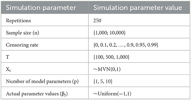
Table 1. Summary of the parameters assumed for the simulation study.

To benchmark the performance of the flexible hazard method, we used the inverse CDF method to generate time-to-event data, assuming both Weibull and exponential baseline hazard distributions. Specifically, time-to-event data were generated as follows in Equations 5, 6.

$\begin{array}{ll}\begin{array}{l}Exponential:t=\frac{-log(U)}{\lambda \times exp(\beta \text{X})}\end{array}& (5)\end{array}$

$\begin{array}{ll}\begin{array}{l}Weibull:t={\left(\frac{-log(U)}{\lambda \times exp(\beta \text{X})}\right)}^{-\gamma }\end{array}& (6)\end{array}$

In Equations 5, 6, t represents the survival time, U is a random draw from a Uniform(0,1) distribution, β is the vector of true parameter values drawn from the Uniform (-1,1) distribution, and X is the n x p matrix of randomly drawn covariate values. To enable fair comparisons, it is noted that the same linear predictors, βX, that were randomly generated for use in generating time-to-event data via the Flexible Hazard Method described above, were also used when generating time-to-event data assuming Weibull and exponential distribution for the baseline hazards. The nuisance parameters, λ and γ, for generating the survival times were arbitrarily set as they were not of direct interest in our simulation study. For our simulations, the nuisance parameter λ was set to 0.5 and γ was set to 1.5. The censoring indicator was then assigned by n random draws from a binomial distribution with probability equal to the assigned censoring rate. As was the case for time-to-event data generated using the Flexible Hazards Method via the sim.survdata function, survival times generated assuming Weibull and exponential distributions for the baseline hazard, were used in fitting a multivariable CPH model using the coxph function within the survival R package [26].

2.3. Performance assessment

For each of the three different assumptions of the baseline hazard—exponential, Weibull, and the Flexible Hazards Method, a CPH model was fit to the resulting data using the methodology described above. Based on the model fit, we compared the true parameter coefficients (β_j) with those estimated from the CPH model (${\widehat{\beta }}_j$) and computed the absolute bias for the j^th parameter as follows in Equation 7,

$\begin{array}{ll}\begin{array}{l}Bia{s}_j=|{\beta }_j-{\widehat{\beta }}_j|\end{array}& (7)\end{array}$

Along with the bias, we also calculated the coverage by computing the fraction of simulated data sets where the 95% confidence interval for a given model parameter contained the true parameter value. This process was repeated for 250 Monte Carlo (MC) simulations for each simulation setting in Table 1. When more than one parameter existed, the average bias and average coverage for all model parameters was calculated. This average was then the value for that one iteration of the 250 iterations. Once all iterations were completed, averages and confidence intervals were then computed for both the bias and the coverage using all 250 iterations.

3. Results

A series of simulation studies were used to evaluate the performance of the Flexible Hazards Method when the number of covariates associated with the risk of the event is increased. The performance of the flexible hazard method was then compared to two commonly assumed distributions for the baseline hazard function, the Weibull and exponential, as the number of covariates were increased. The results section is organized in three subsections. In the first subsection, we report the results comparing the Flexible Hazards Method against Weibull and exponential approaches when p = 1. Next, we report the results from the same comparison when p is increased, p > 1. Finally, we report results comparing the performance differences of the flexible hazard method to the parametric distributions when p = 1 to p > 1 as a means toward highlighting probable reasons for such differences.

3.1. A single covariate

When a single covariate is assumed to associate with the risk of the event, p = 1, the average absolute bias observed for the Flexible Hazards Method is comparable to what was observed when time-to-event data were generated assuming exponential and Weibull distributions for the baseline hazard function. When p = 1 and at maximum follow-up time of 1,000, T = 1,000, the average absolute bias for the flexible hazard method is 0.018 with the inter-quartile range (0.008, 0.031). Similarly, the average absolute bias and inter-quartile range for the exponential and Weibull parametric distributions was 0.015 (0.007, 0.025) and 0.015 (0.007, 0.026), respectively. Here, the bias is being computed by taking the absolute difference in the log of the hazard ratio (the coefficient value received from the coxph() model) and the true parameter value. Once all Monte Carlo simulations have been completed, the bias calculated at each iteration are then averaged and the inter-quartile range is computed. Ideally, the bias should be close to 0. Table 2 shows the results of the average absolute bias and Table 3 shows the average coverage when the maximum follow-up time for the Flexible Hazards Method, T, is increased from 100 to 1,000. The maximum follow-up time for both the exponential and Weibull distribution is infinity, based on the support of these distributions, and the small variation in these rows (rows 1, 4, and 7 from Tables 2, 3 where p = 1 for the Exponential and Weibull distribution columns) is simply due to variations in samples from the 250 MC iterations. From Tables 2, 3, we see that as T is increased, the average absolute bias observed for the Flexible Hazards Method is very similar to its parametric counterparts when p = 1. The coverage of the true parameter value also behaves similarly. As T is increased, the coverage of the Flexible Hazards Method increases from 0.588 to 0.844; whereas, the coverage for both the Weibull and exponential distributions are near 0.95. The coverage is being calculated by calculating the fraction of times the 95% confidence interval contains the true parameter value across all Monte Carlo repetitions. We expect, then, the coverage to be at or near 0.95. It is noted that in the following results, the sample size of n = 10,000 is displayed. The reader is referred to Supplementary Table 1 for the results of the average absolute bias and Supplementary Table 2 for the results of the average coverage when the sample size is n = 1,000.

TABLE 2

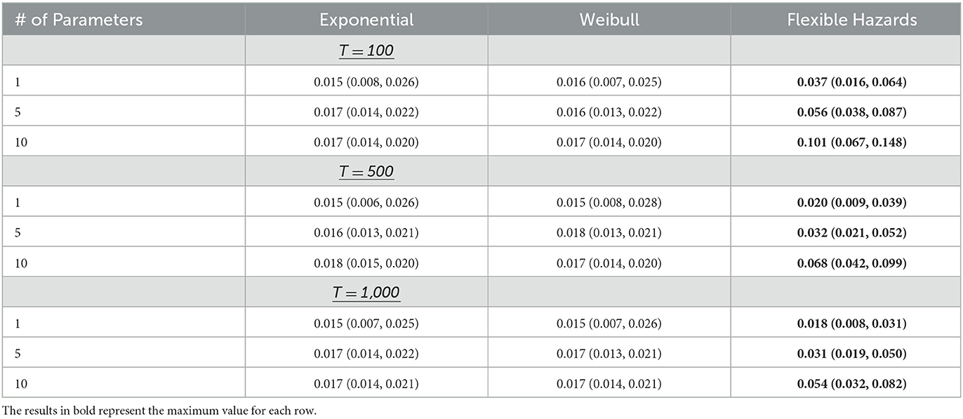
Table 2. The median (IQR) absolute bias in the parameter estimates for the exponential, Weibull, and Flexible Hazards Method across all simulated maximum event times for the Flexible Hazards Method with n = 10,000.

TABLE 3

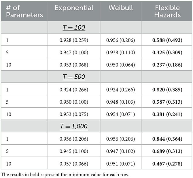
Table 3. The average coverage (standard deviation) in the parameter estimates for the exponential, Weibull, and Flexible Hazards Method across all simulated maximum event times for the Flexible Hazards Method with n = 10,000.

3.2. More than one covariate

Table 2 shows the results when n = 10,000 for the average absolute bias and Table 3 shoes the average coverage when p is increased to 5 or 10 covariates associated with the risk of the event, p ∈ {5,10} with increasing maximum follow-up time for the Flexible Hazards Method, T ∈ {100, 500, 1,000}. From this table we see that as T is increased, the mean absolute bias of the flexible hazard method does decrease, however it does not perform as well as the exponential and Weibull distributions. The average absolute bias also increases as p is increased. For p = 5 and T = 1,000, the Flexible Hazards Method has a mean absolute bias of 0.031; whereas the average absolute bias for the exponential and Weibull distributions were both 0.017. The average coverage of the true parameter value is 0.689 compared to 0.95 for the exponential and Weibull distributions. When p is further increased to 10, p = 10, at T = 1,000, the Flexible Hazards Method had a mean absolute bias of 0.054, whereas the average absolute bias observed form the exponential and Weibull distributions was 0.017, for both. The average coverage for p = 10 and T = 1,000 is only 0.467 for the Flexible Hazards Method compared to approximately 0.95 for the exponential and Weibull distributions. Thus, while the performance of the exponential and Weibull distributions appears to be invariant to increasing p, we observe a notable drop-off in the performance of the Flexible Hazards Method in terms of the mean absolute bias and average coverage as p is increased. The reader is referred to Supplementary Table 1 for the results of the average absolute bias and Supplementary Table 2 for the results of the average coverage when the sample size was lowered to n = 1,000.

3.3. Discrepancy in performance of Flexible Hazards Method with increasing p

With regard to the Flexible Hazards Method, we observed that the mean absolute bias increases proportionally for increasing p, whereas the mean absolute bias of the exponential and Weibull distributions remains constant even with the increase in parameters. One plausible explanation for the increase in the mean absolute bias observed for the Flexible Hazards Method with increasing p is that as p is increased, the number of individuals having tied event times also increases. Specifically, the number of individuals having the minimum or maximum event time, T, increases. Figure 2 shows scatterplots comparing the number of samples that have a maximum event time, T, to the mean absolute bias for increasing p. From this figure, we see that when there is only a single covariate, the pairwise Spearman correlation is 0.42 between the number of samples at the maximum event time and the mean absolute bias. This correlation increases to 0.91 when there are 9 parameters associated to the event of interest. In order to investigate how the increase in tied maximum event times affects the mean absolute bias, an additional set of simulations were conducted. These simulations were conducted based on the number of individuals with an event time exactly equal to the maximum event time that were generated using the Flexible Hazards Method. We then constrained data generated using the exponential and Weibull baseline hazards to have the same number of individuals with event times occurring at the maximum event time. A conceptual overview of how this was accomplished is given in Figure 3.

FIGURE 2

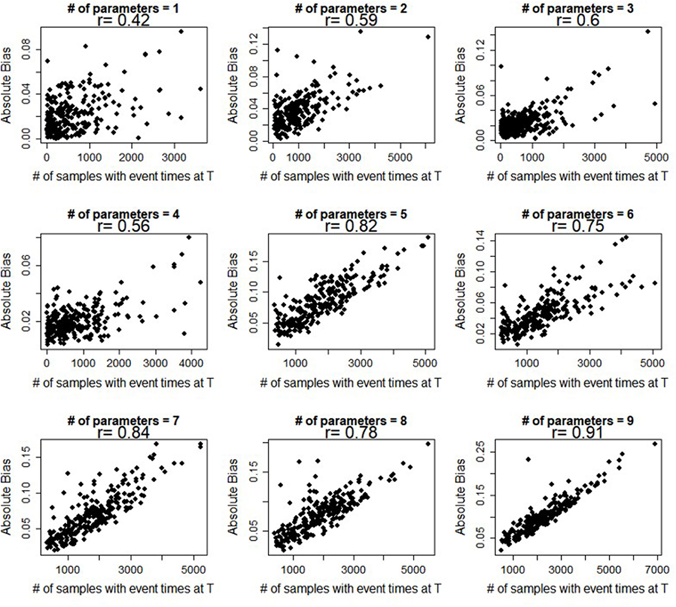
Figure 2. Pearson correlation coefficients. Displays the Pearson correlation coefficient (R) between the number of individuals at the maximum event time and the average absolute bias while increasing the number of parameters holding the censoring rate at 0.5.

FIGURE 3

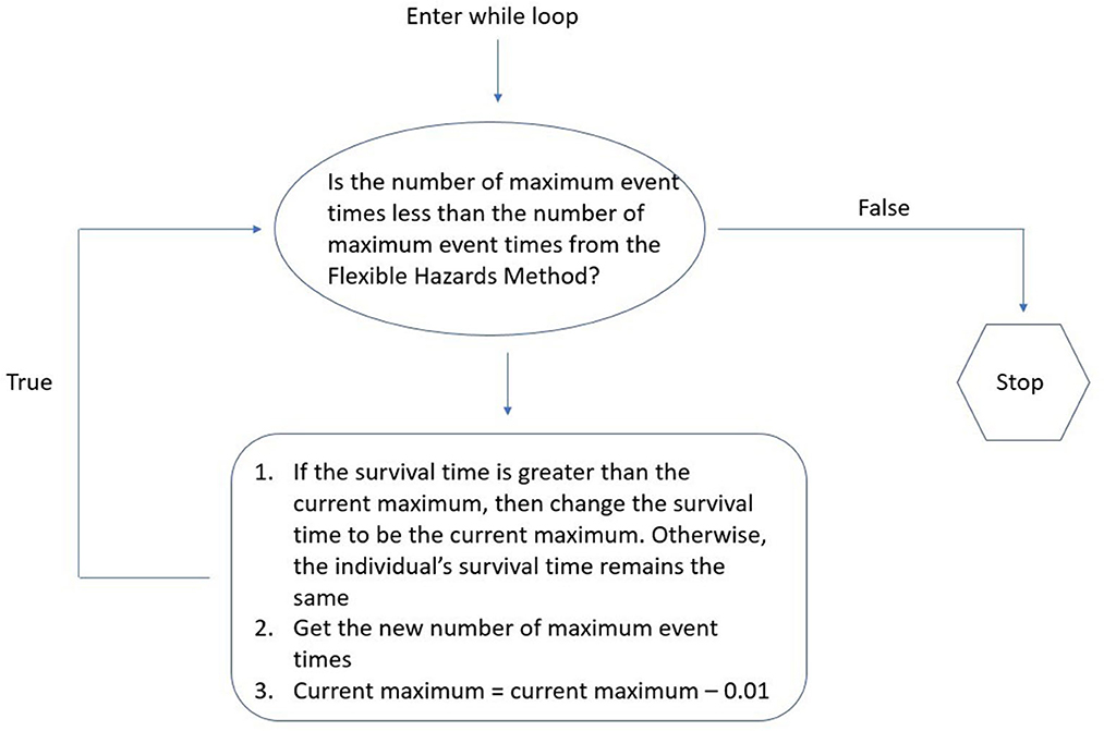
Figure 3. While loop methodology. This figure depicts the while loop methodology for coercing the exponential and Weibull distributions to have the same number of maximum event times as the Flexible Hazards Method.

Moreover, when the exponential and Weibull distributions are forced to have the same proportion of tied maximum event times, at large T (T = 1,000, for example), the Flexible Hazards Method performs almost equivalently to the exponential and Weibull distributions regardless of the number of covariates. Table 4 shows the results of the mean absolute bias for the exponential, Weibull, and Flexible Hazards Method while increasing the number of covariates and increasing the maximum survival time, T, for the Flexible Hazards Method, when the exponential and Weibull distributions have the same proportion of samples at the maximum survival time as the Flexible Hazards Method. At T = 1,000, p = 10, and n = 10,000, the average absolute bias for the Flexible Hazards Method has an interquartile range of (0.035, 0.078) and an average of 0.054. The exponential and Weibull distributions have an interquartile range of approximately (0.029, 0.071) with an average of 0.046. Table 5 shows the results of the average coverage for the exponential, Weibull, and Flexible Hazards Method when increasing both the number of parameters and the maximum event time in the Flexible Hazards Method. At T = 1,000 and p = 10 the average coverage for the Flexible Hazards Method is 0.467 where the average coverage is 0.523 for the exponential distribution and 0.533 for the Weibull distribution. This table shows that the average coverage increases as one increases the maximum event time, T, and while holding the number of parameters constant. It also shows that as we increase the number of covariates, the average coverage decreases across all three approaches. The reader is referred to Supplementary Table 1 for the results of the average absolute bias and Supplementary Table 2 for the results of the average coverage when the sample size was lowered to n = 1,000. Additionally, Supplementary Table 3 gives the median and interquartile range for the proportion of individuals that were drawn to have the maximum event time in the Flexible Hazards Method and the subsequent median and interquartile ranges after the exponential and Weibull distributions were coerced to have similar proportions as that of the Flexible Hazards Method.

TABLE 4

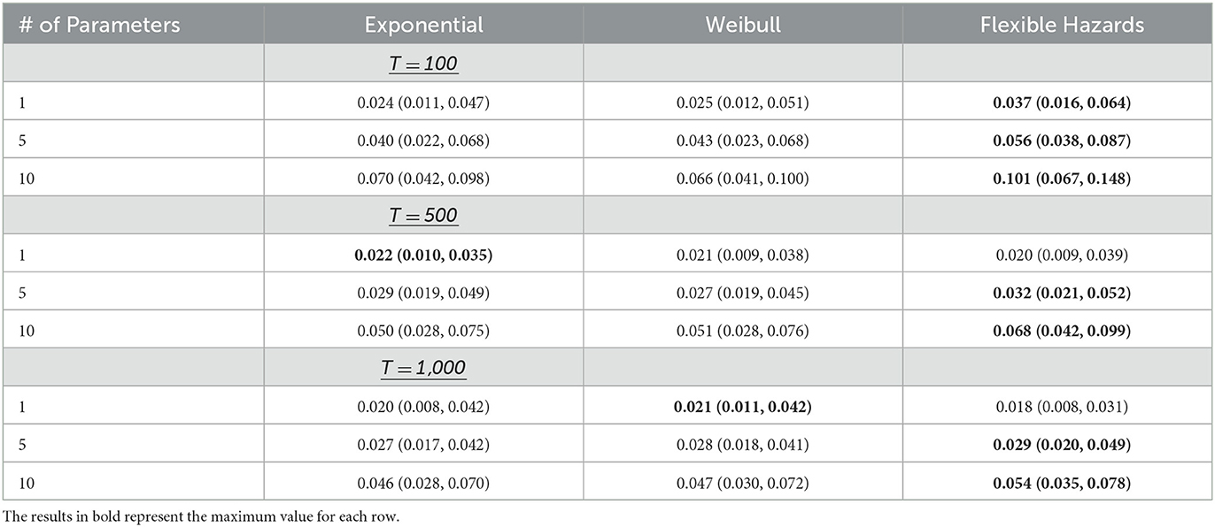
Table 4. The median (IQR) absolute bias in the parameter estimates for the exponential, Weibull, and Flexible Hazards Method across all simulated maximum event times for the Flexible Hazards Method when the number of event times is coerced to be the same across all baseline hazard assumptions.

TABLE 5

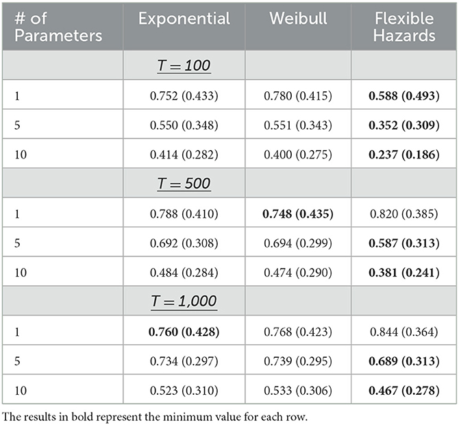
Table 5. The average coverage (standard deviation) in the parameter estimates for the exponential, Weibull, and Flexible Hazards Method across all simulated maximum event times for the Flexible Hazards Method when the number of event times is coerced to be the same across all baseline hazard assumptions.

4. Discussion

The Flexible Hazards Method allows one to simulate time-to-event data from a non-parametric baseline hazard under the CPH model framework. This user-friendly method can be implemented in the coxed R package and has the capacity to handle many different scenarios. However, when simulating time-to-event data using the Flexible Hazards Method, we observed that as the number of covariates in the CPH model was increased, so too does the bias in the estimates of the parameters obtained from fitting the CPH model to the generated data. In the present study, we observed comparable performance between the Flexible Hazards Method and the parametric baseline hazards models in terms of coverage and average absolute bias with large T when there is only a single covariate. Thus, when considering a CPH survival model where only a single covariate is associated with the risk of the event, the Flexible Hazards Method may be preferred as researchers do not have to specify the baseline hazard distribution. However, when the number of risk-associated covariates is increased, we observed a substantial decline in the performance of the Flexible Hazards Method when compared to the exponential and Weibull parametric baseline hazard models. One plausible explanation for this is that when the number of parameters is increased, the number of individuals having event times at the maximum value of T increases. Indeed, when we forced the exponential and Weibull distributions to have the same number of individuals at the maximum event time, the performance of the exponential and Weibull baseline hazards resembled the performance of the Flexible Hazards Method. Graphically, we show how increasing the number of parameters is linked to an increase in the number of individuals with event times exactly equal to the minimum or maximum event time. As we can see from Figure 4, when we have a large negative sum of the individual's covariate effects by parameter coefficients, the received individual survival plot is that of a mirrored “L”. Thus, when generating the individual survival time and taking a random value from a Uniform(0,1) distribution, nearly any resulting value will give us a maximum survival time. The opposite is true when we have a large positive value for X_iβ, the resulting value will almost always be at the minimum survival time. It is recommended when using the Flexible Hazards Method that researchers keep in mind the number of parameters that are to be included in the model as well as the value of the linear predictors. These values must be consciously kept small to prevent the occurrence of clusters of individuals with tied event times at the minimum or maximum times. Using a large value of T will greatly improve the accuracy of the results as was shown that as we increase the value of T, the Flexible Hazards Method performs better. Nevertheless, bias still remains even with increasing T and additional computational burden occurs.

FIGURE 4

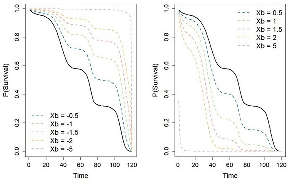
Figure 4. Probability of survival as a function of time. Displays how the absolute increase in the sum of the multiplication between an individual's covariate effects and their corresponding covariate coefficients results in an individual survival plot that is either an “L” shape or the mirror of “L,” thus depicting how we get numerous survival times at either the minimum or maximum value of T.

One potential drawback of our simulation study is not further increasing T to say, 10,000, to see how even larger values of T affect the performance of the Flexible Hazards Method. However, increasing T comes with considerable computational cost, as previously mentioned. The average time for one MC was 1.21 seconds when T = 100; whereas, the average time when T = 1,000 was 7.10 seconds. This made increasing T impractical as the computational cost was too high when conducting MC iterations for the purposes of our simulation studies. Another limitation is that our study only included the exponential and Weibull distributions to benchmark the performance of the Flexible Hazards Method. A case could be made that different distributions should be considered such as a log-normal or a Gompertz baseline hazard; however, as with simulation studies, a general limitation is that not every single combination of parameter values can be evaluated. We provide results here for many different combinations that was able to bring forth many themes in these data. In conclusion, we found that the Flexible Hazards Method presented by Harden and Kropko is a very easy-to-implement method and has a wide array of uses. Caution from the user is needed when more than one parameter is supplied as results can become biased and misleading very quickly. It is recommended to keep the number of linear predictors small and the value of T large.

Future research may include extending the Flexible Hazards Method to facilitate data generation from other time-to-event models, such as the cure rate model. One may also consider creating an easy-to-use built-in R function for simulation-based power and sample size calculations for the Flexible Hazards Method.

Data availability statement

The original contributions presented in the study are included in the article/Supplementary material, further inquiries can be directed to the corresponding author.

Author contributions

JD: Conceptualization, Methodology, Writing—original draft, Writing—review & editing, Formal analysis, Investigation, Visualization. DK: Conceptualization, Methodology, Writing—original draft, Writing—review & editing, Funding acquisition, Project administration, Resources, Supervision.

Funding

The author(s) declare financial support was received for the research, authorship, and/or publication of this article. Research reported was supported by: the Kansas IDeA Network of Biomedical Research Excellence Bioinformatics Core, supported by the National Institute of General Medical Science award P20 GM103418 and the Kansas Institute for Precision Medicine COBRE, supported by the National Institute of General Medical Science award P20 GM130423.

Acknowledgments

We would like to extend our gratitude to: Samuel Boyd, Whitney Shae, Jonah Amponsah, Emily Nissen, Alexander Alsup, Shelby Bell-Glenn, Dr. Jeffrey Thompson, Dr. Nanda Yellapu, and Dr. Dong Pei, for their constructive feedback on this manuscript.

Conflict of interest

The authors declare that the research was conducted in the absence of any commercial or financial relationships that could be construed as a potential conflict of interest.

Publisher's note

All claims expressed in this article are solely those of the authors and do not necessarily represent those of their affiliated organizations, or those of the publisher, the editors and the reviewers. Any product that may be evaluated in this article, or claim that may be made by its manufacturer, is not guaranteed or endorsed by the publisher.

Supplementary material

The Supplementary Material for this article can be found online at: https://www.frontiersin.org/articles/10.3389/fams.2023.1272334/full#supplementary-material

References

1. Kyle R. Long term survival in multiple myeloma. New Eng J Medicine. (1997) 308:314–6. doi: 10.1056/NEJM198302103080604

CrossRef Full Text | Google Scholar

2. Le-Rademacher JG, Peterson RA, Therneau TM, Sanford BL, Stone RM, Mandrekar SJ. Application of multi-state models in cancer clinical trials. Clin Trials. (2018) 15:489–98. doi: 10.1177/1740774518789098

PubMed Abstract | CrossRef Full Text | Google Scholar

3. Clark TG, Bradburn MJ, Love SB, Altman DG. Survival analysis part I: basic concepts and first analyses. Br J Cancer. (2003) 89:232–8. doi: 10.1038/sj.bjc.6601118

PubMed Abstract | CrossRef Full Text | Google Scholar

4. Breslow N. Discussion of the paper by DR Cox. J R Statist Soc B. (1972) 34:216–7.

Google Scholar

5. Therneau T, Grambsch M. Modeling Survival Data: Extending the Cox Model. New York: Springer. (2000). doi: 10.1007/978-1-4757-3294-8

CrossRef Full Text | Google Scholar

6. Cox D. Regression models and life tables (with discussion). J R Stat Soc Series B. (1972) 34:187–220. doi: 10.1111/j.2517-6161.1972.tb00899.x

CrossRef Full Text | Google Scholar

7. Wijk R, Simonsson U. Finding the right hazard function for time-to-event modeling: A tutorial, Shiny application. Parmacomet Syst Pharmacol. (2022) 11:991–1001. doi: 10.1002/psp4.12797

PubMed Abstract | CrossRef Full Text | Google Scholar

8. Lee E, Go O. Survival analysis in public health research. Annu Rev Public Health. (1997) 18:105–34. doi: 10.1146/annurev.publhealth.18.1.105

CrossRef Full Text | Google Scholar

9. Bender R, Augustin T, Blettner M. Generating survival times to simulate Cox proportional hazards models. Stat Med. (2005) 24:1713–23. doi: 10.1002/sim.2059

PubMed Abstract | CrossRef Full Text | Google Scholar

10. Moriña D, Navarro A. The R package survsim for the simulation of simple, complex survival data. J Stat Softw. (2014) 59:1–20. doi: 10.18637/jss.v059.i02

CrossRef Full Text | Google Scholar

11. Jackson C. flexsurv: Flexible parametric survival, multi-state models. (2023). Available online at: http://CRAN.Rproject.org/package=flexsurv (accessed July 21, 2023).

Google Scholar

12. Huang Y, Zhang Y, Zhang Z, Gilbert P. Generating survival times using Cox proportional hazards models with cyclic and piecewise time-varying covariates. Stat Biosci. (2020) 12:324–39. doi: 10.1007/s12561-020-09266-3

PubMed Abstract | CrossRef Full Text | Google Scholar

13. Hendry D. Data generation for the Cox proportional hazards model with time-dependent covariates: a method for medical researches. Stat Med. (2014) 33:436–54. doi: 10.1002/sim.5945

PubMed Abstract | CrossRef Full Text | Google Scholar

14. Montez-Rath ME, Kapphahn K, Mathur MB, Mitani AA, Hendry DJ, Desai M. Guidelines for generating right-censored outcomes from a Cox model extended to accommodate time-varying covariates. J Modern Appl Stat Method. (2017) 16:6. doi: 10.22237/jmasm/1493597100

CrossRef Full Text | Google Scholar

15. Ngwa JS, Cabral HJ, Cheng DM, Gagnon DR, LaValley MP, Cupples LA. Generating survival times with time-varying covariates using the Lambert W function. Commun Stat Simul Comput. (2022) 51:135–53. doi: 10.1080/03610918.2019.1648822

PubMed Abstract | CrossRef Full Text | Google Scholar

16. Zhou M. Understanding the Cox regression models with time-change covariates. Am Stat. (2001) 55:153–5. doi: 10.1198/000313001750358491

CrossRef Full Text | Google Scholar

17. Müller H, Wang J. Hazard rate estimation under random censoring with varying kernels, bandwidths. Biometrics. (1994) 50:61–76. doi: 10.2307/2533197

PubMed Abstract | CrossRef Full Text | Google Scholar

18. Gefeller O, Dette H. Nearest neighbor kernel estimation of the hazard function from censored data. J Stat Comput Simul. (1992) 43:93–101. doi: 10.1080/00949659208811430

CrossRef Full Text | Google Scholar

19. Cai T, Hyndman R, Wand M. Mixed model-based hazard estimation. J Comput Graph Stat. (2002) 11:784–98. doi: 10.1198/106186002862

CrossRef Full Text | Google Scholar

20. Hess K, Serachitopol D, Brown B. Hazard function estimators: a simulation study. Stat Med. (1999) 18:3075–88. doi: 10.1002/(SICI)1097-0258(19991130)18:22<3075::AID-SIM244>3.0.CO;2-6

PubMed Abstract | CrossRef Full Text | Google Scholar

21. Hess K, Gentleman R. muhaz: Hazard function estimation in survival analysis. (2010). Available online at: http://CRAN.R-project.org/package=muhaz (accessed July 21, 2023).

Google Scholar

22. Rebora P, Salim A, Reilly M. bshazard: A flexible tool for nonparametric smoothing of the hazard function. R J. (2014) 6:114–22. doi: 10.32614/RJ-2014-028

CrossRef Full Text | Google Scholar

23. Harden J, Kropko J. Simulating duration data for the cox model. Polit Sci Res Method. (2018) 7:921–8. doi: 10.1017/psrm.2018.19

CrossRef Full Text | Google Scholar

24. Kropko J, Harden J. Coxed: An R package for computing duration-based quantities form the Cox proportional hazards model. R J. (2019) 11:38–45. doi: 10.32614/RJ-2019-042

CrossRef Full Text | Google Scholar

25. Efron B. The efficiency of Cox's likelihood function for censored data. J Am Stat Assoc. (1977) 72:557–65. doi: 10.1080/01621459.1977.10480613

CrossRef Full Text | Google Scholar

26. Therneau TM. A Package for Survival Analysis in R. (2023). Available online at: https://CRAN.R-project.org/package=survival (accessed July 21, 2023).

Google Scholar