Image segmentation using active contours with image structure adaptive gradient vector flow external force

Introduction: Gradient vector flow (GVF) has been proven as an effective external force for active contours. However, its smoothness constraint does not take the image structure into account, such that the GVF diffusion is isotropic and cannot preserve weak edges well.

Methods: In this article, an image structure adaptive gradient vector flow (ISAGVF) external force is proposed for active contours. In the proposed ISAGVF model, the smoothness constraint is first reformulated in matrix form, and then the image structure tensor is incorporated. As the structure tensor characterizes the image structure well, the proposed ISAGVF model can be adaptive to image structure, and the ISAGVF snake performs well on weak edge preservation and deep concavity convergence while possessing some other desirable properties of the GVF snake, such as enlarged capture range and insensitivity to initialization.

Results: Experiments on synthetic and real images manifest these properties of the ISAGVF snake.

1. Introduction

Snakes or active contours are dynamic curves defined within an image domain that can move under the influence of internal and external forces [1]. Usually, the internal force comes from the geometrical properties of the contours and the external force is computed from the image data so that the snake will conform to an object boundary or other desired features within an image. The active contour model has been one of the most successful methods for region of interest (ROI) segmentation, and it can be grouped into two categories: parametric active contours [1] and geometric active contours [2–12]. Although deep learning-based methods launch an upsurge of image segmentation at present [13–17], the active contours are still an active topic (e.g., [18–29]), and we also focus on parametric active contours in this study.

As the external force plays a leading role in the evolution of active contours, and that of the traditional snake model is derived as the gradient vector of the edge map, the traditional snakes suffer from initialization sensitivity and concavity convergence. To this end, several useful external forces have been proposed, such as the balloon forces [30, 31]. However, both issues were not solved satisfactorily until the emergence of the gradient vector flow (GVF) [32]. The GVF snake has an enlarged capture range and can move into the concave boundary. Since the effectiveness of the GVF model became apparent, it became the focus of many studies and there have been many improved variants, e.g., the GGVF [33], CN-GGVF [34], harmonic gradient vector flow (HGVF) [35], GVF based on the minimal surface [36] and adaptive diffusion flow (ADF) based on the harmonic surface [37], motion gradient vector flow (MGVF) [38], ILGVF [39], NBGVF [40], gradient vector convolution (GVC) [41], VEF [42], BVF [43], normal gradient vector flow (NGVF) [44], dynamic directional gradient vector flow (DDGVF) [45], EPGVF [46], GVFOM [47], and GVF based on augmented Lagrangian [48]. Additionally, there are some other interesting applications of the gradient vector flow (e.g., [49–52]). Very recently, Makhanov, etc., proposed some interesting studies on the initialization of the GVF snake [53–56] and Jaouen et al. [57] proposed a vector field for image enhancement, which resembles the GVF field.

Although the GVF model has been proven to be effective and widely employed in image segmentation, the smoothness constraint in GVF does not take into account the image structure and suffers from weak edge leakage and a failure to converge to long and thin indentations. In this study, a novel model called image structure adaptive gradient vector flow (ISAGVF) is proposed. In the ISAGVF model, the smoothness constraint in the GVF model is first reformulated into matrix form, and then the image structure tensor is incorporated into the matrix form energy so that the final diffusion equations for the ISAGVF exhibit an anisotropic diffusion behavior. As a result, the ISAGVF snake can preserve weak edges very well and converge to long and thin indentations. The basic idea of the ISAGVF model has been reported as an abstract in [58].

The remainder of this paper is organized as follows. In the Section 2, the GVF snake is briefly reviewed, and then the proposed ISAGVF algorithm is described in detail in the Section 3. In Section 4, a large number of examples and comparison results are reported to confirm the effectiveness of our model, and the conclusion is drawn in the final section.

2. Background: the snake model and gradient vector flow

Kass et al. defined the active contour model [1] as an elastic curve c(s) = [x(s), y(s)], s ∈ [0, 1], that moves through the spatial domain of an image by minimizing the following energy functional:

$\begin{array}{ll}{E}_{Snake}={\displaystyle {\int }_0^1}\left[\frac{1}{2}(\alpha |c^{\prime }(s){|}^2+\beta |c^{″}(s){|}^2)+\nabla E_{ext}(c)\right]ds,& (1)\end{array}$

where c′(s) and c″(s) denote the first and second derivative of c(s) with respect to the arc s, respectively, α and β are weighting parameters that control the continuity and smoothness of the contour, respectively. The external energy E_ext comes from the image data, such as boundaries. The typical external force for an image I is $\nabla E_{ext}=-\nabla |\nabla I{|}^2$. A snake that minimizes E_snake must satisfy the following Euler-Lagrange equation:

$\begin{array}{ll}\alpha c^{″}(s)-\beta c^{\prime \prime \prime \prime }(s)-\nabla E_{ext}=0.& (2)\end{array}$

Xu and Prince suggested taking the above equation as a force balance equation of internal force and external force, as follows,

$\begin{array}{ll}{F}_{int}+F_{ext}=0,& (3)\end{array}$

where $F_{int}=\alpha c^{″}(s)-\beta c^{\prime \prime \prime \prime }(s)$ and F_ext = −∇E_ext. As F_ext comes from the gradient of the edge map |∇I|², it is non-zero only near edges; as a result, the traditional snake is sensitive to initialization and a failure to converge to concavity. To overcome these shortcomings, Xu and Prince suggest replacing F_ext with a more general one by proposing the gradient vector flow (GVF) [32], which is obtained by minimizing the following energy:

$\begin{array}{l}{E}_{GVF}=\iint \mu ({u_x}^2+{u_y}^2+{v_x}^2+{v_y}^2)\\ +|\nabla f{|}^2|v-\nabla f{|}^{2}dxdy,& (4)\end{array}$

where v(x, y) = [u(x, y), v(x, y)] is the GVF vector, f is the edge map of an image, i.e., f = ∇G_σ*I, and μ is a regularization parameter. It can be observed that when f is large at edge points, the second term dominates the energy in (4) and the GVF vector v(x, y) approximately equals ∇f, while f is small or even zero far away from edges; the first term in (4) is dominant and the GVF vector v(x,y) varies smoothly, and as a result, the GVF snake has a large capture range and can converge to concavity. To minimize the E_GVF, it is converted to solve the following Euler–Lagrange equations:

$\begin{array}{ll}\{\begin{array}{c}\frac{\partial u}{\partial t}=\mu {\nabla }^{2}u-{\left|\nabla f\right|}^2\left(u-f_x\right)\\ \frac{\partial v}{\partial t}=\mu {\nabla }^{2}v-{\left|\nabla f\right|}^2\left(v-f_y\right)\end{array},& (5)\end{array}$

where ∇² is the Laplacian operator. The generalized GVF (GGVF) model is obtained by replacing the constant parameter μ with a spatially varying weighting function g(∇f) = exp(–|∇f|²/k²), and |∇f|² in (5) is replaced b y h(∇f)=1–g(∇f)[33]. The GGVF snake possesses improved convergence to long and thin indentations.

3. ISAGVF: image structure adaptive gradient vector flow

3.1. Proposed ISAGVF model

For the GVF model, we observe the following fact:

$\begin{array}{l}{u_x}^2+{u_y}^2=(u_x{u}_y)\left(\frac{u_x}{u_y}\right)=(u_x{u}_y)\left(\begin{array}{c}10\\ 01\\ \end{array}\right)\left(\frac{u_x}{u_y}\right)\\ ={(\nabla u)}^T\left(\begin{array}{c}10\\ 01\end{array}\right)\nabla u.& (6)\end{array}$

Based on this observation, we reformulate the energy function in (4) in the following matrix form:

$\begin{array}{l}{E}_{GVF}=\iint \mu \left[{(\nabla u)}^{T}W\nabla u+{(\nabla v)}^{T}W\nabla v\right]\\ +|\nabla f{|}^2|v-\nabla f{|}^{2}dxdy,& (7)\end{array}$

where W is the identity matrix $\left(\begin{array}{c}10\\ 01\end{array}\right)$. It is obvious that this identity matrix induces scalar L²-norm and the smoothness constraint in (4) fails to consider the image structure, and finally leads to isotropic diffusion equation (5). Based on this fact, we consider replacing W with a matrix D related to the image structure so that the GVF vectors can diffuse according to the image structure adaptively. The new model is named as image structure adaptive gradient vector flow (ISAGVF) and is formulated as follows:

$\begin{array}{l}{E}_{ISGVF}={\displaystyle \iint \mu \left[{(\nabla u)}^{T}D\nabla u+{(\nabla v)}^{T}D\nabla v\right]}\\ +{\left|\nabla f\right|}^2{\left|v-\nabla f\right|}^{2}dxdy,& (8)\end{array}$

where $D=\left(\begin{array}{c}ab\\ bc\end{array}\right)$ is a symmetric and positive semidefinite matrix. The Euler-Lagrange equations for the ISAGVF energy in (8) are as follows:

$\begin{array}{ll}\{\begin{array}{c}\text{μ }div\left(D\nabla u\right)-{\left|\nabla f\right|}^2\left(u-f_x\right)=0\\ \text{μ }div\left(D\nabla v\right)-{\left|\nabla f\right|}^2\left(v-f_y\right)=0\end{array},& (9)\end{array}$

where div is the divergence operator. A good choice for D is the image structure tensor. For image I, the image structure reads:

$\begin{array}{ll}S\left(\nabla I\right)=\nabla I{(\nabla I)}^T\left(\begin{array}{cc}{I}_x^2& I_x{I}_y\\ I_x{I}_y& I_y^2\end{array}\right).& (10)\end{array}$

S is a symmetric and positive semidefinite matrix. To note, when the image structure S is chosen for D, Equation (9) happens to be the structure tensor-based diffusion in [59], and we will borrow the strategies there to construct the diffusion tensor D from image structure tensor S. A previous study [21] adopted the Hessian matrix, but the Hessian matrix is sensitive to noise due to the second order derivatives.

3.2. Construction of the diffusion matrix d

In this subsection, we will build the matrix D from matrix S. Suppose the eigenvectors of S are $\overrightarrow{v_1}$ and $\overrightarrow{v_2}$, the corresponding eigenvalues are λ₁ and λ₂, $U=(\overrightarrow{v_1},\overrightarrow{v_2})$, and Λ = diag(λ₁, λ₂), the structure tensor S can be decomposed by the principal axis transformation [59], as follows:

$\begin{array}{ll}S(\nabla I)=U^T\Lambda U.& (11)\end{array}$

For convenience, the structure tensor S is rewritten as follows,

$\begin{array}{ll}S=\left(\begin{array}{c}{s}_{11}{s}_{12}\\ s_{12}{s}_{22}\end{array}\right).& (12)\end{array}$

Assume that the matrix S in (12) has an eigenvalue λ and the corresponding eigenvector $\vec{v}={({\psi }_1,{\psi }_2)}^T$. According to the linear algebra, we have the following equations:

$\begin{array}{ll}\left(\begin{array}{c}{s}_{11}{s}_{12}\\ s_{12}{s}_{22}\end{array}\right)\left(\begin{array}{c}{\psi }_1\\ {\psi }_2\end{array}\right)=\lambda \left(\begin{array}{c}{\psi }_1\\ {\psi }_2\end{array}\right),& (13)\end{array}$

which is equivalent to:

$\begin{array}{ll}\left(\begin{array}{l}{s}_{11}-\lambda s_{12}\\ s_{12}{s}_{22}-\lambda \end{array}\right)\left(\begin{array}{c}{\psi }_1\\ {\psi }_2\end{array}\right)=0.& (14)\end{array}$

The eigenvalues of the matrix S in (12) can be determined by the determinant of the left-hand 2 × 2 matrix in (14), which is:

$\begin{array}{ll}{\lambda }_{1,2}=\frac{1}{2}\left[s_{11}+s_{22}\pm \sqrt{{(s_{11}-s_{22})}^2+4s_{12}^2}\right],& (15)\end{array}$

where λ₁ corresponds to the “+” sign in (15). The corresponding eigenvectors $\overrightarrow{v_1}={({\phi }_1,{\phi }_2)}^T$ and $\overrightarrow{v_2}={({\zeta }_1{\zeta }_2)}^T$take the following forms:

$\begin{array}{ll}\{\begin{array}{c}{\phi }_1=\frac{2s_{12}}{\sqrt{{(s_{22}-s_{11}+\sqrt{{\left(s_{11}-s_{22}\right)}^2+4s_{12}{}^2})}^2+4s_{12}{}^2}}\\ {\phi }_2=\frac{s_{22}-s_{11}+\sqrt{{\left(s_{11}-s_{22}\right)}^2+4s_{12}{}^2}}{\sqrt{{(s_{22}-s_{11}+\sqrt{{\left(s_{11}-s_{22}\right)}^2+4s_{12}{}^2})}^2+4s_{12}{}^2}}\end{array},& (16)\end{array}$

$\begin{array}{ll}\{\begin{array}{c}{\zeta }_1=\frac{2s_{12}}{\sqrt{{(s_{22}-s_{11}-\sqrt{{\left(s_{11}-s_{22}\right)}^2+4s_{12}{}^2})}^2+4s_{12}{}^2}}\\ {\zeta }_2=\frac{s_{22}-s_{11}+\sqrt{{\left(s_{11}-s_{22}\right)}^2+4s_{12}{}^2}}{\sqrt{{(s_{22}-s_{11}-\sqrt{{\left(s_{11}-s_{22}\right)}^2+4s_{12}{}^2})}^2+4s_{12}{}^2}}\end{array},& (17)\end{array}$

Since S has the form in (10), following the discussion above, we can get the following results:

$\begin{array}{ll}\{\begin{array}{c}{\lambda }_1={\left|\nabla I\right|}^2\\ \overrightarrow{v_1}={\left(I_x/\left|\nabla I\right|,I_y\left|\nabla I\right|\right)}^T\end{array},& (18)\end{array}$

$\begin{array}{ll}\{\begin{array}{c}{\lambda }_2=0\\ \overrightarrow{v_2}={\left(-I_y/\left|\nabla I\right|,I_x/\left|\nabla I\right|\right)}^T\end{array}& (19)\end{array}$

It is easy to verify that the eigenvector $\overrightarrow{v_1}$ is parallel to the gradient vector, whereas $\overrightarrow{v_2}$ is orthogonal. The eigenvalues λ₁ and λ₂ can be used as descriptors of local structure [59]; for instance, constant areas are characterized by λ₁ = λ₂ = 0 and straight edges give λ₁≫λ₂ = 0.

However, the image structure tensor S cannot be directly employed for D as λ₂ = 0 means that the vectors diffuse always merely along the gradient directions, therefore destroying the edges. To construct the reasonable diffusion tensor D, we choose the orthonormal eigenvectors of S, i.e., $\overrightarrow{v_1}$ and $\overrightarrow{v_2}$, as the eigenvectors of D, while the eigenvalues of D denoted by ω₁ and ω₂ are different from those of S, which depends on the goal of application [59]. Then, D can be constructed as:

$\begin{array}{ll}D={\left({\overrightarrow{v}}_1{\overrightarrow{v}}_2\right)}^T\left(\begin{array}{cc}{\omega }_1& 0\\ 0& {\omega }_2\end{array}\right)\left({\overrightarrow{v}}_1{\overrightarrow{v}}_2\right).& (20)\end{array}$

Using (16) and (17), D is finally represented as:

$\begin{array}{l}D=\\ \left(\begin{array}{cc}\frac{1}{2}({\omega }_1+{\omega }_2+\frac{\left({\omega }_2-{\omega }_1\right)\left(s_{22}-s_{11}\right)}{\sqrt{{\left(s_{11}-s_{22}\right)}^2+4s_{12}{}^2}})& \frac{({\omega }_1-{\omega }_2)s_{12}}{\sqrt{{(s_{11}-s_{22})}^2+4s_{12}{}^2}}\\ \frac{({\omega }_1-{\omega }_2)s_{12}}{\sqrt{{(s_{11}-s_{22})}^2+4s_{12}{}^2}}& \frac{1}{2}({\omega }_1+{\omega }_2-\frac{\left({\omega }_2-{\omega }_1\right)\left(s_{22}-s_{11}\right)}{\sqrt{{\left(s_{11}-s_{22}\right)}^2+4s_{12}{}^2}})\end{array}\right).\end{array}(21)$

The performances of the proposed ISAGVF model mostly depend on the choice of the eigenvalues ω₁ and ω₂. ω₁ represents the diffusion coefficient parallel to the gradient vector, while ω₂ is the diffusion coefficient along the edges. The choice of ω₁ and ω₂ conforms to the following criterion [59]: a higher value implies that the diffusion in the direction of the corresponding eigenvector will be encouraged. In the proposed model, ω₁ and ω₂ take the following form for the application on hand:

$\begin{array}{ll}\{\begin{array}{c}{\omega }_1=\frac{1}{1+{\left(\frac{\left|\nabla I\right|}{K}\right)}^2}\\ {\omega }_2=1\end{array},& (22)\end{array}$

where K is the gradient threshold of a given image. The settings of parameter K will be further elucidated in Section 4. It can be observed that

(1) For |∇I| → ∞, i.e., the edges, ${\omega }_1(|\nabla I|)/{\omega }_2(|\nabla I|)=1/(1+{(|\nabla I|/K)}^2)\to 0$, ISAGVF prefers diffusing along the edge. As a result, the edge can be preserved, and the noise can be removed;

(2) For |∇I| → 0, i.e., the homogeneous region, ω₁(|∇I|) = ω₂(|∇I|) = 1 > 0, diffusing is isotropic, and the noise can be reduced accordingly.

In this way, the proposed ISAGVF diffuses adaptively according to the image structure, which would help the snake to preserve weak edges and enter narrow and deep concavities and even complex structures. The details of numerical implementation have been described by [59].

4. Experimental results and discussion

In this section, we evaluate the performance of the ISAGVF snake in terms of capture range, weak edge preservation, and narrow and deep concavity convergence, as well as complex structure convergence, and make comparisons with several popular GVF-like models, including the GVF [32], GGVF [33], NGVF [44], ILGVF [39], VEF [42], and BVF [43]. The parameters for all snakes in our experiments are α = 0.1, β = 0.1, and time step τ = 0.5, and the image intensity is normalized to range [0, 1]. For an image of size M · N, the iteration for the calculation of all GVF-like models is $\sqrt{M·N}$, and the time step is 1 [<1/(4μ)]. To obtain a large capture range and more regular force field, the parameter μ for GVF, NGVF, ILGVF is 0.2, and 0.1 for the ISAGVF, and K = 0.5 for GGVF, ω = 1.0 for BVF, and the convolution kernel size for the VEF model is a quarter of the image size. Parameter K for the ISAGVF is a constant that determines the contrast of the edges to be preserved and it is 0.1, unless otherwise stated [59]. As different models adopt different mechanisms, the same parameter may not be optimal for different models; as a result, we adopted different values for some parameters in different models so that the performances of different models are optimal.

4.1. Common properties: enlarged capture range and initialization insensitivity

To confirm that the proposed model has a sufficient capture range, the usually employed room and U-shape images are enlarged to a size of 128 × 128 pixels, while the size of both objects is fixed. The enlarged images are shown in Figure 1A, the corresponding ISAGVF fields are shown in Figure 1B, and the initial contours and the evolution results of the proposed ISAGVF snake model for three different objects are shown in Figures 1C–E, respectively. Although the initializations are placed far away, across or inside the objects, the ISAGVF snakes converge to the true boundaries regularly; this fact manifests that the proposed ISAGVF snake is insensitive to initialization and has a large capture range.

FIGURE 1

Figure 1. Capture range enlargement and initialization insensitivity of the ISAGVF snake. (A) Test images. (B) ISAGVF fields. (C–E) Different initializations and evolutions of the ISAGVF snakes.

4.2. Narrow and deep concavity convergence

It is well-known that the GVF snake can converge to U-shape concavity, but when the concavity becomes narrower and deeper, it is very difficult for the GVF snake to converge. However, the proposed ISAGVF snake possesses great power for this issue as the ISAGVF model takes into account the image structure. Figure 2 shows three testing concavity images. The first one is an “E”-shaped image with an upper concavity width of 3 pixels and a depth of 35 pixels and the bottom one has a width of 3 pixels and a depth of 40 pixels. One can see that the BVF snake and the proposed ISAGVF snake dived into both concavities successfully, but the others failed. Another interesting observation is that the GGVF snake succeeded in a concavity with a depth of 35 pixels but failed in the concavity with a depth of 40 pixels; the reason behind this fact is that the GGVF model is just a weighted version of the GVF model (both are isotropic). The second one is a “T”-shaped image with a horizontal concavity with a width of 5 pixels and length of 40 pixels, and a vertical concavity with a width of 3 pixels and depth of 40 pixels. It was observed that the GGVF, NGVF, BVF, and ISAGVF snakes converged to the horizontal concavity, whereas just the ISAGVF snake succeeded in the vertical one, although the vertical concavity is narrower. For the cross image in the third row, the four concavities each have a width of 3 pixels and depth of 50 pixels. It was observed that just the NGVF and ISAGVF snakes dived into the concavities successfully; the GVF, GGVF, and VEF snakes were halfway from converging in the concavities, while the ILGVF and BVF snakes were merely on the ready line. From these results, the performance of the ISAGVF snake with respect to concavity convergence is verified.

FIGURE 2

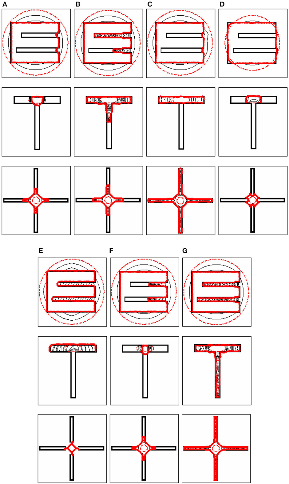
Figure 2. Concavity convergence of the snakes. The first testing image is an “E”-shaped image with an upper concavity width of 3 pixels and depth of 35 pixels and the bottom concavity has a width of 3 pixels and length of 40 pixels. The second image is a “T”-shaped image with a horizontal concavity with a width of 5 pixels and depth of 40 pixels, and a vertical concavity with a width of 3 pixels and depth of 40 pixels. The third one is a cross-shaped image with four concavities each with a width of 3 pixels and depth of 50 pixels. The convergence results of (A) GVF, (B) GGVF, (C) NGVF, (D) ILGVF, (E) BVF, (F) VEF, and (G) ISAGVF snakes are shown as solid red lines.

4.3. Weak edge preserving

A weak edge often appears in images and it is nuisance for image segmentation, especially for snake-based methods when there are some strong edges nearby. Figure 3A shows two examples. The first one is an image of two disks (see the upper panel). The upper-left edge of the outer disk is blurred and weak and the neighboring edge of the inner one is strong. The second example is an image composed of three gray values (0, 255, and 245, see the bottom panel). The edge between the region of gray value 0 and that of gray value 255 is strong, whereas the edge between the region of gray value 255 and that of gray value 245 is weak. Both edge maps are shown in Figure 3B, from which one can see that the weak edges in both examples are almost invisible, and the snake contours are used to being attracted by the strong edges nearby. The convergence results of (C) GVF, (D) GGVF, (E) NGVF, (F) ILGVF, (G) BVF, (H) VEF, and (I) ISAGVF snakes are shown in Figures 3C–I, respectively. As expected, all the models employed for comparison failed to capture the weak edge, while the proposed ISAGVF snake resisted the lure from the strong edge and caught the weak edge successfully. To note, the ILGVF snake expanded the initial contour slightly as the initialization was not in the territory of the force filed, although the initial contour touched the weak edge. By contrast, the proposed ISAGVF snake dealt with this issue gracefully thanks to taking into account the image structure. In these experiments, the parameters were K = 0.01 for the ISAGVF model.

FIGURE 3

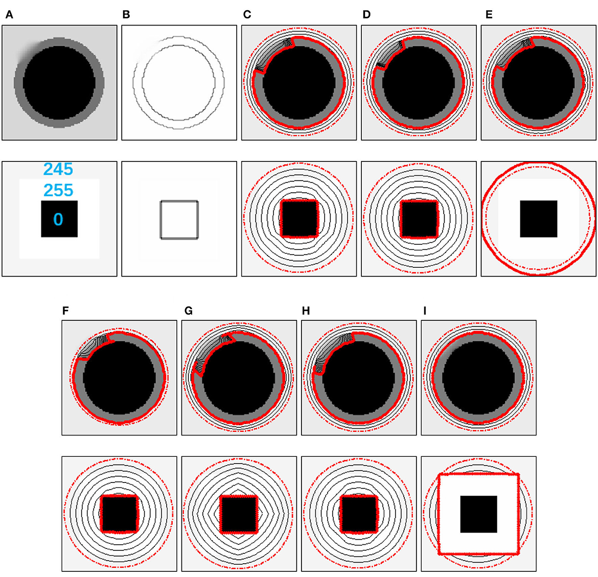
Figure 3. Weak edge preserving demonstrations. There are two weak edge examples. (A) The test images. (B) Edge maps. The convergence results of (C) GVF, (D) GGVF, (E) NGVF, (F) ILGVF, (G) BVF, (H) VEF, and (I) ISAGVF snakes are shown as solid red lines, and the dash-point circles in red are the initial contours.

4.4. Complex structure convergence

It is well-known that the GVF snake can converge to the U-shape concavity; however, when the concavity is complex, it remains a challenge for the GVF-like methods. The reason behind this is that complex structures may make forces computed from their gradient have different directions, thus making the snake contour stop at an unexpected position. In this subsection, we present six examples with various characteristics to illustrate that the proposed ISAGVF snake has a great advantage in this respect as the ISAGVF model takes the image structure into account. Figure 4 shows the results. The first example is the 3-shape, which has two concavities. The GVF, GGVF, and NGVF stopped at the gate of the concavities, and the ILGVF snake tried to enter the concavities but failed, although the initial contour was very close to the object. After a period of wandering, the BVF snake entered the lower concavity but could not do anything for the upper concavity. By contrast, the VEF and ISAGVF snakes successfully dived into the two concavities. For the other five examples in Figure 4, only the ISAGVF snake succeeded in converging to each concavity; all the other models failed at all concavities. The great superiority of the ISAGVF snake in taking the image structure into account can be observed from these examples.

FIGURE 4

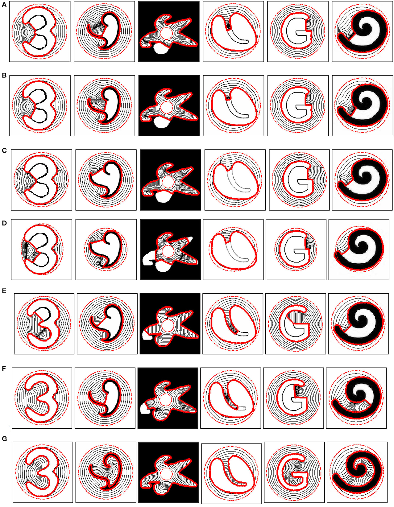
Figure 4. Demonstration and comparison of complex concavity convergence. The convergence results of (A) GVF, (B) GGVF, (C) NGVF, (D) ILGVF, (E) BVF, (F) VEF, and (G) ISAGVF snakes are shown by the solid red lines, and the dash-point circles in red are the initial contours.

4.5. Real images

The proposed ISAGVF snake was also applied to some real images to verify its superiority. In these cases, we had to cope with intensity inhomogeneity, noise, and weak edges neighbored by strong ones. Hence, K was chosen as 0.01 for the proposed ISAGVF. The image in the Figure 5 is an echocardiographic image of the left ventricle, where the snake contour could be harassed by intensity inhomogeneity, noise, and weak edges. The image is smoothed with a Gaussian filter of a standard deviation of 3 before the edge map was derived. One can see that the GVF and VEF snakes leaked out in both upper and lower areas and the other two also converged to an incorrect position. By contrast, the proposed ISAGVF model stuck to the desired edges. Figure 6 presents the results of a vessel with many branches. To derive the edge map, the image is preprocessed with a Gaussian filter with a standard deviation of 1. With the same initialization, only the ISAGVF snake extracted the boundary successfully, while others blocked the way to some branches.

FIGURE 5

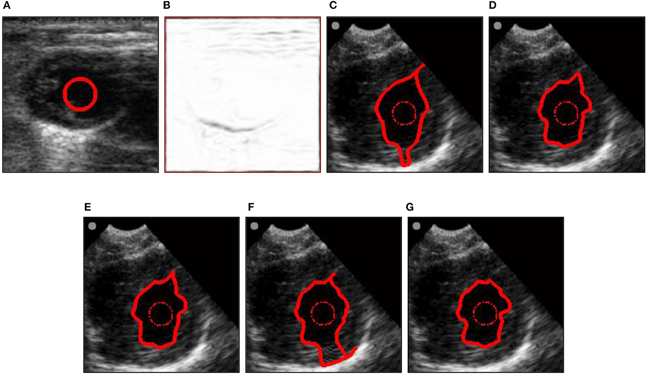
Figure 5. Segmentation of an echocardiographic image. (A) Original image. (B) The edge map. (C–G) The convergence results of the (C) GVF, (D) GGVF, (E) NGVF, (F) VEF, and (G) ISAGVF snakes are shown by the solid red lines, and the dash-point circles in red are the initial contours.

FIGURE 6

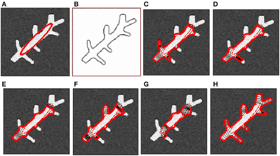
Figure 6. Demonstration of a vessel image. (A) Original image. (B) The edge map. (C–H) The convergence results of the (C) GVF, (D) GGVF, (E) NGVF, (F) BVF, (G) VEF, and (H) ISAGVF snakes are shown by the solid red lines, and the dash-point circles in red are the initial contours.

The image in Figure 7 is a person holding up a stick on a horse. The difficulties of this example reside in the concave region between the person and the stick and the neck and the chin, as well as the tail and the leg of the horse, as pointed out by the three red arrows in Figure 7A. The person with the stick is cropped to show the close-up of the converged result of each method. It can be observed that just the GGVF and ISAGVF snakes can cope with the concavity between the tail and the leg of the horse; the GGVF model takes the image structure into account to some degree as it adopts the edge map as weight, while the ISAGVF model takes the image structure into account in the diffusion process. Just for this reason, only the proposed ISAGVF snake can successfully converge to the other two concave regions. When the close-ups of the converged results of each method are inspected, the GVF snake cannot preserve the head of the person and the thin stick (see Figure 7C), while the GGVF snake can correctly capture the head and the thin stick; however, it failed to converge to the concave region (see Figure 7D). In the case of NGVF, the diffusion continues in the normal direction and the convergence result is irregular (Figure 7E). The result of the BVF snake in Figure 7F shows that it can capture the head of the person correctly but cannot capture the thin stick and cannot enter the concavity. Although the VEF snake can extract the head of the person, it fails to catch the stick (see Figure 7G). In addition, the proposed ISAGVF snake can catch the thin stick and enter the concave region successfully (see Figure 7H). The superiority of the ISAGVF snake by taking the image structure into account is demonstrated thoroughly.

FIGURE 7

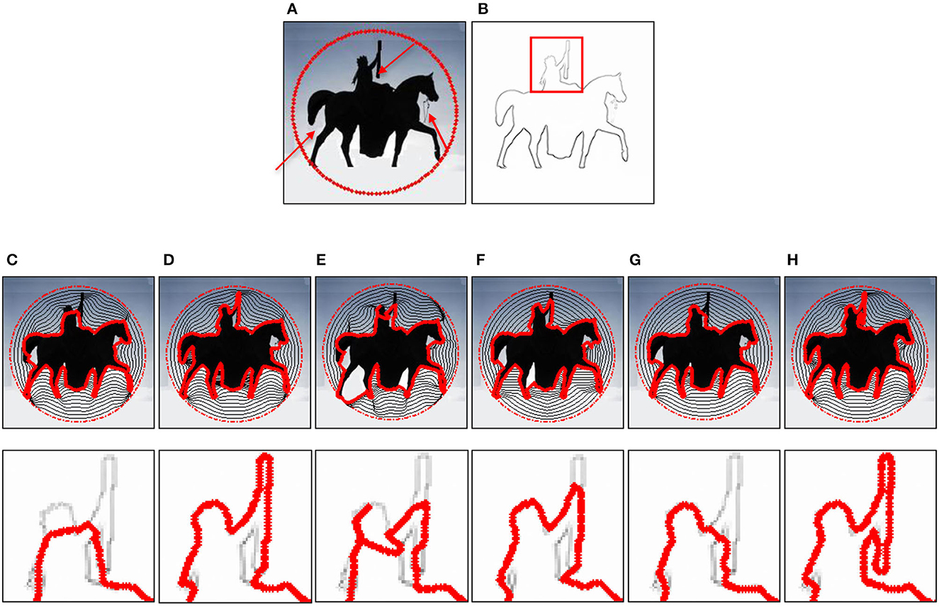
Figure 7. Demonstration of a horse image. (A) Original image. (B) The edge map. (C–H) The convergence results of the (C) GVF, (D) GGVF, (E) NGVF, (F) BVF, (G) VEF, and (H) ISAGVF snakes are shown by the solid red lines, and the dash-point circles in red are the initial contours. The results in the second row in (C–H) are the close-ups of the corresponding results in the first row in the red rectangle in (B).

Figure 8 shows an image of a USB flash disk on the back of a hand. The disk yields a strong edge near the sleeve opening that may probably attract the snake contour. The results show that only the proposed ISAGVF snake can resist the lure of the strong edge and correctly capture the shape of the hand. Figure 9 shows more results of the ISAGVF snake on real images, and the results are satisfactory.

FIGURE 8

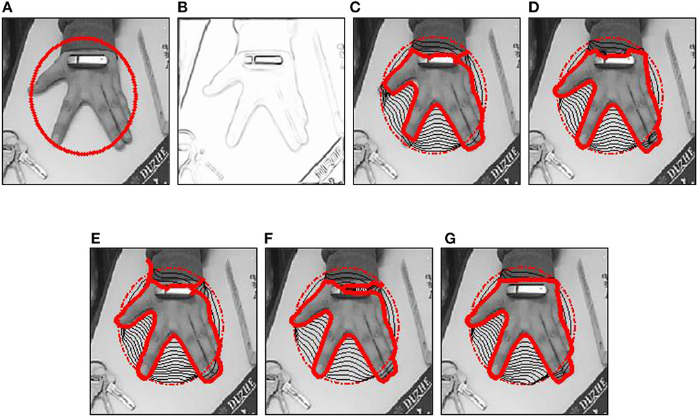
Figure 8. Demonstration on an image of a hand. (A) Original image, (B) The edge map. (C–G) The convergence results of the (C) GVF, (D) GGVF, (E) NGVF, (F) VEF, and (G) ISAGVF snakes are shown by the solid red lines, and the dash-point circles in red are the initial contours. The image in (A) was smoothed using a Gaussian filter with a standard deviation of 1.

FIGURE 9

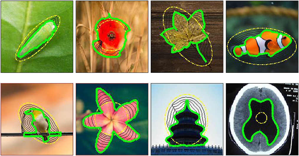
Figure 9. More results of the proposed ISAGVF snake on real images. The dash-point lines in yellow are the initial contours and the solid green lines are the convergence results.

4.6. Discussion

As we know, it is contradictory to preserve weak edges and smooth noise simultaneously for the external force of the snake model. Parameter K in the proposed ISAGVF model serves as the gradient threshold, the value of which depends on the preservation of the magnitude of the gradient of the weak edge. Through a lot of tests, we found that, for the vast majority of the images, K ranges from 0.01 to 0.5. At the same time, a large K can also suppress noise to some degree; if the image has a lot of noise, we can choose a relatively larger K to suppress it without disturbing the edge. As shown in the top row of Figure 10, the snake model stuck in the concavity due to noise with the smallest K. However, as K increases, it resists noise more and becomes better at entering concavities. Additionally, when there are some weak edges in the image, we should make it smaller to preserve the edge of the object. The results in the bottom row of Figure 10 demonstrate our analysis, i.e., a K that is too large will lead to weak boundary leakage. Parameter μ mainly controls the diffusion degree of the external force field in homogeneous region. The larger μ is, the larger the diffusion degree of the external force field. In other words, a large μ helps to smooth noise and results in a large capture range. Therefore, K and μ are closely linked. As we can see from the third row in Figure 10, when μ takes a smaller value, the capture range of the vector field is not enough, and thus the initialization needs to be close to the boundary of the object, but at the same time the weak edge can be protected. As μ increases, the capture range becomes increasingly larger, and finally, the strong edge may attract the weak edge. In short, the parameters K and μ can change interactively to smooth noise, preserve weak edges, and extend the capture range.

FIGURE 10

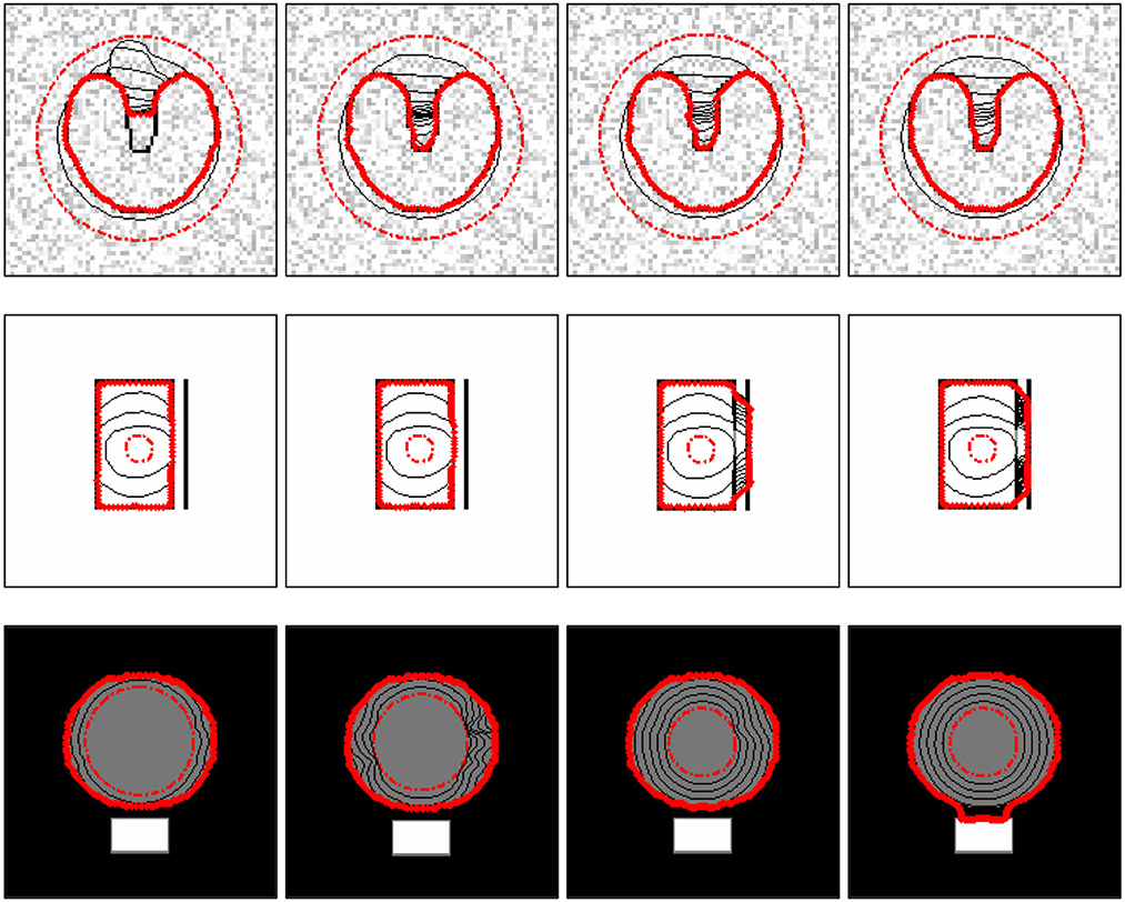
Figure 10. Test of the parameters K and μ. Top row: the segmentation results of images with noise. Second row: the segmentation results of images where there are strong edges nearby weak edges. The μ is 0.2 and K-values from left to right are 0.01, 0.05, 0.1, and 0.5, respectively. For the third row, K is 0.1 and μ values from left to right are 0.001, 0.02, 0.1, and 0.2, respectively.

5. Conclusion

A novel external force called image structure adaptive gradient vector flow (ISAGVF) is proposed for active contours. Given that the smoothness constraint of the GVF model does not take the image structure into account, the smoothness constraint was rewritten in a matrix form and the image structure tensor was introduced into the smoothness constraint, such that the proposed ISAGVF model behaves in an anisotropic manner. A simple and effective method was also adopted to construct the diffusion tensor from the image structure tensor. Experimental results on both synthetic and real images showed that the ISAGVF snake is superior to other popular models in terms of weak edge preservation, deep concavity entering, and some complex image convergence.

Data availability statement

The original contributions presented in the study are included in the article/supplementary material, further inquiries can be directed to the corresponding authors.

Author contributions

DW: Methodology, Software, Writing—original draft. XD: Funding acquisition, Investigation, Resources, Validation, Visualization, Writing—review and editing. WL: Visualization, Data curation, Methodology, Project administration, Writing—original draft. YW: Conceptualization, Funding acquisition, Investigation, Supervision, Writing—review and editing. All authors contributed to the article and approved the submitted version.

Funding

The author(s) declare financial support was received for the research, authorship, and/or publication of this article. This study was supported in part by the National Science Foundation of China (NSFC) (61976241).

Conflict of interest

The authors declare that the research was conducted in the absence of any commercial or financial relationships that could be construed as a potential conflict of interest.

Publisher's note

All claims expressed in this article are solely those of the authors and do not necessarily represent those of their affiliated organizations, or those of the publisher, the editors and the reviewers. Any product that may be evaluated in this article, or claim that may be made by its manufacturer, is not guaranteed or endorsed by the publisher.

References

1. Kass M, Witkin A, Terzopoulos D. Snake: active contour models. Int J Comput Vis. (1988) 1:321–31. doi: 10.1007/BF00133570

CrossRef Full Text | Google Scholar

2. Caselles V, Catte F, Coll T, Dibos F. A geometric model for active contours. Numer Math. (1993) 66:1–31. doi: 10.1007/BF01385685

CrossRef Full Text | Google Scholar

3. Gui L, Li C, Yang X. Medical image segmentation based on level set and isoperimetric constraint. Phys Med. (2017) 42:162–73. doi: 10.1016/j.ejmp.2017.09.123

PubMed Abstract | CrossRef Full Text | Google Scholar

4. Zhao Y, Guo S, Luo M, Shi X, Bilello M, Zhang S, et al. level set method for multiple sclerosis lesion segmentation. Magn Reson Imaging. (2018) 49:94–100. doi: 10.1016/j.mri.2017.03.002

PubMed Abstract | CrossRef Full Text | Google Scholar

5. Khadidos A, Sanchez V, Li C-T. Weighted level set evolution based on local edge features for medical image segmentation. IEEE Transact Image Process. (2017) 26:1979–91. doi: 10.1109/TIP.2017.2666042

PubMed Abstract | CrossRef Full Text | Google Scholar

6. Ali H, Sher A, Saeed M, Rada L. An active contour image segmentation model with de-hazing constraints. IET Image Process. (2020). 14:921–8. doi: 10.1049/iet-ipr.2018.5987

CrossRef Full Text | Google Scholar

7. Liu G, Zou J. Level set evolution with sparsity constraint for object extraction. IET Image Process.(2018) 12:1413–22. doi: 10.1049/iet-ipr.2017.0939

CrossRef Full Text | Google Scholar

8. Karn PK, Biswal B, Samantaray SR. Robust retinal blood vessel segmentation using hybrid active contour model. IET Image Process. (2019) 13:440–50. doi: 10.1049/iet-ipr.2018.5413

PubMed Abstract | CrossRef Full Text | Google Scholar

9. Chen Y, Zhang J, Mishra A, Yang J. Image segmentation and bias correction via an improved level set method. Neurocomputing. (2011) 74:3520–30. doi: 10.1016/j.neucom.2011.06.006

CrossRef Full Text | Google Scholar

10. Wang Y, Wang H, Xu Y. Texture segmentation using vector-valued Chan-Vese model driven by local histogram. Comp Elect Eng. (2013) 39:1506–15. doi: 10.1016/j.compeleceng.2013.03.017

CrossRef Full Text | Google Scholar

11. Wu H, Appia V, Yezzi A. Numerical conditioning problems and solutions for nonparametric IID statistical active contours. IEEE Transact Pattern Anal Mach Intell. (2013) 35:1298–311. doi: 10.1109/TPAMI.2012.207

PubMed Abstract | CrossRef Full Text | Google Scholar

12. Kim W, Kim C. Active contours driven by the salient edge energy model. IEEE Transact Image Process. (2012) 22:1667–73. doi: 10.1109/TIP.2012.2231689

PubMed Abstract | CrossRef Full Text | Google Scholar

13. Wang W, Wang Y, Wu Y, Lin T, Li S, Chen B. Quantification of full left ventricular metrics via deep regression learning with contour-guidance. IEEE Access. (2019) 7:47918–28. doi: 10.1109/ACCESS.2019.2907564

CrossRef Full Text | Google Scholar

14. Shen W, Xu W, Zhang H, Sun Z, Ma J, Ma X, et al. Automatic segmentation of the femur and tibia bones from X-ray images based on pure dilated residual U-Net. Inverse Prob Imaging. (2021) 15:1333–46. doi: 10.3934/ipi.2020057

CrossRef Full Text | Google Scholar

15. Zhao C, Xiang S, Wang Y, Cai Z, Shen J, Zhou S, et al. Context-aware network fusing transformer and V-Net for semi-supervised segmentation of 3D left atrium. Expert Syst Appl. (2023) 214:119105. doi: 10.1016/j.eswa.2022.119105

CrossRef Full Text | Google Scholar

16. Chen LC, Papandreou G, Kokkinos I, Murphy K, Yuille AL. DeepLab: semantic image segmentation with deep convolutional nets, atrous convolution, and fully connected CRFs. IEEE Trans Pattern Anal Mach Intell. (2018) 40:834–48. doi: 10.1109/TPAMI.2017.2699184

PubMed Abstract | CrossRef Full Text | Google Scholar

17. Zhang H, Zhang W, Shen W, Li N, Chen Y, Li S, et al. Automatic segmentation of the left ventricle from MR images based on nested U-Net with dense block. Biomed Signal Process Control. (2021) 68:102684. doi: 10.1016/j.bspc.2021.102684

CrossRef Full Text | Google Scholar

18. Uhlmann V, Fageot J, Unser M. Hermite snakes with control of tangents. IEEE Trans Image Process. (2016) 25:2803–16. doi: 10.1109/TIP.2016.2551363

PubMed Abstract | CrossRef Full Text | Google Scholar

19. Delgado-Gonzalo R, Uhlmann V, Schmitter D, Unser M. Snakes on a plane-A perfect snap for bioimage analysis. IEEE Signal Processing Mag. (2015) 32:41–8. doi: 10.1109/MSP.2014.2344552

CrossRef Full Text | Google Scholar

20. Zareei A, Karimi A. Liver segmentation with new supervised method to create initial curve for active contour. Comput Biol Med. (2016) 75:139–50. doi: 10.1016/j.compbiomed.2016.05.009

PubMed Abstract | CrossRef Full Text | Google Scholar

21. Qian Q, Cheng K, Qian W, Deng Q, Wang Y. Image segmentation using active contours with hessian based gradient vector flow external force. Sensors. (2022) 22:4956. doi: 10.3390/s22134956

PubMed Abstract | CrossRef Full Text | Google Scholar

22. Zhang Z, Duan C, Lin T, Zhou S, Wang Y, Gao X, et al. A novel external force for active contour based image segmentation. Inf Sci. (2020) 506:1–18. doi: 10.1016/j.ins.2019.08.003

CrossRef Full Text | Google Scholar

23. Song TH, Sanchez V, EIDaly H, Rajpoot NM. Dual-channel active contour model for megakaryocytic cell segmentation in bone marrow trephine histology images. IEEE Trans Biomed Eng. (2017) 64:2913–23. doi: 10.1109/TBME.2017.2690863

PubMed Abstract | CrossRef Full Text | Google Scholar

24. Berenguer-Vidal R, Verdú-Monedero R, Morales-Sánchez J, Sellés-Navarro I, Del Amor R, García G, et al. Automatic segmentation of the retinal nerve fiber layer by means of mathematical morphology and deformable models in 2D optical coherence tomography imaging. Sensors. (2021) 21:8027. doi: 10.3390/s21238027

PubMed Abstract | CrossRef Full Text | Google Scholar

25. Maneerat A, Visitsattapongse S, Pintavirooj C. Bone mineral density screening system using CMOS-sensor X-ray detector. Sensors. (2021) 21:7148. doi: 10.3390/s21217148

PubMed Abstract | CrossRef Full Text | Google Scholar

26. Jia D, Zhang C, Wu N, Guo Z, Ge H. Multi-layer segmentation framework for cell nuclei using improved GVF Snake model, Watershed, and ellipse fitting. Biomed Signal Process Control. (2021) 67:102516. doi: 10.1016/j.bspc.2021.102516

CrossRef Full Text | Google Scholar

27. Yu S, Lu Y, Molloy D. A dynamic-shape-prior guided snake model with application in visually tracking dense cell populations. IEEE Transact Image Process. (2019) 28:1513–27. doi: 10.1109/TIP.2018.2878331

PubMed Abstract | CrossRef Full Text | Google Scholar

28. Zhao SH Li G, Zhang W, Gu J. Automatical intima-media border segmentation on ultrasound image sequences using a Kalman filter snake. IEEE Access. (2018) 6:40804–10. doi: 10.1109/ACCESS.2018.2856244

CrossRef Full Text | Google Scholar

29. Manno-Kovacs A. Direction selective contour detection for salient objects. IEEE Transact Circ Syst Video Technol. (2018) 29. doi: 10.1109/TCSVT.2018.2804438

CrossRef Full Text | Google Scholar

30. Cohen LD. On active contour models and balloons. CVGIP Image Understand. (1991) 53:211–8. doi: 10.1016/1049-9660(91)90028-N

CrossRef Full Text | Google Scholar

31. Cohen LD, Cohen I. Finite-element methods for active contour models and balloons for 2-D and 3-D images. IEEE Trans Pattern Anal Mach Intell. (1993) 15:1131–47. doi: 10.1109/34.244675

CrossRef Full Text | Google Scholar

32. Xu C, Prince J. Snakes, shapes and gradient vector flow. IEEE Trans Image Process. (1998) 17:359–69. doi: 10.1109/83.661186

PubMed Abstract | CrossRef Full Text | Google Scholar

33. Xu C, Prince JL. Generalized gradient vector flow external forces for active contours. Signal Process. (1998) 71:131–9. doi: 10.1016/S0165-1684(98)00140-6

CrossRef Full Text | Google Scholar

34. Qin L, Zhu C, Zhao Y, Bai H, Tian H. Generalized gradient vector flow for snakes: new observations, analysis, and improvement. IEEE Transact Circ Syst Video Technol. (2013) 23:883–97. doi: 10.1109/TCSVT.2013.2242554

CrossRef Full Text | Google Scholar

35. Wang Y, Jia Y, Liu L. Harmonic gradient vector flow external force for snake model. IEE Electron Lett. (2008) 44:105–7. doi: 10.1049/el:20081650

CrossRef Full Text | Google Scholar

36. Wang Y, Jia Y. Segmentation of the left ventricle from cardiac MR Images based on degenerated minimal surface diffusion and shape priors. In: ICPR'2006. Hong Kong. p. 671–674.

Google Scholar

37. Wu Y, Wang Y, Jia Y. Adaptive diffusion flow active contours for image segmentation. Comp Vis Image Understand. (2013) 117:1421–35. doi: 10.1016/j.cviu.2013.05.003

PubMed Abstract | CrossRef Full Text | Google Scholar

38. Ray N, Acton ST. Motion gradient vector flow: an external force for tracking rolling leukocytes with shape and size constrained active contours. IEEE Trans Med Imaging. (2004) 23:1466–78. doi: 10.1109/TMI.2004.835603

PubMed Abstract | CrossRef Full Text | Google Scholar

39. Guillot L, Le Guyader C. Extrapolation of vector fields using the infinity laplacian and with applications to image segmentation. Scale Space Variat Methods Comp Vis. (2009) 5567:87–99. doi: 10.1007/978-3-642-02256-2_8

CrossRef Full Text | Google Scholar

40. Wang Y, Liu L, Zhang H, Cao Z, Lu S. Image segmentation using active contours with normally biased GVF external force. IEEE Signal Process Lett. (2010) 17:875–8. doi: 10.1109/LSP.2010.2060482

PubMed Abstract | CrossRef Full Text | Google Scholar

41. Wang Y, Jia Y, External Force for Active Contours: Gradient Vector Convolution, In: PRICAI : Trends in Artificial Intelligence LNAI. (2008) 5351:466–472.

Google Scholar

42. Park H, Chung M. External force of snake: virtual electric field. IEE Electron Lett. (2002) 38:1500–2. doi: 10.1049/el:20021037

CrossRef Full Text | Google Scholar

43. Sum KW, Cheung YS. Boundary vector field for parametric active contours. Patt Recognit. (2007) 40:1635–45. doi: 10.1016/j.patcog.2006.11.006

CrossRef Full Text | Google Scholar

44. Jifeng N, Chengke W, Shigang L, Shuqin Y. NGVF: an improved external force field for active contour mode. Patt Recognit Lett. (2007) 28:58–63. doi: 10.1016/j.patrec.2006.06.014

CrossRef Full Text | Google Scholar

45. Cheng J, Foo SW. Dynamic directional gradient vector flow for snakes. IEEE Trans Image Process. (2006) 15:1563–71. doi: 10.1109/TIP.2006.871140

PubMed Abstract | CrossRef Full Text | Google Scholar

46. Li C, Liu J, Fox MD. Segmentation of external force field for automatic initialization and splitting of snakes. Pattern Recognit. (2005) 38:1947–60. doi: 10.1016/j.patcog.2004.12.015

CrossRef Full Text | Google Scholar

47. Lu S, Wang Y. Gradient vector flow over manifold for active contours. In: Proceedings of the 9th Asian Conference on Computer Vision. ACCV. (2009). p. 147–56.

Google Scholar

48. Le Y, Xu X, Zha L, Zhao W, Zhu Y. Fast gradient vector flow computation based on augmented Lagrangian method. Patt Recognit Lett. (2013) 34:219–25. doi: 10.1016/j.patrec.2012.09.017

PubMed Abstract | CrossRef Full Text | Google Scholar

49. Jaouen V, González P, Stute S. Variational segmentation of vector-valued images with gradient vector flow. IEEE Trans Image Process. (2014) 23:4773–85. doi: 10.1109/TIP.2014.2353854

PubMed Abstract | CrossRef Full Text | Google Scholar

50. Battiato S, Farinella GM, Puglisi G. Saliency-based selection of gradient vector flow paths for content aware image resizing. IEEE Trans Image Process. (2014) 23:2081–95. doi: 10.1109/TIP.2014.2312649

PubMed Abstract | CrossRef Full Text | Google Scholar

51. Miri MS, Robles VA, Abràmoff MD. Incorporation of gradient vector flow field in a multimodal graph-theoretic approach for segmenting the internal limiting membrane from glaucomatous optic nerve head-centered SD-OCT volumes. Comp Med Imag Graph. (2017) 55:87–94. doi: 10.1016/j.compmedimag.2016.06.007

PubMed Abstract | CrossRef Full Text | Google Scholar

52. Abdullah M, Dlay S, Woo W, Chambers J. Robust iris segmentation method based on a new active contour force with a noncircular normalization. IEEE Trans Syst Man Cybernet. (2017) 47:3128–41. doi: 10.1109/TSMC.2016.2562500

CrossRef Full Text | Google Scholar

53. Kirimasthong K, Rodtook A, Chaumrattanakul U, Makhanov SS. Phase portrait analysis for automatic initialization of multiple snakes for segmentation of the ultrasound images of breast cancer. Patt Anal Appl. (2017) 20:239–51. doi: 10.1007/s10044-016-0556-9

CrossRef Full Text | Google Scholar

54. Keatmanee C, Chaumrattanakul U, Kotani K, Makhanov SS. Initialization of active contours for segmentation of breast cancer via fusion of ultrasound, doppler, and elasticity images. Ultrasonics. (2019) 94:438–453. doi: 10.1016/j.ultras.2017.12.008

PubMed Abstract | CrossRef Full Text | Google Scholar

55. Kirimasthong K, Rodtook A, Lohitvisate W, Makhanov SS. Automatic initialization of active contours in ultrasound images of breast cancer. Patt Anal Appl. (2018) 21:491–500. doi: 10.1007/s10044-017-0627-6

CrossRef Full Text | Google Scholar

56. Rodtook A, Kirimasthong K, Lohitvisate W, Makhanov SS. Automatic initialization of active contours and level set method in ultrasound images of breast abnormalities. Patt Recognit. (2018) 79:172–182. doi: 10.1016/j.patcog.2018.01.032

CrossRef Full Text | Google Scholar

57. Jaouen V, Bert J, Boussion N, Fayad H, Hatt M, Visvikis D. Image enhancement with PDEs and nonconservative advection flow fields. EEE Transact Image Process. (2019) 28:3075–3088. doi: 10.1109/TIP.2018.2881838

PubMed Abstract | CrossRef Full Text | Google Scholar

58. Li K, Wang Y. Image structure adaptive gradient vector flow for active contours. Int Conf Inf Eng Comp Sci. (2009) 3:1572–4. doi: 10.1109/ICIECS.2009.5366000

CrossRef Full Text | Google Scholar

59. Weickert J. Coherence-enhancing diffusion filtering. Int J Comput Vis. (1999) 31:111–27. doi: 10.1023/A:1008009714131

CrossRef Full Text | Google Scholar