Linear to multi-linear algebra and systems using tensors

In the past few decades, multi-linear algebra also known as tensor algebra has been adapted and employed as a tool for various engineering applications. Recent developments in tensor algebra have indicated that several well-known concepts from linear algebra can be extended to a multi-linear setting with the help of a special form of tensor contracted product, known as the Einstein product. Thus, the tensor contracted product and its properties can be harnessed to define the notions of multi-linear system theory where the input, output signals, and the system are inherently multi-domain or multi-modal. This study provides an overview of tensor algebra tools which can be seen as an extension of linear algebra, at the same time highlighting the differences and advantages that the multi-linear setting brings forth. In particular, the notions of tensor inversion, tensor singular value, and tensor eigenvalue decomposition using the Einstein product are explained. In addition, this study also introduces the notion of contracted convolution for both discrete and continuous multi-linear system tensors. Tensor network representation of various tensor operations is also presented. In addition, application of tensor tools in developing transceiver schemes for multi-domain communication systems, with an example of MIMO CDMA system, is presented. This study provides a foundation for professionals whose research involves multi-domain or multi-modal signals and systems.

1 Introduction

Tensors are multi-way arrays that are indexed by multiple indices and the number of indices is called the order of the tensor [1]. Subsequently, matrices and vectors can be seen as order two and order one tensors respectively. Higher-order tensors are inherently capable of mathematically representing processes and systems with dependency on more than two indices. Hence, tensors are widely employed for several applications in many engineering and science disciplines. Tensors were initially introduced for applications in Physics during the early nineteenth century [2]. Later with the study of Tucker [3], tensors were used in Psychometrics in the 1960s for extending two-way data analysis to higher-order datasets and further in Chemometrics in the 1980s [4, 5]. The last few decades have witnessed a surge in their applications in areas such as data mining [6, 7], computer vision [8, 9], neuroscience [10], machine learning [11], signal processing [12–14], multi-domain communications [15, 16], and controls system theory [17, 18]. When appropriately employed, tensors can help in developing models that capture interactions between various parameters of multi-domain systems. Such tensor-based system representation can enhance the understanding of the mutual effects of various system domains.

Given the wide scope of applications that tensors support, there have been many recent publications summarizing the essential topics in tensor algebra. One such primary reference is Kolda and Bader [1] where the fundamental tensor decompositions such as Tucker, PARAFAC, and their variants are discussed in great detail with applications. Another useful reference is Comon [2] which presents tensors as a mapping from one linear space to another, along with a discussion on tensor ranks. A more signal processing oriented outlook on tensors is considered in Cichocki et al. [12], including applications such as Big Data storage and Compressed sensing. A more recent and exhaustive tutorial style study is Sidiropoulos et al. [11] which presents a detailed overview of up-to-date tensor decomposition algorithms, computations, and applications in machine learning. Similarly, Chen et al. [19] presents such an overview with applications in multiple-input multiple-output (MIMO) wireless communications. In addition, Kisil et al. [20] provides a detailed review of many tensor decompositions with a focus on the needs of Data Analytics community. However, all these studies do not consider in particular the notions of tensor contracted product and contracted convolution, which are the crux of this study. With the help of a specific form of contracted product, known as the Einstein product of tensors, various tensor decompositions and properties can be established which may be viewed as an intuitive and meaningful extension of the corresponding linear algebra concepts.

The most popular and widely used decompositions in the case of matrices are the singular value and eigenvalue decompositions. In order to consider their extensions to higher-order tensors, it is important to note there is no single generalization that preserves all the properties of the matrix case [21, 22]. The most commonly used generalization of the matrix singular value decomposition is known as a higher-order singular value decomposition (HOSVD) which is basically the same as Tucker decomposition for higher-order tensors [23]. Similarly, several definitions exist in the literature for tensor eigenvalues as a generalization of the matrix eigenvalues [24]. More recently, in order to solve a set of multi-linear equations using tensor inversion, a specific notion of tensor singular value decomposition and eigenvalue decomposition was introduced in Brazell et al. [25], which generalizes the matrix SVD and EVD to tensors through a fixed transformation of the tensors into matrices. The authors in Brazell et al. [25] establish the equivalence between the Einstein product of tensors and the matrix product of the transformed tensors, thereby proving that a tensor group endowed with the Einstein product is structurally similar or isomorphic to a general linear group of matrices. The notion of equivalence between the Einstein product of tensors and the corresponding matrix product of the transformed tensors is important and relevant as it helps in developing many tools and concepts from matrix theory such as matrix inverse, ranks, and determinants for tensors. Hence as a follow-up to Brazell et al. [25], several other studies explored different notions of linear algebra which can be extended to multi-linear algebra using the Einstein product [26–32].

The purpose of this study is 2-fold. First, we intend to present an overview of tensor algebra concepts developed in the past decade using the Einstein product. Since there is a natural way of extending linear algebra concepts to tensors, in this paper we present a summary of the most commonly used and relevant concepts which can equip the reader with tools to define and prove other properties more specific to their intended applications. Second, this study introduces the notion of contracted convolutions for both discrete and continuous system tensors. The theory of linear time invariant (LTI) systems has been an indispensable tool in various engineering applications such as communication systems, and controls. Now with the evolution of these subjects to multi-domain communication systems and multi-linear systems theory, there is a need to better understand the classical topics in a multi-domain setting. This study intends to provide such tools through a tutorial style presentation of the subject matter leading to a mechanism to develop more tools needed for research and applications in any multi-domain/multi-dimensional/multi-modal/multi-linear setting.

The organization of this study is as follows: In Section 2, we present basic tensor definitions and operations, including the concept of signal tensors and contracted convolutions. In Section 3, we present the tensor network representation of various tensor operations. Section 4 presents some tensor decompositions based on the Einstein product. Section 5 defines the notions of multi-linear system tensors and discusses their stability in both time and frequency domains. It also includes a detailed discussion on the application of tensors to multi-linear system representation with an example of MIMO CDMA system. The study is concluded in Section 6.

2 Fundamentals of tensors and notation

A tensor is a multi-way array whose elements are indexed by three or more indices. Each index may correspond to a different domain, dimension, or mode of the quantity being represented by the array. The order of the tensor is the number of such indices or domains or dimensions or modes. A vector is often referred to as a tensor of order-1, a matrix as a tensor of order-2 and tensors of order greater than 2 are known as higher-order tensors.

2.1 Notations

In this study, we use lowercase underline fonts to represent vectors, e.g., x, uppercase fonts to represent matrices, e.g., X and uppercase calligraphic fonts to represent tensors, e.g., $X$. The individual elements of a tensor are denoted by the indices in subscript, e.g., the (i₁, i₂, i₃)th element of a third-order tensor $X$ is denoted by $X$_{i1, i2, i3}. A colon in subscript for a mode corresponds to every element of that mode corresponding to fixed other modes. For instance, $X$_{:,i2, i3} denotes every element of tensor $X$ corresponding to i₂th second and i₃th third mode. The nth element in a sequence is denoted by a superscript in parentheses, e.g., $A$⁽ⁿ⁾ denotes the n^th tensor in a sequence of tensors. We use ℂ and ℂ_k to denote a set of complex numbers and a set of complex numbers which are a function of k, respectively.

2.2 Definitions and tensor operations

Definition 1. Tensor linear space : The set of all tensors of size I₁×⋯ × I_K over ℂ forms a linear space, denoted as 𝕋_{I1, …, IK}(ℂ). For $A$, $B$ ∈ 𝕋_{I1, …, IK}(ℂ) and α ∈ ℂ, the sum $A$ + $B$ = $C$ ∈ 𝕋_{I1, …, IK}(ℂ) where $C$_{i1, …, ik} = $A$_{i1, …, ik} + $B$_{i1, …, ik}, and scalar multiplication α·$A$ = $D$ ∈ 𝕋_{I1, …, IK}(ℂ) where $D$_{i1, …, ik} = α$A$_{i1, …, ik} [14].

Definition 2. Fiber: Fiber is defined by fixing every index in a tensor but one. A matrix column is a mode-1 fiber, and a matrix row is a mode-2 fiber. Similarly, a third-order tensor has column (mode-1), row (mode-2), and tube (mode-3) fibers [1].

Definition 3. Slices: Slices are two-dimensional sections of a tensor defined by fixing all but two indices.

Definition 4. Norm: The p−norm of an order N tensor $X\in {ℂ}^{I_1\times I_2\times \cdots \times I_N}$ is defined as

$\begin{array}{ll}\parallel X{\parallel }_p={({\displaystyle \sum _{i_1=1}^{I_1}{\displaystyle \sum _{i_2=1}^{I_2}.}}\mathrm{.....}{\displaystyle \sum _{i_N=1}^{I_N}\mid }{X}_{i_1,i_2,\mathrm{....},i_N}{\mid }^p)}^{1/p}.& (1)\end{array}$

Subsequently, the 2−norm or the Frobenius norm of $X$ is defined as the square root of the sum of the square of absolute values of all its elements:

$\begin{array}{ll}\parallel X{\parallel }_2=\sqrt{{\displaystyle \sum _{i_1=1}^{I_1}}{\displaystyle \sum _{i_2=1}^{I_2}}......{\displaystyle \sum _{i_N=1}^{I_N}}\mid X_{i_1,i_2,....,i_N}{\mid }^2}.& (2)\end{array}$

In addition, the 1−norm and ∞−norm of a tensor are defined as

$\begin{array}{ll}\parallel X{\parallel }_1={\displaystyle \sum _{i_1,\dots ,i_N}}\mid X_{i_1,i_2,....,i_N}\mid ,& (3)\end{array}$

$\begin{array}{ll}\parallel X{\parallel }_{\infty }={\displaystyle \underset{i_1,\dots ,i_N}{max}}\mid X_{i_1,i_2,....,i_N}\mid .& (4)\end{array}$

Definition 5. Kronecker product of Matrices: The Kronecker product of two matrices A of size I × J and B of size K × L, denoted by A ⊗ B, is a matrix of size (IK) × (JL) and is defined as

$\begin{array}{ll}\text{A}\otimes \text{B}=\left[\begin{array}{cccc}{\text{A}}_{1,1}\text{B}& {\text{A}}_{1,2}\text{B}& \dots & {\text{A}}_{1,J}\text{B}\\ {\text{A}}_{2,1}\text{B}& {\text{A}}_{2,2}\text{B}& \dots & {\text{A}}_{2,J}\text{B}\\ ⋮& ⋮& \ddots & ⋮\\ {\text{A}}_{I,1}\text{B}& {\text{A}}_{I,2}\text{B}& \dots & {\text{A}}_{I,J}\text{B}\end{array}\right].& (5)\end{array}$

Definition 6. Matricization transformation : Let us denote the linear space of P × Q matrices over ℂ as 𝕄_{P, Q}(ℂ). For an order K = N + M tensor $A\in {ℂ}^{I_1\times \cdots \times I_N\times J_1\times \cdots \times J_M}$, the transformation f_{I1,…,IN|J1, …, JM}:𝕋_{I1, …, IN, J1, …, JM}(ℂ) ⇒ 𝕄_{I1·I2⋯IN−1·IN, J1·J2⋯JM−1·JM}(ℂ) with f_{I1, …, IN|J1, …, JM}($A$) = A is defined component-wise as [25]

$\begin{array}{l}{A}_{i_1,i_2,\dots ,i_N,j_1,j_2,\dots ,j_M}\stackrel{f_{I_1,\dots ,I_N|J_1,\dots ,J_M}}{\to }\\ {\text{A}}_{i_1+{\displaystyle {\sum }_{k=2}^N\left(i_k-1\right)}{\displaystyle {\prod }_{l=1}^{k-1}{I}_l,j_1}+{\displaystyle {\sum }_{k=2}^M\left(j_k-1\right)}{\displaystyle {\prod }_{l=1}^{k-1}{J}_l}}.& (6)\end{array}$

This transformation is essentially a matrix unfolding of a tensor by partitioning its indices into two disjoint subsets corresponding to rows and columns [33]. The widely used vectorization operation as defined in [34] is a specific case of Equation (6) where J₁ = ⋯ = J_M = 1. The bar notation in subscript of f_{I1, …, IN|J1, …, JM} denotes the partitioning after N modes of an N + M order tensor. The first N modes correspond to the rows, and the last M modes correspond to the columns of the representing matrix. This transformation is bijective [28], and it preserves addition and scalar multiplication operations, i.e., for $A$, $B$ ∈ 𝕋_{I1, …, IN, J1, …, JM}(ℂ) and any scalar α ∈ ℂ, we have f_{I1, …, IN|J1, …, JM}($A$ + $B$) = f_{I1, …, IN|J1, …, JM}($A$)+f_{I1, …, IN|J1, …, JM}($B$) and f_{I1, …, IN|J1, …, JM}(α$A$) = αf_{I1, …, IN|J1, …, JM}($A$). Hence, the linear spaces 𝕋_{I1, …, IN, J1, …, JM}(ℂ) and 𝕄_{I1·I2⋯IN−1·IN, J1·J2⋯JM−1·JM}(ℂ) are isomorphic, and the transformation f_{I1, …, IN|J1, …, JM} is an isomorphism between the linear spaces. For a matrix, the transformation (6) does no change when N = M = 1, creates a column vector when N = 2, M = 0 and a row vector when N = 0, M = 2.

2.2.1 Tensor products

Tensors have multiple modes; hence, a product between two tensors can be defined in various ways. In this section, we present definitions of the most commonly used tensor products.

Definition 7. Tensor Contracted product [33]: Consider two tensors $X\in {ℂ}^{I_1\times I_2\times \cdots \times I_M\times J_1\times J_2\times \cdots \times J_N}$ and $Y\in {ℂ}^{I_1\times I_2\times \cdots \times I_M\times K_1\times K_2\times \cdots \times K_P}$. We can multiply both tensors along their common M modes, and the resulting tensor $Z\in {ℂ}^{J_1\times J_2\times \cdots \times J_N\times K_1\times K_2\times \cdots \times K_P}$ is given by

$\begin{array}{ll}Z={\left\{X,Y\right\}}_{\left\{1,\dots ,M;1,\dots ,M\right\}}& (7)\end{array}$

where

$\begin{array}{ll}{Z}_{j_1,\dots ,j_N,k_1,\dots ,k_P}={\displaystyle \sum _{i_1=1}^{I_1}}\dots {\displaystyle \sum _{i_M=1}^{I_M}}{X}_{i_1,\dots ,i_M,j_1,\dots ,j_N}{Y}_{i_1,\dots ,i_M,k_1,\dots ,k_P}.& (8)\end{array}$

It is important to note that the modes to be contracted need not be consecutive. However, the size of the corresponding dimensions must be equal. For example, tensors $A$ ∈ ℂ^K×L×M×N and $B$ ∈ ℂ^K×M×Q×R can be contracted along the first and third mode of $A$ and first and second mode of $B$ as $C$ = {$A$, $B$}_{{1, 3;1, 2}} where $C$ ∈ ℂ^L×N×Q×R. Matrix multiplication between A ∈ ℂ^I×J and B ∈ ℂ^J×K can be seen as a specific case of the contracted product as A·B = {A, B}_{2;1} where · represents usual matrix multiplication. Several other tensor products can be defined as specific cases of contracted products. One such commonly used tensor product is the Einstein product where the modes to be contracted are at a fixed location as defined next.

Definition 8. Einstein product : The Einstein product between tensors $A\in {ℂ}^{I_1\times \cdots \times I_P\times K_1\times \cdots \times K_N}$ and $B\in {ℂ}^{K_1\times \cdots \times K_N\times J_1\cdots \times J_M}$ is defined as a contraction between their N common modes, denoted by *_N, as [25]:

$\begin{array}{ll}{(A{*}_{N}B)}_{i_1,\dots ,i_P,j_1,\dots ,j_M}={\displaystyle \sum _{k_1,\dots ,k_N}}{A}_{i_1,i_2,\dots ,i_P,k_1,\dots ,k_N}{B}_{k_1,\dots k_N,j_1,j_2,\dots ,j_M}.& (9)\end{array}$

In Einstein product, contraction is over N consecutive modes and can also be written using the more general notation with contracted modes in subscript. For instance, for sixth-order tensors $H$, $S$ ∈ ℂ^{I×J×K×I×J×K}, we have

$\begin{array}{l}{\left(H{*}_{3}S\right)}_{i,j,k,\widehat{i},\widehat{j},\widehat{k}}={\displaystyle \sum _{u=1}^I{\displaystyle \sum _{v=1}^J{\displaystyle \sum _{w=1}^K{H}_{i,j,k,u,v,w}}}}{S}_{u,v,w,\widehat{i},\widehat{j},\widehat{k}}\\ ={\left({\{H,S\}}_{\{4,5,6;1,2,3\}}\right)}_{i,j,k,\widehat{i},\widehat{j},\widehat{k}}.& (10)\end{array}$

Note that one can define Einstein product for several specific mode orderings. For instance, in [17], Einstein product is defined as contraction over N alternate modes and not consecutive modes. However, that would not change the concepts presented here, so far as we remain consistent with the definition.

Definition 9. Inner product: The inner product of two tensors $X\in {ℂ}^{I_1\times I_2\times \cdots \times I_N}$ and $Y\in {ℂ}^{I_1\times I_2\times \cdots \times I_N}$ of the same order N with all the dimensions of same length is given by

$\begin{array}{ll}\langle X,Y\rangle ={\displaystyle \sum _{i_1=1}^{I_1}}{\displaystyle \sum _{i_2=1}^{I_2}}\dots {\displaystyle \sum _{i_N=1}^{I_N}}{X}_{i_1,i_2,\dots ,i_N}{Y}_{i_1,i_2,\dots ,i_N}.& (11)\end{array}$

It can also be seen as the Einstein product of tensors where contraction is along all the dimensions, i.e., 〈$X$, $Y$〉 = $X$ *_N$Y$ = $Y$ *_N$X$ .

Definition 10. Outer product: Consider two tensors $X\in {ℂ}^{I_1\times I_2\times \cdots \times I_N}$ and $Y\in {ℂ}^{J_1\times J_2\times \cdots \times J_M}$ of order N and M, respectively. The outer product between $X$ and $Y$ denoted by $X$ ○ $Y$ is given by a tensor of size I₁×I₂×⋯ × I_N×J₁×J₂×⋯ × J_M with individual elements as

$\begin{array}{ll}{(X○Y)}_{i_1,i_2,\dots ,i_N,j_1,j_2,\dots ,j_M}=X_{i_1,i_2,\dots ,i_N}{Y}_{j_1,j_2,\dots ,j_M}.& (12)\end{array}$

It can also be seen as a special case of the Einstein product of tensors in Equation (9) with N = 0.

Definition 11. n-mode product: The n-mode product of a tensor $A\in {ℂ}^{I_1\times I_2\times \cdots \times I_N}$ with a matrix $\mathrm{\text{U}}\in {ℂ}^{J\times I_n}$ is denoted by $A$×_nU and is defined as [23]:

$\begin{array}{ll}{(A{\times }_n\text{U})}_{i_1,i_2,\dots ,i_{n-1},j,i_{n+1},\dots ,i_N}={\displaystyle \sum _{i_n=1}^{I_n}}{X}_{i_1,i_2,\dots ,i_N}{\text{U}}_{j,i_n}.& (13)\end{array}$

Each mode-n fiber is multiplied by the matrix U. The result of n-mode product is a tensor of the same order but with a new nth mode of size J. The resulting tensor is of the size I₁×I₂×⋯ × I_n−1×J×I_n+1×…I_N.

Definition 12. Square tensors : A tensor $A\in {ℂ}^{I_1\times \cdots \times I_N\times J_1\times \cdots \times J_M}$ is called a square tensor if N = M and I_k = J_k for k = 1, …, N [28].

For order-4 tensors $A$, $B$ of size I×J×I×J, it was shown in Brazell et al. [25] that f_{I, J|I, J}($A$ *₂ $B$) = f_{I, J|I, J}($A$)·f_{I, J|I, J}($B$). This result was further extended to a tensor of any order and size in Wang and Xu [32] as the following lemma:

Lemma 1. For tensors $A\in {ℂ}^{I_1\times \cdots \times I_N\times J_1\times \cdots \times J_M}$ and $B\in {ℂ}^{J_1\times \cdots \times J_M\times K_1\times \cdots \times K_P}$ using the matrix unfolding from Equation (6), we get

$\begin{array}{ll}{f}_{I_1,\dots ,I_N|K_1,\dots ,K_P}(A{*}_{M}B)=f_{I_1,\dots ,I_N|J_1,\dots ,J_M}(A)·f_{J_1,\dots ,J_M|K_1,\dots ,K_P}(B).& (14)\end{array}$

Definition 13. Pseudo-diagonal tensors : Any tensor $D\in {ℂ}^{I_1\times \cdots \times I_N\times J_1\times \cdots \times J_M}$ of order N+M is called pseudo-diagonal if its transformation D = f_{I1, …, IN|J1, …, JM}($D$) yields a diagonal matrix such that D_{i, j} is non-zero only when i = j [35].

Since the mapping (6) is bijective, one can establish that a diagonal matrix D∈ℂ^I×J under inverse transformation $f_{I_1,\dots ,I_N|J_1,\dots ,J_M}^{-1}(\mathrm{\text{D}})$ will yield a pseudo-diagonal tensor where I = I₁⋯I_N and J = J₁⋯J_M. A square tensor $D\in {ℂ}^{I_1\times \cdots \times I_N\times I_1\times \cdots \times I_N}$ is pseudo-diagonal if all its elements $D$_{i1, …, iN, j1, …, jN} are zero except when i₁ = j₁, i₂ = j₂, …, i_N = j_N. Such a tensor is referred to as a diagonal tensor in Brazell et al. [25] and Sun et al. [27] and as a U-diagonal tensor in [17]. However, we define it as pseudo-diagonal in this study, so as to distinguish it from the diagonal tensor definition more widely found in the literature which states that a diagonal tensor is one where elements $D$_{i1, …, iN} are zero except when i₁ = i₂ = ⋯ = i_N [1]. This can be seen as a stricter diagonal rule as non-zero elements exist only when all the modes have the same index whereas in a pseudo-diagonal tensor, say of order 2N, elements are non-zero when every ith and (i + N)th mode have the same index for i = 1, …, N. An illustration of order-4 tensor showing the difference between diagonal and pseudo-diagonal structures can be found in Pandey et al. [16]. For a matrix, which has just two modes, the diagonal and pseudo-diagonal structures are the same. The notion of pseudo-diagonality can be defined with respect to partition after any number of modes. For instance, for a third-order pseudo-diagonal tensor, it is important to specify whether the pseudo-diagonalilty is with respect to partition after the first mode or the second mode. For simplicity, in this study wherever we write a pseudo-diagonal tensor explicitly as order N + M or 2N, the pseudo-diagonality is with respect to partition after first N modes.

Definition 14. Pseudo-triangular tensor [15]: A tensor $A\in {ℂ}^{I_1\times \cdots \times I_N\times I_1\times \cdots \times I_N}$ is defined to be pseudo-lower triangular if

$\begin{array}{ll}{A}_{i_1,\dots ,i_N,i_1^{\prime },\dots ,i_N^{\prime }}=\{\begin{array}{l}0\text{\hspace{1em}if }(i_1^{\prime }+{\displaystyle \sum _{k=2}^N(i_{\mathrm{k}}^{\prime }-1)}{\displaystyle \prod _{l=1}^{k-1}{I}_l})\ge (i_1+{\displaystyle \sum _{k=2}^N(i_k-1)}{\displaystyle \prod _{l=1}^{k-1}{I}_l})\\ a_{i_1,\dots ,i_N,i_1^{\prime },\dots ,i_N^{\prime }}\text{\hspace{1em}otherwise}\end{array}& (15)\end{array}$

where $a_{i_1,\dots ,i_N,i_1^{\prime },\dots ,i_N^{\prime }}$ are arbitrary scalars. Similarly, the tensor is said to be pseudo-upper triangular if

$\begin{array}{ll}{A}_{i_1,\dots ,i_N,i_1^{\prime },\dots ,i_N^{\prime }}=\{\begin{array}{l}0\text{\hspace{1em}if }(i_1^{\prime }+{\displaystyle \sum _{k=2}^N(i_{\mathrm{k}}^{\prime }-1)}{\displaystyle \prod _{l=1}^{k-1}{I}_l})\le (i_1+{\displaystyle \sum _{k=2}^N(i_k-1)}{\displaystyle \prod _{l=1}^{k-1}{I}_l})\\ a_{i_1,\dots ,i_N,i_1^{\prime },\dots ,i_N^{\prime }}\text{\hspace{1em}otherwise.}\end{array}& (16)\end{array}$

An illustration of an upper triangular tensor of size J₁×J₂×I₁×I₂ with I₁ = I₂ = J₁ = J₂ = 3 is presented in Figure 1 and its pseudo-upper triangular elements highlighted in gray along with its pseudo-diagonal elements shown in black. A similar illustration of a lower triangular tensor can be found in Venugopal and Leib [15]. It can be readily seen that a lower triangular tensor becomes a lower triangular matrix under the tensor-to-matrix transformation defined in Equation (6), and a pseudo-upper triangular tensor becomes an upper triangular matrix.

Figure 1

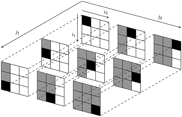
Figure 1. Pseudo-upper triangular tensor.

Definition 15. Identity tensor [15]: An identity tensor $I_N\in {ℂ}^{I_1\times \cdots \times I_N\times I_1\times \cdots \times I_N}$ is a pseudo-diagonal tensor of order 2N such that for any tensor $A\in {ℂ}^{I_1\times \cdots \times I_N\times I_1\times \cdots \times I_N}$, we have $A{*}_N{I}_N=I_N{*}_{N}A=A$ and in which all non-zero entries are 1, i.e.,

$\begin{array}{ll}{(I_N)}_{i_1,i_2,\dots ,i_N,j_1,j_2,\dots ,j_N}={\displaystyle \prod _{k=1}^N{\delta }_{i_k{j}_k}},\text{where }{\delta }_{pq}=\{\begin{array}{l}1,p=q\\ 0,p\ne q.\end{array}& (17)\end{array}$

2.2.2 Transpose, Hermitian, and inverse of a tensor

The transpose of a matrix is a permutation of its two indices corresponding to rows and columns. Since elements of a higher-order tensor are indexed by multiple indices, there are several permutations of such indices, and hence, there can be multiple ways to write the transpose or Hermitian of a tensor. Such permutation-dependent transpose of a tensor is defined in Pan [36].

Assume the set S_N = {1, 2, …, N} and σ is a permutation of S_N. We denote σ(j) = i_j forj = 1, 2, …, N where {i₁, i₂, …, i_N} = {1, 2, …, N} = S_N. Since S_N is a finite set with N elements, it has N! different permutations. Hence, discounting the identity permutation σ(j) = [1, 2, …, N], there are N!−1 different transposes for a tensor with N dimensions or modes. For a tensor $A\in {ℂ}^{I_1\times \cdots \times I_N}$, we define its transpose associated with a certain permutation σ as $A^{T\sigma }\in {ℂ}^{I_{\sigma (1)}\times \cdots \times I_{\sigma (N)}}$ with entries

$\begin{array}{ll}{A}_{i_{\sigma (1)},i_{\sigma (2)},\dots ,i_{\sigma (N)}}^{T\sigma }=A_{i_1,i_2,\dots ,i_N}.& (18)\end{array}$

Similarly, the Hermitian of a tensor $A\in {ℂ}^{I_1\times \cdots \times I_N}$ associated with a permutation σ is defined as the conjugate of its transpose and is denoted as $A^{H\sigma }={(A^{T\sigma })}^{*}\in {ℂ}^{I_{\sigma (1)}\times \cdots \times I_{\sigma (N)}}$ with entries

$\begin{array}{ll}{A}_{i_{\sigma (1)},i_{\sigma (2)},\dots ,i_{\sigma (N)}}^{H\sigma }={(A_{i_{\sigma (1)},i_{\sigma (2)},\dots ,i_{\sigma (N)}}^{T\sigma })}^{*}={(A_{i_1,i_2,\dots ,i_N})}^{*}.& (19)\end{array}$

For example, a transpose of a third-order tensor $X\in {ℂ}^{I_1\times I_2\times I_3}$ such that its third mode is transposed with the first can be written as $X$^Tσ where σ = [3, 2, 1] with components $X_{i_3,i_2,i_1}^{T\sigma }=X_{i_1,i_2,i_3}$. For two tensors $A\in {ℂ}^{I_1\times \cdots \times I_N}$ and $B\in {ℂ}^{I_1\times \cdots \times I_N}$, we have [36]

$\begin{array}{ll}\langle A,B\rangle =\langle A^{T\sigma },B^{T\sigma }\rangle .& (20)\end{array}$

Consider a tensor $Y\in {ℂ}^{I_1\times \cdots \times I_N\times J_1\times \cdots \times J_M}$ and its transposition $Y$^Tσ where the last M modes are swapped with the first N modes. Such a permutation can be denoted as σ = [(N+1), …(N+M), 1, … N] where $Y_{j_1,\dots ,j_M,i_1,\dots i_N}^{T\sigma }=Y_{i_1,\dots ,i_N,j_1,\dots ,j_M}$. Since we will use tensors to define system theory elements with fixed order M output and order N input, the most often encountered case of transpose or Hermitian in this study would be after N modes of an N+M or 2N tensor, i.e., σ = [(N+1), …(N+M), 1, … N]. Henceforth, in such a case we drop the superscript σ for ease of representation and represent such a transpose by $Y$^T and its conjugate by $Y$^H.

Furthermore, a square tensor $U\in {ℂ}^{I_1\times \cdots \times I_N\times I_1\times \cdots \times I_N}$ is called a unitary tensor if $U^H{*}_{N}U=U{*}_N{U}^H=I_N$.

The tensor $A^{-1}\in {ℂ}^{I_1\times \cdots \times I_N\times I_1\times \cdots \times I_N}$ is an inverse of a square tensor of same size, $A\in {ℂ}^{I_1\times \cdots \times I_N\times I_1\times \cdots \times I_N}$ if $A{*}_N{A}^{-1}=A^{-1}{*}_{N}A=I_N$ [28]. The inverse of a tensor exists if its transformation f_{I1, …, IN|I1, …, IN}($A$) is invertible [25]. Several algorithms using the Einstein product such as Higher-order Bi-conjugate Gradient method [25] or Newton's method [37] can be used to find tensor inverse without relying on actually transforming the tensor into a matrix.

As a generalization of the matrix Moore-Penrose inverse, the Moore-Penrose inverse of a tensor $A\in {ℂ}^{I_1\times \cdots \times I_N\times J_1\times \cdots \times J_N}$ is defined as a tensor $A^{+}\in {ℂ}^{J_1\times \cdots \times J_N\times I_1\times \cdots \times I_N}$ that satisfies [27, 38]:

$\begin{array}{l}A{*}_N{A}^{+}{*}_{N}A=A,\\ A^{+}{*}_{N}A{*}_N{A}^{+}=A^{+},\\ {(A{*}_N{A}^{+})}^H=A{*}_N{A}^{+},\\ {(A^{+}{*}_{N}A)}^H=A^{+}{*}_{N}A.\end{array}$

For a tensor $A\in {ℂ}^{I_1\times \cdots \times I_N\times J_1\times \times \cdots \times J_N}$, the Moore-Penrose inverse always exists and is unique [27].

Based on the definition of tensor inverse, Hermitian, and the Einstein product, several tensor algebra relations and properties can be derived. Here, we present a few properties that are often used and can be easily derived:

1. Associativity: For tensors $A\in {ℂ}^{I_1\times \cdots \times I_P\times J_1\times \cdots \times J_N}$, $B\in {ℂ}^{J_1\times \cdots \times J_N\times K_1\times \cdots \times K_M}$, and $C\in {ℂ}^{K_1\times \cdots \times K_M\times T_1\times \cdots \times T_Q}$, we have

$\begin{array}{ll}(A{*}_{N}B){*}_{M}C=A{*}_N(B{*}_{M}C)& (21)\end{array}$

2. Commutativity: The Einstein product is not commutative in all cases. However, for the specific case where the contraction is taken over all the N modes of one of the tensors, say for tensors $A\in {ℂ}^{I_1\times \cdots \times I_P\times J_1\times \cdots \times J_N}$ and $B\in {ℂ}^{J_1\times \cdots \times J_N}$, we get

$\begin{array}{ll}A{*}_{N}B=B{*}_N{A}^T.& (22)\end{array}$

3. Distributivity: For tensors, $A,B\in {ℂ}^{I_1\times \cdots \times I_P\times J_1\times \cdots \times J_N}$ and $C\in {ℂ}^{J_1\times \cdots \times J_N\times K_1\times \cdots \times K_M}$, we have

$\begin{array}{ll}(A+B){*}_{N}C=(A{*}_{N}C)+(B{*}_{N}C).& (23)\end{array}$

4. For tensors $A\in {ℂ}^{I_1\times \cdots \times I_M\times J_1\times \cdots \times J_N}$ and $B\in {ℂ}^{J_1\times \cdots \times J_N\times K_1\times \cdots \times K_P}$, we have

$\begin{array}{ll}{(A{*}_{N}B)}^H=B^H{*}_N{A}^H.& (24)\end{array}$

5. For square invertible tensors $A$ and $B\in {ℂ}^{I_1\times \cdots \times I_N\times I_1\times \cdots \times I_N}$, we have

$\begin{array}{ll}{(A{*}_{N}B)}^{-1}=B^{-1}{*}_N{A}^{-1}.& (25)\end{array}$

2.2.3 Function tensors

A function tensor $A(x)\in {ℂ}_x^{I_1\times \cdots \times I_N}$ is an order N tensor whose components are functions of x. Using a third-order function tensor as an example, each component of $A$(x) is written as $A$_{i, j, k}(x). If x takes discrete values, we represent the function tensor using square bracket notation as $A$[x].

A generalization of the function tensor would be the multivariate function tensor $A(x_1,\dots ,x_p)\in {ℂ}_{x_1,\dots ,x_p}^{I_1\times \cdots \times I_N}$, which is an order N tensor whose components are functions of the continuous variables x₁, …, x_p. If the variables take discrete values, we denote the function tensor as $A$[x₁, ⋯, x_p]. Using the same example of a third-order tensor, each component can be written as $A$_{i, j, k}(x₁, x₂, …, x_p).

A linear system is often expressed as Ax = b where A∈ℂ^M×N is a matrix operating upon the vector x∈ℂ^N to produce another vector b∈ℂ^M [25]. Essentially, the matrix defines a linear operator $L:{ℂ}^N\to {ℂ}^M$ between two vector linear spaces ℂ^N and ℂ^M. A multi-linear system can be thus defined as a linear operator between two tensor linear spaces ${ℂ}^{I_1\times \cdots \times I_N}$ and ${ℂ}^{J_1\times \cdots \times J_M}$, i.e., $\mathrm{ML}:{ℂ}^{I_1\times \cdots \times I_N}\to {ℂ}^{J_1\times \cdots \times J_M}$. Multi-linear systems model several phenomena in various science and engineering applications. However, often in literature, a multi-linear system is degenerated into a linear system by mapping the tensor linear space ${ℂ}^{I_1\times \cdots \times I_N}$ into a vector linear space ${ℂ}^{I_1\cdots I_N}$ through vectorization. The vectorization process allows one to use tools from linear algebra for convenience but also leads to a representation where the distinction between different modes of the system is lost. Thus, possible hidden patterns, structures, and correlations cannot be explicitly identified in the vectorized tensor entities. With the help of tensor contracted product, one can develop signals and system representation without having to rely on vectorization, at the same time extending tools from linear to multi-linear setting intuitively.

2.3 Discrete time signal tensors

A discrete time signal tensor $X\left[n\right]\in {ℂ}_n^{I_1\times \cdots \times I_N}$ is a function tensor whose components are functions of the sampled time index n. A discrete tensor signal can also be called a tensor sequence indexed by n.

A multi-linear time invariant discrete system tensor is an order N + M tensor sequence $H\left[k\right]\in {ℂ}_k^{J_1\times \cdots \times J_M\times I_1\times \cdots \times I_N}$ that couples an input tensor sequence $X\left[k\right]\in {ℂ}_k^{I_1\times \cdots \times I_N}$ of order N with an output tensor sequence $Y\left[k\right]\in {ℂ}_k^{J_1\times \cdots \times J_M}$ of order M through a discrete contracted convolution defined as

$\begin{array}{ll}Y\left[k\right]={\displaystyle \sum _n}{\left\{H\left[n\right],X\left[k-n\right]\right\}}_{\left\{M+1,\dots ,M+N;1,\dots ,N\right\}}.& (26)\end{array}$

Most often the ordering of the modes while defining such system tensors is fixed, where the system tensor contracts over all the input modes. Hence for a more compact notation, we can define the contracted convolution using the Einstein product as

$\begin{array}{ll}Y\left[k\right]={\displaystyle \sum _n}H\left[n\right]{*}_{N}X\left[k-n\right].& (27)\end{array}$

In scalar signals and systems notations, a convolution between two functions is often represented using an asterisk (*). However, to make a distinction with the Einstein product notation which also uses the asterisk symbol, we denote the contracted convolution using the notation •_N, i.e.,

$\begin{array}{ll}Y\left[k\right]=H\left[k\right]{•}_{N}X\left[k\right]={\displaystyle \sum _n}H\left[n\right]{*}_{N}X\left[k-n\right].& (28)\end{array}$

The complex frequency domain representation of discrete signal tensors can be given using the z-transform of the signal tensors, as discussed next.

Definition 16. z-transform of a Discrete Tensor Sequence: The z-transform of $X\left[n\right]\in {ℂ}_n^{I_1\times \dots I_N}$ denoted by $\breve{X}(z)=Z(X[k])\in {ℂ}_z^{I_1\times \dots \times I_N}$ is a tensor of the z-transform of its components defined as

$\begin{array}{ll}\breve{X}(z)=Z(X[k])={\displaystyle \sum _n}X[n]z^{-n}& (29)\end{array}$

with components ${\breve{X}}_{i_1,\dots ,i_N}(z)={\displaystyle \sum _n{X}_{i_1,\dots ,i_N}}[n]z^{-n}.$

The discrete time Fourier transform denoted by $\overline{X}(\omega )=ℱ(X[k])$ of a tensor sequence can be found by substituting z = e^jω in its z-transform as

$\begin{array}{ll}\overline{X}(\omega )=\breve{X}(z){|}_{z=e^{j\omega }}={\displaystyle \sum _n}X[n]z^{-n}{|}_{z=e^{j\omega }}={\displaystyle \sum _n}X[n]e^{-j\omega n}.& (30)\end{array}$

Taking the z-transform of Equation (28), we get

$\begin{array}{l}\breve{Y}(z)={\displaystyle \sum _{k}Y}[k]z^{-k}\\ ={\displaystyle \sum _k\left({\displaystyle \sum _{n}H}[n]{*}_{N}X[k-n]\right)}{z}^{-k}\\ ={\displaystyle \sum _k\left({\displaystyle \sum _{n}H}[n]{*}_{N}X[k-n]\right)}{z}^{n-k}{z}^{-n}\\ ={\displaystyle \sum _{n}H}[n]{*}_N\left({\displaystyle \sum _{k}X}[k-n]z^{n-k}\right)z^{-n}\\ ={\displaystyle \sum _{n}H}[n]z^{-n}{*}_N\breve{X}(z)\\ =\left({\displaystyle \sum _{n}H}[n]z^{-n}\right){*}_N\breve{X}(z)\\ =\breve{H}(z){*}_N\breve{X}(z).& (31)\end{array}$

which shows that the discrete contracted convolution between two tensors in the time domain as given by Equation (28) leads to the Einstein product between the tensors in the z-domain.

2.4 Continuous time signal tensors

A continuous time signal tensor $X(t)\in {ℂ}_t^{I_1\times \cdots \times I_N}$ is a function tensor whose components are functions of the continuous time variable t.

A multi-linear time invariant continuous system tensor is an order N+M tensor $H(t)\in {ℂ}_t^{J_1\times \cdots \times J_M\times I_1\times \cdots \times I_N}$ that couples an order N input continuous tensor signal $X(t)\in {ℂ}_t^{I_1\times \cdots \times I_N}$ with an order M output tensor signal $Y(t)\in {ℂ}_t^{J_1\times \cdots \times J_M}$ through a continuous contracted convolution defined as

$\begin{array}{ll}Y(t)=\int {\left\{H(u),X(t-u)\right\}}_{\left\{M+1,\dots ,M+N;1,\dots ,N\right\}}du.& (32)\end{array}$

In cases where the mode sequence is fixed, similar to the discrete case, we can define a more compact notation using the Einstein product as:

$\begin{array}{ll}Y(t)=H(t){•}_{N}X(t)=\int H(u){*}_{N}X(t-u)du.& (33)\end{array}$

The frequency domain representation of continuous signal tensors can be given using the Fourier transform of the signal tensor as defined next.

Definition 17. Fourier transform: The Fourier transform of $X(t)\in {ℂ}_t^{I_1\times \cdots \times I_N}$ denoted by $\bar{X}(\omega )=F(X(t))$ is a tensor of the Fourier transform of its components defined as

$\begin{array}{ll}\bar{X}(\omega )=F(X(\omega ))=\int X(t)e^{-j\omega t}dt& (34)\end{array}$

with components ${\bar{X}}_{i_1,\dots ,i_N}(\omega )=\int X_{i_1,\dots ,i_N}(t)e^{-i\omega t}dt$.

Using similar line of derivation as for Equation (31), it can be shown that Equation (33) can be written in frequency domain as $\bar{Y}(\omega )=\bar{H}(\omega ){*}_N\bar{X}(\omega )$.

3 Tensor networks

Tensor network (TN) diagrams are a graphical way of illustrating tensor operations [39]. A TN diagram uses a node to represent a tensor, and each outgoing edge from a node represents a mode of the tensor. As such, a vector can be represented through a node with a single edge, a matrix through a node with double edges, and an order N tensor through a node with N edges. This is illustrated in Figure 2. Any form of tensor contraction can be visually presented through a TN diagram.

Figure 2

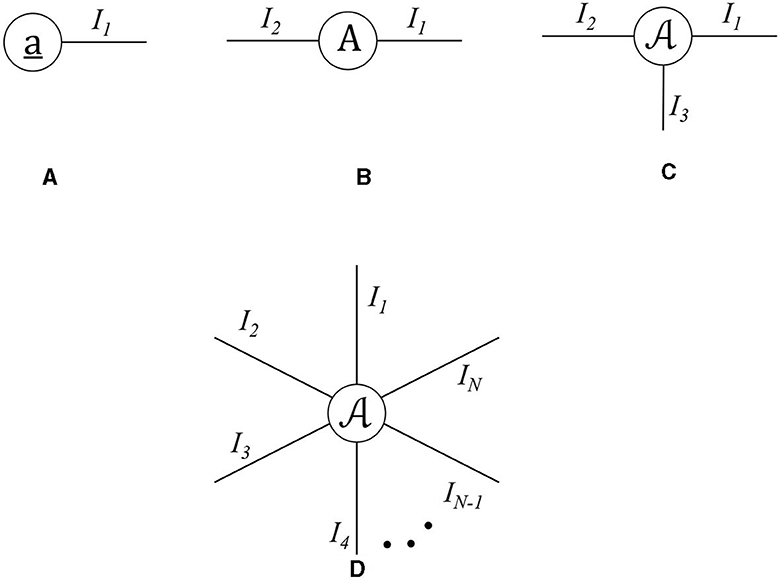
Figure 2. TN diagram representation of (A) vector of size I₁, (B) matrix of size I₁ × I₂, (C) order-3 tensor of size I₁ × I₂ × I₃, and (D) order N tensor of size I₁ × ⋯ × I_N.

3.1 Illustration of contracted products

A contraction between two modes of a tensor is represented in TN by connecting the edges corresponding to the modes that are to be contracted. Hence, the number of free edges represents the order of the resulting tensor. As such any contracted product can be illustrated through a TN diagram, and a few examples are shown in Figure 3. In Figure 3A, the mode-n product of a tensor $A\in {ℂ}^{I_1\times \cdots \times I_N}$ with $\mathrm{\text{U}}\in {ℂ}^{J\times I_n}$, i.e., $A$×_nU from Equation (13) is depicted where the nth edge of $A$ is connected with the second edge of U to represent the contraction of these modes of the same dimension. Figure 3B shows the inner product between two third-order tensors $A$, $B$∈ℂ^I×J×K where all the edges of both the tensors are connected. Since there is no free edge remaining, the result is a scalar. In Figure 3C, a fifth-order tensor $A$∈ℂ^{I×J×K×L×M} contracts with a fourth-order tensor $B$∈ℂ^J×P×L×N along its two common modes as {$A$, $B$}_{{2, 4;1, 3}}. The resulting tensor is an order-5 tensor as there are a total of five free edges in the diagram. Finally, Figure 3D shows the Einstein product between tensors from Equation (9) where the common N modes are connected and we have P+M free edges.

Figure 3

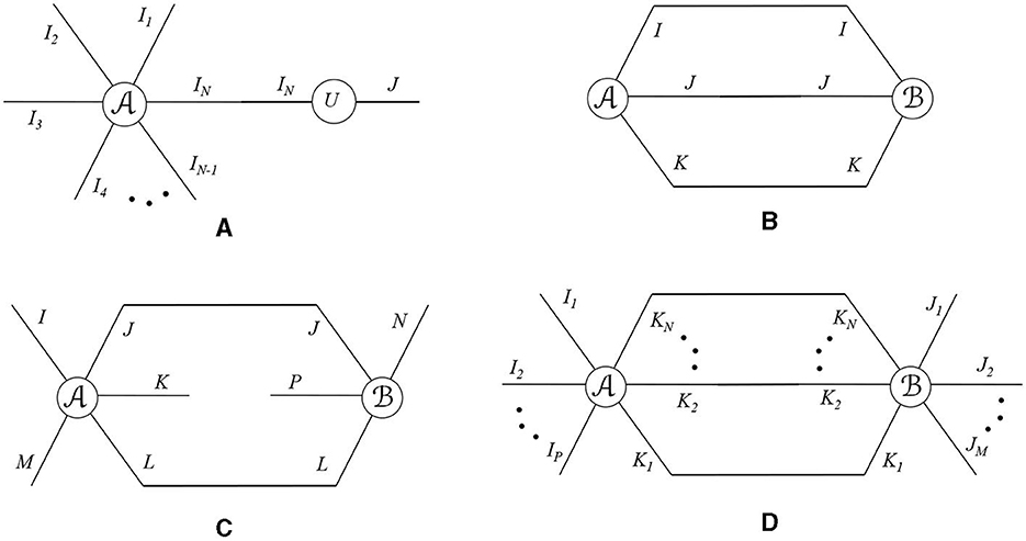
Figure 3. TN representation of contracted product (A) mode-n product between $A\in {ℂ}^{I_1\times \cdots \times I_N}$ and $\mathrm{\text{U}}\in {ℂ}^{J\times I_N}$, (B) between tensor $A$, $B$ ∈ ℂ^I×J×K over all the three modes (inner product), (C) between $A$ ∈ ℂ^{I×J×K×L×M} and $B$ ∈ ℂ^J×P×L×N as {$A$, $B$}_{{2, 4;1, 3}}, and (D) Einstein product between tensors $A\in {ℂ}^{I_1\times \cdots \times I_P\times K_1\times \cdots \times K_N}$ and $B\in {ℂ}^{K_1\times \cdots \times K_N\times J_1\times \cdots \times J_M}$.

3.2 Illustration of contracted convolutions

A contracted convolution is an operation between tensor functions. A function tensor in a TN diagram is represented by a node which is a function of a variable. To represent a function tensor in a TN, we use a rectangular node rather than a circular node. For a given value of the time index k, the contracted convolution from Equation (28) can be depicted using a TN diagram as shown in Figure 4. Note that each $Y$[k] is calculated by computing the Einstein product for all the values of n. Hence, the TN diagram contains a sequence of Einstein product representations between $H$[n] and $X$[k−n]. We suggest a compact representation of the contracted convolution similar to the contracted product, where we connect the edges of the function tensor using a dashed line to represent a contracted convolution as shown in Figure 5. This creates a distinction between the two representations. If the corresponding edges are connected via solid lines, it represents a contracted product, and if they are connected via dashed lines, it represents a contracted convolution.

Figure 4

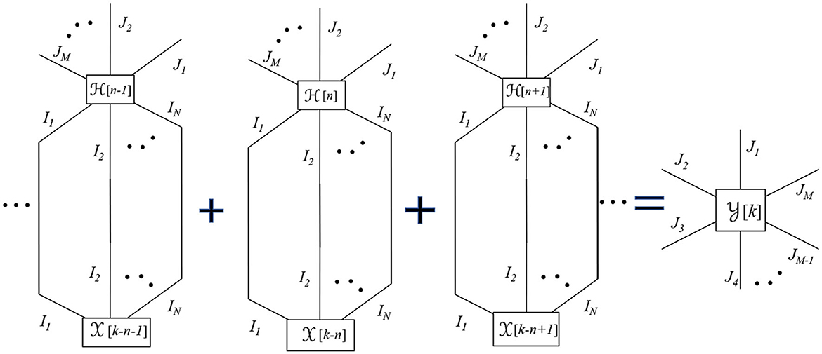
Figure 4. TN representation of contracted convolution from Equation (28).

Figure 5

Figure 5. Compact TN representation of contracted convolution from Equation (28).

To the best of our knowledge, a diagrammatic representation of contracted convolution operation has not been proposed in the literature yet. However, we suggest this representation as it allows an easy way to illustrate multi-domain systems and capture their interactions visually. Note that various contracted products have already been widely depicted in the literature using TN for ease of illustration. Even though a contracted convolution can be seen as a sum of contracted products, depicting it using contracted products in a TN, such as in Figure 4, would lead to a rather complicated representation. Moreover, when considering multiple systems spanning multiple domains interacting with each other, such complicated illustrations would be challenging to interpret and analyze mathematically. Hence, our choice of illustration for contracted convolution in a TN provides an elegant and interpretable visualization of multi-domain systems interaction. In Section 5.3.2, we consider an example of a multi-domain communication system that can be modeled using contracted convolutions, represented through a TN, to illustrate the ease of system representation using our proposed method.

Very often, TN diagrams are used to represent tensor operations as they provide a better visual understanding and thereby aid in developing algorithms to compute tensor operations by making use of elements from graph theory and data structures. Furthermore, a TN diagram can also be used to illustrate how a tensor is formed from several other component tensors. Hence, most tensor decompositions studied in literature are often represented using a TN. In the next section, we discuss some tensor decompositions.

4 Tensor decompositions

Several tensor decompositions such as the Tucker decomposition, Canonical Polyadic (CP) or the Parallel Factor (PARAFAC) decomposition, Tensor Train decomposition, and many more have been extensively studied in the literature [1, 11, 20]. However, in the past decade with the help of Einstein product and its properties, a generalization of matrix SVD and EVD has been proposed in the literature which has found applications in solving multi-linear system of equations and systems theory [18, 25, 26]. In this section, we present some such decompositions using the Einstein product of tensors.

4.1 Tensor singular value decomposition (SVD)

Tucker decomposition of a tensor can be seen as a higher-order SVD [23] and has found many applications, particularly in extracting low-rank structures in higher dimensional data [40]. A more specific version of tensor SVD is explored in Brazell et al. [25] as a tool for finding tensor inversion and solving multi-linear systems. Note that Brazell et al. [25] presents SVD for square tensors only. The idea of SVD from Brazell et al. [25] is further generalized for any even order tensor in Sun et al. [27]. However, it can be further extended for any arbitrary order and size of the tensor. We present a tensor SVD theorem here for any tensor of order N+M.

Theorem 1. For a tensor, $A\in {ℂ}^{I_1\times \cdots \times I_N\times J_1\times \cdots \times J_M}$, the SVD of $A$ has the form:

$\begin{array}{ll}A=U{*}_{N}D{*}_M{V}^H& (35)\end{array}$

where $U\in {ℂ}^{I_1\times \cdots \times I_N\times I_1\times \cdots \times I_N}$ and $V\in {ℂ}^{J_1\times \cdots \times J_M\times J_1\times \cdots \times J_M}$ are unitary tensors, and $D\in {ℂ}^{I_1\times \cdots \times I_N\times J_1\times \cdots \times J_M}$ is a pseudo-diagonal tensor whose non-zero values are the singular values of $A$.

Proof. For tensors $A\in {ℂ}^{I_1\times \cdots \times I_N\times J_1\times \cdots \times J_M}$ and $B\in {ℂ}^{J_1\times \cdots \times J_M\times K_1\times \cdots \times K_P}$, from Equation (14), we get

$\begin{array}{ll}A{*}_{M}B=f_{I_1,\dots ,I_N|K_1,\dots ,K_P}^{-1}\left[f_{I_1,\dots ,I_N|J_1,\dots ,J_M}(A)·f_{J_1,\dots ,J_M|K_1,\dots ,K_P}(B)\right].& (36)\end{array}$

If $\mathrm{\text{A}}\in {ℂ}^{I_1{I}_2\cdots I_N\times J_1{J}_2\cdots J_M}$ and $\mathrm{\text{B}}\in {ℂ}^{J_1{J}_2\cdots J_M\times K_1{K}_2\cdots K_P}$ are transformed matrices from $A$ and $B$, respectively, then substituting f_{I1, …, IN|J1, …, JM}($A$) = A and f_{J1, …, JM|K1, …, KP}($B$) = B in Equation (36) gives us

$\begin{array}{ll}{f}_{I_1,\dots ,I_N|K_1,\dots ,K_P}^{-1}(\text{A}·\text{B})=A{*}_{M}B=f_{I_1,\dots ,I_N|J_1,\dots ,J_M}^{-1}(\text{A}){*}_M{f}_{J_1,\dots ,J_M|K_1,\dots ,K_P}^{-1}(\text{B}).& (37)\end{array}$

Hence if A = U·D·V^H (obtained from matrix SVD), then based on Equation (37), for an order N+M tensor $A\in {ℂ}^{I_1\times \cdots \times I_N\times J_1\times \cdots \times J_M}$, we have

$\begin{array}{l}A=f_{I_1,\dots ,I_N|J_1,\dots ,J_M}^{-1}(\text{A})=f_{I_1,\dots ,I_N|J_1,\dots ,J_M}^{-1}(\text{U}·\text{D}·{\text{V}}^H)\\ =f_{I_1,\dots ,I_N|I_1,\dots ,I_N}^{-1}(\text{U}){*}_N{f}_{I_1,\dots ,I_N|J_1,\dots ,J_M}^{-1}(\text{D}){*}_M{f}_{J_1,\dots ,J_M|J_1,\dots ,J_M}^{-1}({\text{V}}^H)=\\ U{*}_{N}D{*}_M{V}^H.& (38)\end{array}$

Note that for a tensor of order N+M, we will get different SVDs for different values of N and M, but for a given N and M, the SVD is unique which depends on the matrix SVD of f_{I1, …, IN|J1, …, JM}($A$) = A. A proof of this theorem for 2N order tensors with N = M using transformation defined in Equation (6) is provided in [25]. This SVD can be seen as a specific case of Tucker decomposition by expressing the unitary tensors in terms of the factor matrices obtained through Tucker decomposition. Let us consider an example of a fourth-order tensor. For a tensor $A\in {ℂ}^{I_1\times I_2\times K_1\times K_2}$, the Tucker decomposition has the form:

$\begin{array}{ll}A=D{\times }_1{\text{B}}^{(1)}{\times }_2{\text{B}}^{(2)}{\times }_3{\text{B}}^{(3)}{\times }_4{\text{B}}^{(4)}& (39)\end{array}$

where B⁽ⁱ⁾ are factor matrices along all four modes of the tensor and × _n denotes the n-mode product. Now, Equation (39) can be written in matrix form as follows [26]:

$\begin{array}{ll}\begin{array}{l}\text{A}=\underset{\text{U}}{\underbrace{({\text{B}}^{(1)}\otimes {\text{B}}^{(2)})}}·\text{D}·\underset{{\text{V}}^H}{\underbrace{({\text{B}}^{(3)T}\otimes {\text{B}}^{(4)T})}}.\hfill \end{array}& (40)\end{array}$

Now using the transformation from Equation (6), we can map the elements of matrix U to a tensor $U$ as

$\begin{array}{ll}{U}_{i,j,k,l}={\text{U}}_{i+(j-1)I_1,k+(l-1)K_1}.& (41)\end{array}$

Also since U = (B⁽¹⁾ ⊗ B⁽²⁾) and Kronecker product when written element-wise can be expressed as [12]

$\begin{array}{ll}\begin{array}{r}\hfill {\text{U}}_{i+(j-1)I_1,k+(l-1)K_1}={\text{B}}_{j,l}^{(1)}·{\text{B}}_{i,k}^{(2)}\\ \hfill \Rightarrow {\mathcal{U}}_{i,j,k,l}={\text{B}}_{j,l}^{(1)}·{\text{B}}_{i,k}^{(2)}.\end{array}& (42)\end{array}$

This relation can be seen as the unitary tensor $U$ being the outer product of matrices B⁽¹⁾ and B⁽²⁾ [25] but with different mode permutation. Similar relation can be established for $V$ in terms of B⁽³⁾ and B⁽⁴⁾.

4.2 Tensor eigenvalue decomposition (EVD)

As a generalization of matrix eigenvalues to tensors, several definitions exist in the literature for tensor eigenvalues [24]. But most of these definitions apply to super-symmetric tensors which are defined as a class of tensors that are invariant under any permutation of their indices [41]. Such an approach has applications in Physics and Mechanics [41], but there is no single generalization to a higher-order tensor case that preserves all the properties of matrix eigenvalues [21]. Here, we present a particular generalization from Liang et al.[28], Cui et al. [26], and Chen et al. [18] which can be seen as the extension of the matrix spectral decomposition theorem and has applications in multi-linear system theory.

Definition 18. Let $A\in {ℂ}^{I_1\times \cdots \times I_N\times I_1\times \cdots \times I_N},X\in {ℂ}^{I_1\times \cdots \times I_N}$, λ ∈ ℂ, where $X$ and λ satisfy $A$ *_N $X$ = λ$X$, then we call $X$ and λ as eigentensor and eigenvalue of $A$, respectively [26].

Using the definition of Hermitian tensor and tensor eigenvalues, the following lemma can be readily established:

Lemma 2. The eigenvalues of a complex Hermitian tensor $A\in {ℂ}^{I_1\times \cdots \times I_N\times I_1\times \cdots \times I_N}$ are always real.

Theorem 2. The EVD of a Hermitian tensor $A\in {ℂ}^{I_1\times \cdots \times I_N\times I_1\times \cdots \times I_N}$ is given as [25]

$\begin{array}{ll}A=U{*}_{N}D{*}_N{U}^H& (43)\end{array}$

where $U\in {ℂ}^{I_1\times \cdots \times I_N\times I_1\times \cdots \times I_N}$ is a unitary tensor, and $D\in {ℂ}^{I_1\times \cdots \times I_N\times I_1\times \cdots \times I_N}$ is a square pseudo-diagonal tensor, i.e., ${\mathcal{D}}_{i_1,\dots ,i_N,j_1,\dots ,j_N}=0$ if (i₁, …, i_N) ≠ (j₁, …, j_N) with its non-zero values being the eigenvalues of $A$ and $U$ containing the eigentensors of $A$.

This theorem can be proven using Lemma 1, and details are provided in Brazell et al., and Liang et al. [25, 28]. The eigenvalues of $A$ are same as the eigenvalues of $f_{I_1,\dots ,I_N|I_1,\dots ,I_N}(\mathcal{A})$ [42]. We will refer to a tensor $A\in {ℂ}^{I_1\times \cdots \times I_N\times I_1\times \cdots \times I_N}$ as positive semi-definite, denoted by $A$ ≽ 0 if all its eigenvalues are non-negative, which is same as $f_{I_1,\dots ,I_N|I_1,\dots ,I_N}(\mathcal{A})$ being a positive semi-definite matrix. A tensor is positive definite, $A$ ≻ 0, if all its eigenvalues are strictly greater than zero. A positive semi-definite pseudo-diagonal tensor $D$ will have all its components non-negative. Its square root can be denoted as $D$^1/2 which is also pseudo-diagonal positive semi-definite whose elements are the square root of elements of $D$ such that $D^{1/2}{*}_N{D}^{1/2}=D$. Similarly, if $D$ is positive definite, its inverse can be denoted as $D$⁻¹ which is also pseudo-diagonal whose non-zero elements are the reciprocal of the corresponding elements of $D$. Based on tensor EVD, we can also write the square root of any Hermitian positive semi-definite tensor as $A^{1/2}=U{*}_N{D}^{1/2}{*}_N{U}^H$ and inverse of any Hermitian positive definite tensor as $A^{-1}=U{*}_N{D}^{-1}{*}_N{U}^H$. It is straightforward to see that the singular values of a tensor $A\in {ℂ}^{I_1\times \cdots \times I_N\times J_1\times \cdots \times J_M}$ are the square root of the eigenvalues of tensor $A^H{*}_{N}A$. From SVD, if $A=U{*}_{N}D{*}_M{V}^H$, then

$\begin{array}{ll}\begin{array}{c}{\mathcal{A}}^H{*}_N\mathcal{A}=(\mathcal{V}{*}_M{\mathcal{D}}^H{*}_N{\mathcal{U}}^H){*}_N(\mathcal{U}{*}_N\mathcal{D}{*}_M{\mathcal{V}}^H)=\\ \mathcal{V}{*}_M{\mathcal{D}}^H{*}_N\mathcal{D}{*}_M{\mathcal{V}}^H\end{array}& (44)\end{array}$

where $D^H{*}_{N}D$ is the pseudo-diagonal tensor with eigenvalues of $A^H{*}_{N}A$ on its pseudo-diagonal which are square of the singular values obtained from the SVD of $A$.

Definition 19. Trace: The trace of a tensor $A\in {ℂ}^{I_1\times \cdots \times I_N\times I_1\times \cdots \times I_N}$ is defined as the sum of its pseudo-diagonal entries:

$\begin{array}{ll}tr(A)={\displaystyle \sum _{i_1,\dots ,i_N}}{A}_{i_1,i_2,\dots ,i_N,i_1,i_2,\dots ,i_N}.& (45)\end{array}$

Definition 20. Determinant: The determinant of a tensor $A\in {ℂ}^{I_1\times \cdots \times I_N\times I_1\times \cdots \times I_N}$ is defined as the product of its eigenvalues, i.e., if $A=U{*}_{N}D{*}_N{U}^H$, then

$\begin{array}{ll}det(A)={\displaystyle \prod _{i_1,\dots ,i_N}}{D}_{i_1,i_2,\dots ,i_N,i_1,i_2,\dots ,i_N}.& (46)\end{array}$

The eigenvalues of $A$ are the same as that of its matrix transformation, hence $\det (\mathcal{A})=\det (f_{I_1,\dots ,I_N|I_1,\dots ,I_N}(\mathcal{A}))$. Note that there exist other definitions in the literature for determinants based on how one chooses to define the eigenvalues of tensors [43]. The definition presented here is the same as the unfolding determinant in [28].

4.2.1 Some properties of trace and determinant

The following properties can be easily shown by writing the tensors component-wise or using Lemma 1.

1. For two tensors $A\in {ℂ}^{I_1\times \cdots \times I_N}$ and $B\in {ℂ}^{I_1\times \cdots \times I_N}$ of same size and order N,

$\begin{array}{ll}A{*}_{N}B=B{*}_{N}A=tr(A○B)=tr(B○A).& (47)\end{array}$

2. For tensors $A\in {ℂ}^{I_1\times \cdots \times I_N\times J_1\times \cdots \times J_M}$ and $B\in {ℂ}^{J_1\times \cdots \times J_M\times I_1\times \cdots \times I_N}$, we have

$\begin{array}{ll}tr(A{*}_{M}B)=tr(B{*}_{N}A),& (48)\end{array}$

$\begin{array}{ll}det(I_N+A{*}_{M}B)=det(I_M+B{*}_{N}A).& (49)\end{array}$

where $I_N$ and $I_M$ are identity tensors of order 2N and 2M, respectively. To prove Equation (49), we can use Lemma 1 and Sylvester's matrix determinant identity [44].

3. For tensors $A,B\in {ℂ}^{I_1\times \cdots \times I_N\times I_1\times \cdots \times I_N}$, we have

$\begin{array}{ll}det(A{*}_{N}B)=det(B{*}_{N}A)=det(A)·det(B).& (50)\end{array}$

4. Trace of a square tensor is the sum of its eigenvalues.

5. The absolute value of the determinant of a unitary tensor is 1, and the determinant of a square pseudo-diagonal tensor is the product of its pseudo-diagonal entries.

4.3 Tensor LU decomposition

LU decomposition is a powerful tool in linear algebra that can be used for solving systems of equations. In order to solve systems of multi-linear equations, Liang et al. [28] proposed an LU decomposition form for tensors. For $A\in {ℂ}^{I_1\times \cdots \times I_N\times I_1\times \cdots \times I_N}$, the LU factorization takes the form:

$\begin{array}{ll}A=L{*}_{N}U& (51)\end{array}$

where $L,U\in {ℂ}^{I_1\times \cdots \times I_N\times I_1\times \cdots \times I_N}$ are pseudo-lower and pseudo-upper triangular tensors, respectively. In order to solve a system of multi-linear equation $A$ *_N $X$ = $B$ to find $X$, LU decomposition of $A$ can be used to break the equation into two pseudo-triangular equations $U$ *_N $X$ = $Y$ and $L{*}_{N}Y=B$. These two equations can be solved using forward and backward substitution algorithms proposed in Liang et al. [28]. When $B$ is an identity tensor, this method can also be used for finding the inverse of a tensor. More details on computing LU decomposition and the required conditions for its existence can be found in Liang et al. [28].

Note that all these tensor decompositions represent a given tensor in terms of a contracted product between factor tensors. Hence, they all can be represented using tensor network diagrams. For example, we show the TN diagram corresponding to tensor SVD in Figure 6. A detailed TN representation of several other tensor decompositions such as Tucker, PARAFAC, and Tensor Train Decomposition is also presented in Cichocki [39].

Figure 6

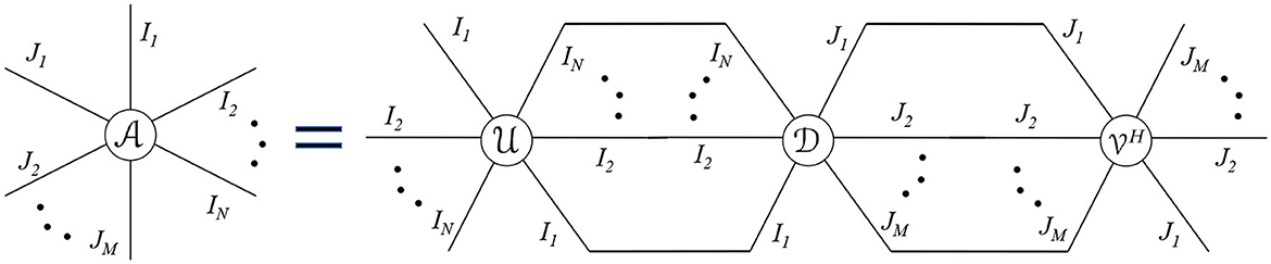
Figure 6. TN representation of tensor SVD from Equation (35).

5 Multi-linear tensor systems

Using the tools presented so far, we will now present the notions of multi-linear system theory using tensors.

5.1 Discrete time multi-linear tensor systems

A discrete time multi-linear tensor system is characterized by an order N + M system tensor $H\left[k\right]\in {ℂ}_k^{J_1\times \cdots \times J_M\times I_1\times \cdots \times I_N}$ which produces an order M output tensor sequence $Y\left[k\right]\in {ℂ}_k^{J_1\times \cdots \times J_M}$ from an input tensor sequence $X\left[k\right]\in {ℂ}_k^{I_1\times \cdots \times I_N}$ through a discrete contracted convolution as defined in Equation (28). The system tensor can be seen as an impulse response tensor whose (j₁, …, j_M, i₁, …, i_N)th entry is the impulse response from the (i₁, …, i_N)th input to the (j₁, …, j_M)th output.

A system tensor is considered p−stable if corresponding to every input of finite p−norm, the system produces an output which is also finite p−norm. When p → ∞, this notion is known as Bounded Input Bounded Output (BIBO) stability. The ∞−norm of a signal tensor $X$ is essentially its peak amplitude evaluated over all the tensor components and all times, i.e.,

$\begin{array}{ll}\Vert X{\Vert }_{\infty }=\underset{k}{\sup }\Vert X[k]{\Vert }_{\infty }=\underset{k}{\sup }\underset{i_1,\dots ,i_N}{\max }\mid X_{i_1,i_2,\mathrm{....},i_N}[k]\mid .& (52)\end{array}$

Theorem 3. For a discrete multi-linear time invariant system with order N input and order M output with an order N + M impulse response system tensor $H\left[k\right]\in {ℂ}_k^{J_1\times \cdots \times J_M\times I_1\times \cdots \times I_N}$, is BIBO stable if and only if

$\begin{array}{ll}\underset{j_1,\dots ,j_M}{\max }{\displaystyle \sum _{i_1,\dots ,i_N}{\displaystyle \sum _k\mid }}{\mathscr{H}}_{j_1,\dots ,j_M,i_1,\dots ,i_N}[k]\mid <\infty .& (53)\end{array}$

Proof. If the input signal tensor $X$[k] satisfies ∥$X$∥_∞ < ∞, then output is given via discrete contracted convolution as

$\begin{array}{ll}Y[k]={\displaystyle \sum _l\mathscr{H}}{[k-l]}_{*N}X[l]& (54)\end{array}$

and thus,

$\begin{array}{l}\underset{j_1,\dots ,j_M}{\max }\mid Y_{j_1,\dots ,j_M}[k]\mid =\\ \underset{j_1,\dots ,j_M}{\max }\mid {\displaystyle \sum _l{\displaystyle \sum _{i_1,\dots ,i_N}{\mathscr{H}}_{j_1,\dots ,j_M,i_1,\dots ,i_N}}}[k-l]X_{i_1,\dots ,i_N}[l]\mid & (55)\end{array}$

$\begin{array}{ll}\le (\underset{j_1,\dots ,j_M}{\max }{\displaystyle \sum _l{\displaystyle \sum _{i_1,\dots ,i_N}\mid }}{\mathscr{H}}_{j_1,\dots ,j_M,i_1,\dots ,i_N}[k-l]\mid )& (56)\end{array}$

$\begin{array}{l}\underset{i_1,\dots ,i_N}{\max }\underset{l}{\sup }\mid X_{i_1,\dots ,i_N}[l]\mid \\ =(\underset{j_1,\dots ,j_M}{\max }{\displaystyle \sum _l{\displaystyle \sum _{i_1,\dots ,i_N}\mid }}{\mathscr{H}}_{j_1,\dots ,j_M,i_1,\dots ,i_N}[k-l]\mid )\Vert X{\Vert }_{\infty }.& (57)\end{array}$

Hence we get,

$\begin{array}{ll}\Vert Y{\Vert }_{\infty }=\underset{k}{\sup }\Vert Y[k]{\Vert }_{\infty }=\underset{k}{\sup }\underset{j_1,\dots ,j_M}{\max }\mid Y_{j_1,\mathrm{....},j_M}[k]\mid & (58)\end{array}$

$\begin{array}{ll}\le (\underset{j_1,\dots ,j_M}{\max }{\displaystyle \sum _{i_1,\dots ,i_N}{\displaystyle \sum _k\mid }}{\mathscr{H}}_{j_1,\dots ,j_M,i_1,\dots ,i_N}[k]\mid )\Vert X{\Vert }_{\infty }<\infty .& (59)\end{array}$

which proves that output is bounded if (53) is satisfied. To prove the converse of the theorem, it suffices to show any example where if (53) is not satisfied, there exists a bounded input which leads to an unbounded output. For this, we can simply consider the case where input and output are scalars which is a special case of the tensor formulation. Equation (53) in that case translates to BIBO condition for SISO LTI system, i.e., $\sum _k\left|h\left[k\right]\right|<\infty$. Hence, it can be readily verified that a signum input defined as x[n] = sgn(h[−n]) which is bounded will lead to an unbounded output if the impulse response sequence is not absolutely summable [45].

           ☐

The BIBO stability condition for a MIMO LTI system requires that every element of the impulse response matrix must be absolutely summable. The condition from Equation (53) can be seen as an extension to the tensor case, where every element of the impulse response tensor must be absolutely summable. Furthermore, we extend the definitions of poles and zeros from matrix-based systems to tensors. A matrix transfer function $\breve{\text{H}}(z)$ has a pole at frequency ν if some entry of $\breve{\text{H}}(z)$ has a pole at z = ν [46]. In addition, $\breve{\text{H}}(z)$ has a zero at frequency γ if the rank of $\breve{\text{H}}(z)$ drops at z = γ [46]. Similarly, a tensor transfer function $\breve{\mathscr{H}}(z)$ has a pole at frequency ν if some entry of $\breve{\mathscr{H}}(z)$ has a pole at z = ν. In addition, $\breve{\mathscr{H}}(z)$ has a zero at frequency γ if the rank of $f_{J_1,\dots ,J_M|I_1,\dots ,I_N}(\breve{\mathscr{H}}(z))$ drops at z = γ. Such a rank is also sometimes referred to as the unfolding rank of the tensor [18, 28].

A tensor system is BIBO stable if all its components are BIBO stable. This implies that every pole of every entry of its transfer function has a magnitude less than 1, i.e., all the poles lie within the unit circle on the z-plane.

5.2 Continuous time multi-linear tensor systems

A continuous time multi-linear tensor system is characterized by an order N + M system tensor $H(t)\in {ℂ}_t^{J_1\times \cdots \times J_M\times I_1\times \cdots \times I_N}$ which produces an order M output tensor signal $Y(t)\in {ℂ}_t^{J_1\times \cdots \times J_M}$ from an input tensor signal $X(t)\in {ℂ}_t^{I_1\times \cdots \times I_N}$ through a contracted convolution as defined in Equation (33). The system tensor can be seen as an impulse response tensor whose (j₁, …, j_M, i₁, …, i_N)th entry is the impulse response from the (i₁, …, i_N)th input to the (j₁, …, j_M)th output.

Similar to the discrete case, a continuous system tensor is considered p−stable if corresponding to every input of finite p−norm, the system produces an output which is also finite p−norm. This notion is known as Bounded Input Bounded Output (BIBO) stability if p = ∞. The ∞−norm of a continuous signal tensor $X$ is essentially its peak amplitude evaluated over all the tensor components and all times, i.e.,

$\begin{array}{ll}\Vert X{\Vert }_{\infty }=\underset{t}{\sup }\Vert X(t){\Vert }_{\infty }=\underset{t}{\sup }\underset{i_1,\dots ,i_N}{\max }\mid X_{i_1,i_2,\mathrm{....},i_N}(t)\mid .& (60)\end{array}$

Theorem 4. For a continuous multi-linear time invariant system with order N input and order M output with an order M + N impulse response system tensor $H(t)\in {ℂ}_t^{J_1\times \cdots \times J_M\times I_1\times \cdots \times I_N}$, is BIBO stable if and only if

$\begin{array}{ll}{\displaystyle \underset{j_1,\dots ,j_M}{max}}{\displaystyle \sum _{i_1,\dots ,i_N}}\int \mid H_{j_1,\dots ,j_M,i_1,\dots ,i_N}(t)\mid dt<\infty .& (61)\end{array}$

The condition from Equation (61) implies that every element of the impulse response tensor must be absolutely integrable. The proof of Theorem 4 follows the same line of proof as of Theorem 3. Furthermore, a continuous system tensor with transfer function $\overline{H}(\omega )$ is BIBO stable if all its components are BIBO stable. This implies that every pole of every entry of its transfer function has a real part less than 0.

5.3 Applications of multi-linear tensor systems

A tensor multi-linear (TML) system can be used to model and represent processes where two tensor signals are coupled through a multi-linear functional. Among various other applications, the use of tensors is ubiquitous in modern communication systems where the signals and systems involved have an inherent multi-domain structure. The physical layer model of modern communication systems invariably spans more than one domain of transmission and reception such as space, time, and frequency to name a few. Consequently, the associated signal processing at the transmitter and receiver has to be cognizant of the multiple domains and their mutual effect on each other for efficient resource utilization. Hence, the signals and the systems involved are best represented using tensors.

5.3.1 System model for multi-domain communication systems

The domains of transmission and reception in modern communication systems depend on specific system configuration. A few examples of possible domains include time slots, sub-carriers, antennas, code sequences, propagation delays, and users. Thus, a generic communication system model which is agnostic to the physical interpretation of the domains, using contracted convolution, was proposed in Venugopal and Leib [15]. Furthermore, a discrete version of the model from Venugopal and Leib [15] using the Einstein product has been proposed in Pandey and Leib [35] where the capacity analysis of higher-order tensor channels is presented.

Consider a multi-domain communication system where the input signal is an order N tensor $X(t)\in {ℂ}_t^{I_1\times \cdots \times I_N}$, which passes through an order M + N multi-linear channel, $H(t)\in {ℂ}_t^{J_1\times \cdots \times J_M\times I_1\times \cdots \times I_N}$. The received signal, or the channel output, in this case can be defined as an order M tensor obtained from the contracted convolution between the channel and the input as Venugopal and Leib [15]:

$\begin{array}{ll}Y(t)=\mathscr{H}(t){•}_{N}X(t)+N(t)& (62)\end{array}$

where $N(t)$ denotes the additive noise tensor of the same size as $Y$(t). Based on the relation between time and frequency domain as discussed in Section 2.4, the frequency domain system model can be specified using the Einstein product as

$\begin{array}{ll}\overline{\mathcal{Y}}(\omega )=\overline{\mathscr{H}}(\omega ){*}_N\overline{\mathcal{X}}(\omega )+\overline{\mathcal{N}}(\omega ).& (63)\end{array}$

Note that such a system model is domain-agnostic and can be used to model several systems. For more illustrative examples, we direct readers to [15] which shows that several systems such as Multi-Input Mulitple-Output (MIMO) Orthogonal Frequency Division Multiplexing (OFDM), Generalized Frequency Division Multiplexing (GFDM), and Frequency Bank Multi-carrier (FBMC) can be modeled using Equation (62). A more detailed discussion on the multi-domain communication system modeling can also be found in Pandey et al.[16] and Pandey and Leib [35]. In this study, we present an example of MIMO Code Division Multiple Access (CDMA) system in Section 5.3.3 modeled using tensor contraction. However, first we show the TN representation of higher-order channels in the next section.

5.3.2 TN representation of TML systems

The channel is expressed as a TML system, and its coupling with the input in both frequency and time domain can be represented in a TN diagram as shown in Figure 7. Note that each edge of the input is connected with the common edge of the channel via a dashed line in the time domain and via a solid line in the frequency domain. Instead of a regular block diagram representation of such systems, the TN diagram has the advantage that it graphically details all the modes of the input and the channel. Thus, just by looking at the free edges of the overall TN diagram, one can determine the modes of the output. The linearity of the system is reflected in the fact that any given edge of the channel is connected with a single edge of the input. Thus, a TML system is easy to identify visually in a TN diagram by observing the presence of one-on-one edge connections between the system and the input.

Figure 7

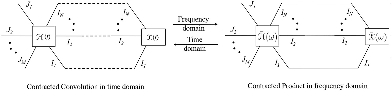
Figure 7. TN representation of TML system in time and frequency domain.

Note that in a communication system, the input signal is often precoded before transmission by a transmit filter and the output signal is processed via a receive filter. The transmit and receiver filters can also be considered system tensors. Thus, the TML channel $H$(t) can be seen as a cascade of three system tensors. Let the transmit filter be represented by $H_T(t)\in {ℂ}_t^{K_1\times \cdots \times K_Q\times I_1\times \cdots \times I_N}$ which transforms the order N input into an order Q transmit signal. The physical channel between the source and destination is modeled as an order P + Q tensor $H_C(t)\in {ℂ}_t^{L_1\times \cdots \times L_P\times K_1\times \cdots \times K_Q}$, and the receive filter is represented by $H_R(t)\in {ℂ}_t^{J_1\times \cdots \times J_M\times L_1\times \cdots \times L_P}$. In this case, the equivalent channel $H$(t) is obtained via a cascade of the three system tensors as

$\begin{array}{ll}\mathscr{H}(t)={\mathscr{H}}_R(t){•}_P{\mathscr{H}}_C(t){•}_Q{\mathscr{H}}_T(t).& (64)\end{array}$

A detailed derivation of such a channel representation can be found in Venugopal and Leib [15]. A cascade of TML systems is conveniently represented in a TN diagram as shown in Figure 8 which illustrates the coupling of the receive filter, physical channel, and transmit filter system tensors in both time and frequency domains. Hence, the nodes for $H$(t) and $\overline{H}(\omega )$ in Figure 7 can be broken down into component system tensors from Figure 8. A tensor system has multiple modes, and the contraction can be along various combinations of such modes. Hence, the TN representation becomes extremely useful as opposed to regular block diagrams, since it allows depiction of the state and coupling of each mode.

Figure 8

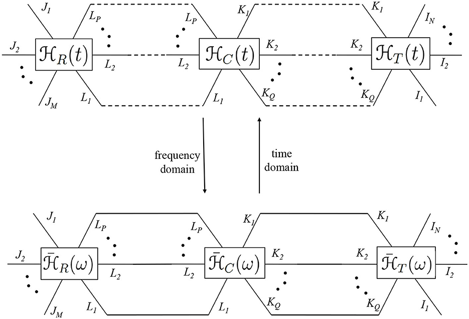
Figure 8. TN representation of equivalent multi-linear channel in time and frequency domain.

5.3.3 Example of Tensor Contraction for MIMO CDMA systems

Code Division Multiple Access (CDMA) is a spread spectrum technique used in communication systems where multiple transmitting users can send information simultaneously over a single communication channel, thereby enabling multiple access. Each user employs the entire bandwidth along with a distinct pseudo-random spreading code to transmit information which is used to distinguish the users at the receiver. More details on CDMA can be found in Proakis and Salehi [47].

Consider an uplink scenario where K users are transmitting information to a single base station (BS). Assume a simple additive white Gaussian Noise (AWGN) channel. Each user is assigned a distinct spreading sequence denoted by vector s^(k) ∈ ℂ^L of length L which transmits a symbol x^(k) for user k. The received signal at the BS can be written as [48]:

$\begin{array}{ll}\underset{\_}{\text{y}}={\displaystyle \sum _{k=1}^K{x}^{(k)}}{\underset{\_}{\text{s}}}^{(k)}+\underset{\_}{\text{z}},& (65)\end{array}$

where z ∈ ℂ^L represents the noise vector. Now consider the extension of such a system model in the presence of flat fading channel and multiple antennas. Assume K users each with N_T transmit antennas are transmitting simultaneously to a BS with N_R receive antennas. To allow multiple access, all the transmit antennas of all different users are assigned different spreading sequences of length L. Let s^{(k, i)} ∈ ℂ^L denotes the length L spreading vector for the data transmitted by the ith antenna of the kth user, x^{(k, i)}. Transmit symbols are assumed to have zero mean and energy $E_s=E\left[|x^{(k,i)}{|}^2\right]$, and the transmit vector from each user and each antenna is generated as x^{(k, i)}s^{(k, i)}. The MIMO communication channel between user k and the BS is defined as a matrix ${\mathrm{\text{H}}}^{(k)}\in {ℂ}^{N_R\times N_T}$ where the random channel matrix has independent and identically distributed (i.i.d.) zero mean circular symmetric complex Gaussian entries with variance 1/N_R. The distribution is denoted as $\mathrm{CN}(0,1/N_R)$. The received signal $\mathrm{\text{Y}}\in {ℂ}^{N_R\times L}$ can be written as [48, 49]:

$\begin{array}{ll}\text{Y}={\displaystyle \sum _{k=1}^K}{\text{H}}^{(k)}{\text{X}}^{(k)}{\text{S}}^{(k)}+\text{Z},& (66)\end{array}$

where X^(k) is an N_T × N_T diagonal matrix defined as $diag(x^{(k,1)},x^{(k,2)},\dots ,x^{(k,N_T)})$ and S^(k) is an N_T × L matrix defined as ${({\underset{\_}{\text{s}}}^{(k,1)T},{\underset{\_}{\text{s}}}^{(k,2)T},\dots ,{\underset{\_}{\text{s}}}^{(k,N_T)T})}^T$. Also Z represents N_R × L noise matrix with i.i.d. components distributed as $\mathrm{CN}(0,N_0)$. In [48], a per-user matched filter receiver is considered for such a system by assuming the interference from other users as noise. It is shown in [48] that such a receiver underperforms as compared to a multi-user receiver which detects the transmit symbols for all the users together. Hence, several multi-user receivers are presented in Nordio and Taricco [48] by rewriting the system model from Equation (66) as

$\begin{array}{ll}\text{Y}=\text{H}\overline{\text{X}}\text{S}+\text{Z},& (67)\end{array}$

where $\mathrm{\text{H}}=({\mathrm{\text{H}}}^{(1)},\dots ,{\mathrm{\text{H}}}^{(K)})\in {ℂ}^{N_R\times K·N_T}$, $\overline{\mathrm{\text{X}}}=diag(x^{(1,1)},\dots ,x^{(1,N_T)},\dots ,x^{(K,1)},\dots ,x^{(K,N_T)})\in {ℂ}^{K·N_T\times K·N_T}$, and $\mathrm{\text{S}}={({\mathrm{\text{S}}}^{(1)T},\dots ,{\mathrm{\text{S}}}^{(K)T})}^T\in {ℂ}^{K·N_T\times L}$. Based on this, a multi-user receiver that aims to mitigate the effects of H (spatial interference) and S (multiple access interference) is considered. The received signal is linearly processed in two stages as Y → AY → AYB, and the transmit signal is decoded as [48]:

$\begin{array}{ll}{\widehat{x}}^{(k,i)}=\underset{x\in D}{\text{arg max}}|{(\text{AYB})}_{j,j}-x{|}^2,\text{\hspace{1em}where }j=(k-1)N_T+i.& (68)\end{array}$

The set $D$ denotes the set of symbols in the transmit constellation map. Essentially AYB represents an estimated version of matrix $\overline{\mathrm{\text{X}}}$, whose diagonal elements at index j are used to decode the transmitted symbols and map them back to index (k, i). The matrices A and B separately aim to mitigate the effects of spatial interference and multiple access interference on the received signal and are defined as

$\begin{array}{ll}\text{A}\triangleq \{\begin{array}{ll}{({\text{H}}^H\text{H})}^{-1}{\text{H}}^H,\hfill & \text{ZF}.\hfill \\ {({\text{H}}^H\text{H}+\frac{N_0}{E_s}{\text{I}}_{K{N}_T})}^{-1}{\text{H}}^H,\hfill & \text{LMMSE}.\hfill \end{array}& (69)\end{array}$

and

$\begin{array}{ll}\text{B}\triangleq \{\begin{array}{ll}{\text{S}}^H{({\text{SS}}^H)}^{-1},\hfill & \text{DECOR}.\hfill \\ {\text{S}}^H{({\text{SS}}^H+\frac{N_0}{E_s}{\text{I}}_{K{N}_T})}^{-1},\hfill & \text{LMMSE}.\hfill \end{array}& (70)\end{array}$

where ${\text{I}}_{K{N}_T}$ is an identity matrix of size K · N_T × K · N_T. The zero forcing (ZF) receiver ignores the impact of noise and only tries to counter the effect of the channel, while the linear minimum mean square error (LMMSE) receiver tries to reduce the noise while simultaneously aiming to mitigate the effect of channel. The DECOR choice represents a multi-user decorrelator receiver. At high SNR value, i.e., as N₀/E_s → 0, the LMMSE option reduces to ZF and DECOR.

Such a receiver based on jointly processing all the users gives better performance than a per-user receiver [48]. However, it still has a drawback in that it tries to combat spatial interference and multiple access interference separately in two stages. Moreover, while the input in Equation (67) is represented as a matrix $\overline{\mathrm{\text{X}}}$, only its diagonal contains the transmit elements which is formed from the concatenation of various x^{(k, i)}. Thus, such a system model does not fully exploit the multi-linearity of the system and tries to force a linear structure by manipulating the entities involved in order to fit the vector-based well-known LMMSE, ZF, or DECOR solutions. In fact, the tensor framework can be ideally used to represent such a system model while keeping the natural structure of the system intact and developing a tensor multi-linear (TML) receiver.

Since the input symbol x^{(k, i)} is indexed by two indices k and i, it is natural to represent the input as a matrix X of size K × N_T with elements ${\mathrm{\text{X}}}_{k,i}=x^{(k,i)}$. Furthermore, the input signal is transmitted as a vector x^{(k, i)} of length L corresponding to each user index k and antenna index i. Hence, the transmitted signal through the channel can be represented as a third-order tensor $X$ of size K × N_T × L where $X_{k,i,l}={\underset{\_}{\text{x}}}_l^{(k,i)}$. To generate $X$ from X, we define the spreading sequences as an order-5 tensor $S\in {ℂ}^{K\times N_T\times L\times K\times N_T}$ with elements $S_{k,i,l,k^{\prime },i^{\prime }}={\underset{\_}{\text{s}}}_l^{(k,i)}$ when k = k′, i = i′, for all l, and 0 elsewhere. Then, we have $X$ = $S$*₂X. Note that here we assume that the elements of X are mapped one to one with a spreading sequence; hence, the entries of $S$ corresponding to k ≠ k′, i ≠ i′ are zero. In certain applications, a linear combination of the input symbols might be transmitted, in which case the structure of $S$ which represents a transmit filtering operation will change accordingly. The channel matrices H^(k) corresponding to each user can be represented as a slice in a third-order tensor $H\in {ℂ}^{N_R\times K\times N_T}$ where $H_{:,k,:}={\mathrm{\text{H}}}^{(k)}$. Thus, the system model can be given as

$\begin{array}{ll}\text{Y}=\underset{\overline{\mathscr{H}}}{\underbrace{\mathscr{H}{*}_{2}S}}{*}_2\text{X}+\text{Z}& (71)\end{array}$

where $\overline{H}\in {ℂ}^{N_R\times L\times K\times N_T}$ represents the equivalent fourth-order TML channel between the order two input X and order two output Y.

Note the advantage of modeling the system model through (71) is that all the associated entities retain their natural structure, and a joint TML receiver can be designed to combat the effect of all the interferences of all the users simultaneously. A multi-linear minimum mean square error receiver that acts across all the domains simultaneously can be represented through a tensor $R\in {ℂ}^{K\times N_T\times N_R\times L}$ which produces an estimate of the input X by acting upon the received tensor Y as $\widetilde{\mathrm{\text{X}}}=R{*}_2\mathrm{\text{Y}}$. Thus, each element of the estimated input at the receiver is a linear combination of all the elements of Y, where the coefficients of the linear combinations are encapsulated in $R$. An optimal choice of $R$ which minimizes the mean square error between X and $\widetilde{\mathrm{\text{X}}}$, defined as $\mathbb{E}\left[\left|\right|\mathrm{\text{X}}-\widetilde{\mathrm{\text{X}}}|{|}_2^2\right]$, is given as [14]:

$\begin{array}{ll}ℛ={\overline{\mathscr{H}}}^H{*}_2{(\overline{\mathscr{H}}{*}_2{\overline{\mathscr{H}}}^H+\frac{N_0}{E_s}ℐ)}^{-1},& (72)\end{array}$

where $I$ is an identity tensor of size K × N_T × K × N_T. The estimated symbol $\widetilde{\mathrm{\text{X}}}$ can be used to detect the transmit symbols as

$\begin{array}{ll}{\widehat{x}}^{(k,i)}=\underset{x\in D}{\text{arg max}}|{\tilde{\text{X}}}_{k,i}-x{|}^2.& (73)\end{array}$

We will refer to such a receiver as a TML MMSE receiver. Since a TML MMSE receiver jointly acts upon symbols across all domains, it aids in detecting the transmit symbol by exploiting the multi-domain interference terms. Through simulation results, we compare the performance of TML MMSE receiver with Equation (68). In Equation (68), we assume A to be the LMMSE matrix from Equation (69), and for B, we simulate both the DECOR and LMMSE matrices from Equation (70). Hence, we simulate LMMSE-DECOR and LMMSE-LMMSE cases from [48]. We will refer to the former as LMMSE1 and the latter as LMMSE2 for our discussion going forward. The simulation parameters used are the same as in Nordio and Taricco [48] where entries of H^(k) are i.i.d. which are $\mathrm{CN}(0,1/N_R)$. It is assumed that the channel realizations are known at the receiver. We assume uncoded transmission with 4QAM modulation where symbols are normalized to have unit energy, i.e., E_s = 1. The spreading sequences are generated with i.i.d. symbols equiprobable over the set {±L^−1/2, ±jL^−1/2}. We use bit error rate (BER) and normalized mean square error (NMSE) as performance measures. All the results are plotted against E_b/N₀ in dB where E_b is the energy per bit defined as E_s/2. Thus, E_b/N₀ represents the received SNR per bit. We perform Monte Carlo simulations where the results are averaged over 100 different channel realizations, and at least 100-bit errors were collected for each SNR to calculate BER. The mean square error is normalized with respect to the number of elements in X and is thus defined as $\mathrm{\text{NMSE}}=\left|\right|\mathrm{\text{X}}-\widetilde{\mathrm{\text{X}}}|{|}_F^2/(N_T·K)$. To compare the performance difference between TML MMSE, LMMSE1, and LMMSE2 against SNR, we plot the BER and NMSE for the three receivers in Figures 9, 10, respectively. We take L = 32, K = 4, N_T = 4, N_R = 32. It can be clearly seen in both the figures that the BER and the NMSE decrease as SNR increases. In particular, the TML MMSE leads to a much lower BER and NMSE compared to the other two receivers as it exploits the multi-linearity of the equivalent channel to jointly combat interference across all the domains. Within LMMSE1 and LMMSE2, it can be observed that LMMSE2 performs better as the choice of DECOR for B from Equation (70) is sub-optimal as compared to LMMSE.

Figure 9

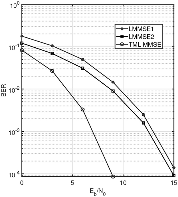
Figure 9. BER performance for different receivers against SNR for L = 32, K = 4, N_R = 32, and N_T = 4.

Figure 10

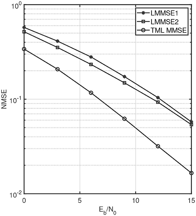
Figure 10. Normalized MSE for different receivers against SNR for L = 32, K = 4, N_T = 32, and N_T = 4.

Furthermore, the advantage of TML MMSE can be clearly seen when BER and NMSE are observed for a fixed SNR per bit and a variable number of users. Consider L = 64, N_R = 64, N_T = 2 and number of users K is variable. Figures 11, 12 present BER and NMSE performance against K for two fixed values of SNR per bit. The solid lines correspond to a 5dB SNR per bit, and dashed lines correspond to an 8dB SNR per bit. It can be clearly seen that for a fixed SNR per bit, the BER and NMSE curves for TML MMSE case remain almost flat as the number of users increases. On the other hand, the performance of LMMSE1 and LMMSE2 significantly degrades with an increase in the number of users. As the number of users increases, the interference across domains also increases which is only efficiently utilized in the TML MMSE receiver.

Figure 11

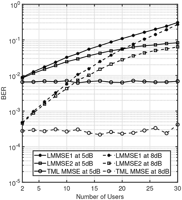
Figure 11. BER performance for different receivers against number of users.

Figure 12

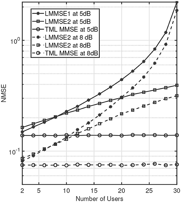
Figure 12. Normalized MSE for different receivers against number of users.

Note that Equation (71) can be re-written as a system of linear equations by using vectorization of the input, output, and noise, and considering the channel as a concatenated matrix $f_{N_R,L|K,N_T}(\overline{H})$. Subsequently, a joint receiver can also be designed using the transformed matrix channel, as presented in Nordio and Taricco [48], which is conceptually equivalent to the TML MMSE approach presented in this study. However, the concatenation of various domains obscures the different domain representations (indices) in the system. Such an approach makes it difficult to incorporate domain-specific constraints at the transceiver. For instance, a common transmit constraint is the power budget which in most practical cases would be different for different users. Thus, designing a transmission scheme with per-user power constraints becomes important and can be achieved using the tensor framework as it maintains the identifiability of domains. Such a consideration has been presented in Pandey et al. [16] and Pandey and Leib [35].

5.3.4 Other examples

In Venugopal and Leib [15], several multi-domain communication systems such as MIMO OFDM, GFDM, and FBMC are represented using the tensor contracted convolution and contracted product. In addition, Venugopal and Leib [15] develops tensor-based receiver equalization methods which are used to combat interference in communication systems using the notion of tensor inversion. A tensor-based receiver and precoder are presented in Pandey and Leib [50] for a MIMO GFDM system where the channel is represented as a sixth-order tensor. The tensor EVD presented in this study is used to design transmit coding operations and perform an information theoretic analysis of the tensor channel [35] leading to the notion of multi-domain water filling power allocation method. In addition, the discrete multi-linear contracted convolution is used to design tensor partial response signaling (TPRS) systems to shape the spectrum and cross-spectrum of transmit signals [16]. The tensor inversion method can also be used to develop estimation techniques for various signal processing applications such as in big data or wireless communications as shown in Pandey and Leib [14]. Another example of the use of tensor Einstein product is for image restoration and reconstruction applications where the objective is to retrieve an image affected by noise, a focal-field distribution, and aperture function [26]. The image data are stored as a three-dimensional tensor, and an order-6 tensor acts as a channel obtained from the point spread function [26], such that output is given using the Einstein product between the input and channel. Another area where the Einstein product properties have been used is the multi-linear dynamical system theory [17, 18]. In Chen et al. [17], a generalized multi-linear time invariant system theory is developed using the Einstein product which can be applied to dynamical systems such as the human genome, social networks, and cognitive sciences. The notion of tensor eigenvalue decomposition presented in this study is used in Chen et al. [17] to derive conditions for stability, reachability, and observability for dynamical systems. The Einstein product has this distinct advantage that it lets us develop tensor algebra notions similar to linear algebra at the same time without disturbing or reshaping the structure of tensors. In addition, the more general tensor contracted product and contracted convolution can be used to model multi-domain systems with any mode ordering as well.

5.3.5 Discussion

The tensor algebra concepts presented in this study provide a structured, intuitive, and mathematically sound framework to characterize and analyze multi-linear systems. Traditionally, matrix-based methods have been used for this purpose by ignoring the signal variability across multiple domains and thereby converting the inherently higher-domain signals and systems into a single concatenated domain with no physical interpretation. Such obfuscated representations are heavily motivated by the ease of employing well-known tools from linear algebra. Several software packages and tools still employ matrix numerical methods for computation. Moreover, since matrix algebra is a standard topic in most engineering programs, engineers are better equipped to handle vectors and matrices than tensors. One primary objective of this study is to provide an easy transition from matrix algebra to tensor algebra for engineering students and researchers. With a proper understanding of the tools from multi-linear algebra, it is straightforward to see the inherent advantages in the tensor formalism. The tensor framework retains the natural structure of the signals and systems involved, thereby capturing the mutual effect of various domains in the system model. The proposed solutions developed with such a framework remain domain-aware and are interpretable.

In addition, sometimes matrix-based representations are offered as a low-complexity solution to tensor-based methods. For instance, in a multi-carrier communication system, a per-subcarrier receive processing using matrix methods is much more computationally efficient as opposed to a tensor-based receiver acting jointly across all users. However, it should be noted that a matrix-based method in itself would not reduce the computational complexity unless some additional assumptions on inter-domain interferences are assumed. For instance, a per-subcarrier receiver assumes zero inter-carrier interference. Without such an assumption, even the degenerate matrix-based formulation of the problem would lead to a large matrix-based model with similar complexity as the equivalent tensor model but with additional loss of distinction between domains. The tensor method provides a structured manner to incorporate all the inter-domain interferences in the system design without resorting to any restructuring. Moreover, the restructuring of data may not be possible in certain applications. With growing big data and IoT applications, even large vector-based data are often stored using tensorization for reducing its storage complexity [39] through tensor train decompositions. Thus, the tensor structure plays a crucial role, and all the mathematical operations for data analysis are expected to be performed while keeping the structure intact. This could be done by resorting to tools from tensor algebra as discussed in this study.

6 Summary and concluding remarks

This study presented a review of tensor algebra concepts developed using the contracted product, more specifically the Einstein product, extending the common notions in linear algebra to a multi-linear setting. In particular, the notion of tensor inverse, singular, and eigenvalue decompositions, LU decomposition were discussed. We also studied the tensor network representations of tensor contractions and convolutions. The notions of time invariant discrete and continuous multi-linear systems which can be defined using the contracted convolutions were also presented. We presented an application in a multi-domain communication system where the channel is modeled as a multi-linear system. The multi-linearity of the channel allowed us to develop a receiver that jointly combats interference across all the domains, thereby giving much better BER and MSE performance as compared to linear receivers which act on a specific domain at a time. The tensor algebra notions discussed in this study have extensive applications in various fields such as communications, signals and systems, controls, and image processing, to name a few. In the presence of several other tensor tutorial studies in literature, this study by no means intends to summarize all the multi-linear algebra concepts but provides an introduction to the main concepts from a signals and systems perspective in a tensor setting.

Author contributions

DP: Investigation, Methodology, Software, Writing—original draft, Writing—review & editing. AV: Investigation, Methodology, Writing—original draft. HL: Conceptualization, Funding acquisition, Investigation, Resources, Supervision, Writing—review & editing.

Funding

The author(s) declare financial support was received for the research, authorship, and/or publication of this article. This work was supported by the Natural Sciences and Engineering Research Council of Canada (NSERC) for project titled “Tensor modulation for space-time-frequency communication systems” under Grant RGPIN-2016-03647.

Conflict of interest

The authors declare that the research was conducted in the absence of any commercial or financial relationships that could be construed as a potential conflict of interest.

Publisher's note

All claims expressed in this article are solely those of the authors and do not necessarily represent those of their affiliated organizations, or those of the publisher, the editors and the reviewers. Any product that may be evaluated in this article, or claim that may be made by its manufacturer, is not guaranteed or endorsed by the publisher.

References

1. Kolda TG, Bader BW. Tensor decompositions and applications. SIAM Review. (2009) 51:455–500. doi: 10.1137/07070111X

Crossref Full Text | Google Scholar

2. Comon P. Tensors: a brief introduction. IEEE Signal Process Mag. (2014) 31:44–53. doi: 10.1109/MSP.2014.2298533

Crossref Full Text | Google Scholar

3. Tucker LR. The extension of factor analysis to three-dimensional matrices. In:Gulliksen H, Frederiksen N, , editors. Contributions to Mathematical Psychology. New York: Holt, Rinehart and Winston (1964). p. 110–27.

Google Scholar

4. Appellof CJ, Davidson ER. Strategies for analyzing data from video fluorometric monitoring of liquid chromatographic effluents. Anal Chem. (1981) 53:2053–6. doi: 10.1021/ac00236a025

Crossref Full Text | Google Scholar

5. Bro R. Review on multiway analysis in Chemistry 2000-2005. Crit Rev Anal Chem. (2006) 36:279–93. doi: 10.1080/10408340600969965

Crossref Full Text | Google Scholar

6. Li X, Ng MK, Ye Y. MultiComm: finding community structure in multi-dimensional networks. IEEE Trans Knowl Data Eng. (2014) 26:929–41. doi: 10.1109/TKDE.2013.48

Crossref Full Text | Google Scholar

7. Papalexakis EE, Faloutsos C, Sidiropoulos ND. Tensors for data mining and data fusion: Models, applications, and scalable algorithms. ACM Trans Intell Syst. (2017) 8:1–44. doi: 10.1145/2915921

Crossref Full Text | Google Scholar

8. Shashua A, Hazan T. Non-negative Tensor Factorization with Applications to Statistics and Computer Vision. In: Proceedings of the 22nd International Conference on Machine Learning. New York, NY: ACM (2005). p. 792–799.

Google Scholar

9. Guerrero JJ, Murillo AC, Sags C. Localization and matching using the planar trifocal tensor with bearing-only data. IEEE Transact Robot. (2008) 24:494–501. doi: 10.1109/TRO.2008.918043

Crossref Full Text | Google Scholar

10. Latchoumane CFV, Vialatte F, Sol-Casals J, Maurice M, Wimalaratna S, Hudson N. et al. Multiway array decomposition analysis of EEGs in Alzheimer's disease. J Neurosci Methods. (2012) 207:41–50. doi: 10.1016/j.jneumeth.2012.03.005

Crossref Full Text | Google Scholar

11. Sidiropoulos ND, Lathauwer LD, Fu X, Huang K, Papalexakis EE, Faloutsos C. Tensor decomposition for signal processing and machine learning. IEEE Transact Signal Process. (2017) 65:3551–82. doi: 10.1109/TSP.2017.2690524

Crossref Full Text | Google Scholar

12. Cichocki A, Mandic D, De Lathauwer L, Zhou G, Zhao Q, Caiafa C, et al. Tensor Decompositions for Signal Processing Applications: From two-way to multiway component analysis. IEEE Signal Process Mag. (2015) 32:145–63. doi: 10.1109/MSP.2013.2297439

Crossref Full Text | Google Scholar

13. Sidiropoulos ND, Bro R, Giannakis GB. Parallel factor analysis in sensor array processing. IEEE Transact Signal Process. (2000) 48:2377–88. doi: 10.1109/78.852018

Crossref Full Text | Google Scholar

14. Pandey D, Leib H, A. Tensor framework for multi-linear complex MMSE estimation. IEEE Open J Signal Process. (2021) 2:336–58. doi: 10.1109/OJSP.2021.3084541

Crossref Full Text | Google Scholar

15. Venugopal A, Leib H, A. Tensor based framework for multi-domain communication systems. IEEE Open J Commun Soc. (2020) 1:606–33. doi: 10.1109/OJCOMS.2020.2987543

Crossref Full Text | Google Scholar

16. Pandey D, Venugopal A, Leib H. Multi-domain communication systems and networks: a tensor-based approach. MDPI Network. (2021) 1:50–74. doi: 10.3390/network1020005

Crossref Full Text | Google Scholar

17. Chen C, Surana A, Bloch A, Rajapakse I. Multilinear time invariant system theory. In: 2019 Proceedings of the Conference on Control and its Applications. Society for Industrial and Applied Mathematics (SIAM) (2019). p. 118–125.

Google Scholar

18. Chen C, Surana A, Bloch AM, Rajapakse I. Multilinear control systems theory. SIAM J Control Optim. (2021) 59:749–76. doi: 10.1137/19M1262589

Crossref Full Text | Google Scholar

19. Chen H, Ahmad F, Vorobyov S, Porikli F. Tensor decompositions in wireless communications and MIMO radar. IEEE J Sel Top Signal Process. (2021) 15:438–53. doi: 10.1109/JSTSP.2021.3061937

Crossref Full Text | Google Scholar

20. Kisil I, Calvi GG, Dees BS, Mandic DP. Tensor Decompositions and Practical Applications: A Hands-on Tutorial. In: Recent Trends in Learning From Data. Cham: Springer (2020). p. 69–97.

Google Scholar

21. Lim LH. Singular values and Eigenvalues of tensors: A variational approach. In: 1st IEEE International Workshop on Computational Advances in Multi-Sensor Adaptive Processing. Puerto Vallarta: IEEE (2005). p. 129–132.

Google Scholar

22. Weiland S, Van Belzen F. Singular Value Decompositions and low rank approximations of tensors. IEEE Trans Signal Process. (2010) 58:1171. doi: 10.1109/TSP.2009.2034308

Crossref Full Text | Google Scholar

23. Lathauwer LD, Moor BD, Vandewalle J. A multilinear singular value decomposition. SIAM J Matrix Anal Appl. (2000) 21:1253–78. doi: 10.1137/S0895479896305696

Crossref Full Text | Google Scholar

24. Qi L. Eigenvalues of a real supersymmetric tensor. J Symbolic Comp. (2005) 40:1302–24. doi: 10.1016/j.jsc.2005.05.007

Crossref Full Text | Google Scholar

25. Brazell M, Li N, Navasca C, Tamon C. Solving multilinear systems via tensor inversion. SIAM J Matrix Analy Appl. (2013) 34:542–70. doi: 10.1137/100804577

Crossref Full Text | Google Scholar

26. Cui LB, Chen C, Li W, Ng MK. An Eigenvalue problem for even order tensors with its applications. Linear Multili Algebra. (2016) 64:602–21. doi: 10.1080/03081087.2015.1071311

Crossref Full Text | Google Scholar

27. Sun L, Zheng B, Bu C, Wei Y. Moore-Penrose inverse of tensors via Einstein product. Linear Multili Algebra. (2016) 64:686–98. doi: 10.1080/03081087.2015.1083933

Crossref Full Text | Google Scholar

28. lin Liang M, Zheng B, juan Zhao R. Tensor inversion and its application to the tensor equations with Einstein product. Linear Multili Algebra. (2019) 67:843–70. doi: 10.1080/03081087.2018.1500993

Crossref Full Text | Google Scholar

29. Huang B, Li W. Numerical subspace algorithms for solving the tensor equations involving Einstein product. Num Linear Algebra Appl. (2021) 28:e2351. doi: 10.1002/nla.2351

Crossref Full Text | Google Scholar

30. Huang B. Numerical study on Moore-Penrose inverse of tensors via Einstein product. Num Algor. (2021) 87:1767–97. doi: 10.1007/s11075-021-01074-0

Crossref Full Text | Google Scholar

31. Huang B, Ma C. An iterative algorithm to solve the generalized Sylvester tensor equations. Linear Multili Algebra. (2018) 2023:1–26. doi: 10.1080/03081087.2023.2176416

Crossref Full Text | Google Scholar

32. Wang QW, Xu X. Iterative algorithms for solving some tensor equations. Linear Multilinear Algebra. (2019) 67:1325–49. doi: 10.1080/03081087.2018.1452889

Crossref Full Text | Google Scholar

33. Bader BW, Kolda TG. Algorithm 862: MATLAB tensor classes for fast algorithm prototyping. ACM Trans Mathemat Softw. (2006) 32:635–53. doi: 10.1145/1186785.1186794

Crossref Full Text | Google Scholar

34. De Lathauwer L, Castaing J, Cardoso JF. Fourth-order cumulant-based blind identification of underdetermined mixtures. IEEE Trans Signal Process. (2007) 55:2965–73. doi: 10.1109/TSP.2007.893943

Crossref Full Text | Google Scholar

35. Pandey D, Leib H. The tensor multi-linear channel and its Shannon capacity. IEEE Access. (2022) 10:34907–44. doi: 10.1109/ACCESS.2022.3160187

Crossref Full Text | Google Scholar

36. Pan R. Tensor transpose and its properties. arXiv [Preprint]. arXiv:1411.1503. (2014). Available online at: https://arxiv.org/abs/1411.1503

Google Scholar

37. Pandey D, Leib H. Tensor multi-linear MMSE estimation using the Einstein product. In: Advances in Information and Communication (FICC 2021). Cham: Springer International Publishing (2021). p. 47–64.

Google Scholar

38. Panigrahy K, Mishra D. Extension of Moore Penrose inverse of tensor via Einstein product. Linear Multilinear Algebra. (2020) 0:1–24. doi: 10.1080/03081087.2020.1748848

Crossref Full Text | Google Scholar

39. Cichocki A. Era of big data processing: A new approach via tensor networks and tensor decompositions. arXiv [Preprint]. arXiv:1403.2048. (2014). Available online at: https://arxiv.org/abs/1403.2048

Google Scholar

40. Zhang A, Xia D. Tensor SVD: Statistical and computational limits. IEEE Trans Inform Theory. (2018) 11: 7311–38. doi: 10.1109/TIT.2018.2841377

Crossref Full Text | Google Scholar

41. Qi L, Chen H, Chen Y. Tensor Eigenvalues and their applications. Cham: Springer (2018).

Google Scholar

42. Luo Z, Qi L, Toint PL. Bernstein concentration inequalities for tensors via Einstein products. arXiv [Preprint]. arXiv:1902.03056. (2019). Available online at: https://arxiv.org/abs/1902.03056

Google Scholar

43. Hu S, Huang ZH, Ling C, Qi L. On Determinants and Eigenvalue theory of tensors. J Symbolic Comp. (2013) 50:508–31. doi: 10.1016/j.jsc.2012.10.001

Crossref Full Text | Google Scholar

44. Petersen KB, Pedersen MS. The Matrix Cookbook. (2012). Available online at: http://www2.compute.dtu.dk/pubdb/pubs/3274-full.html

Google Scholar

45. Mitra SK, Kuo Y. Digital signal processing: a computer-based approach. New York: McGraw-Hill New York. (2006).

Google Scholar

46. Dahleh M, Dahleh MA, Verghese G. Chapter 27: Poles and Zeros of MIMO Systems. In: Lecture Notes on Dynamic Systems and Control. Cambridge MA: MIT OpenCourseWare (2011). Available online at: https://ocw.mit.edu/courses/electrical-engineering-and-computer-science/6-241j-dynamic-systems-and-control-spring-2011/readings/MIT6_241JS11_chap27.pdf

Google Scholar

47. Proakis JG, Salehi M. Fundamentals of Communication Systems. Bangalore: Pearson Education India. (2007).

Google Scholar

48. Nordio A, Taricco G. Linear receivers for the multiple-input multiple-output multiple-access channel. IEEE Trans Commun. (2006) 54:1446–56. doi: 10.1109/TCOMM.2006.878831

Crossref Full Text | Google Scholar

49. Takeuchi K, Tanaka T, Yano T. Asymptotic analysis of general multiuser detectors in MIMO DS-CDMA channels. IEEE J Selected Areas Commun. (2008) 26:486–96. doi: 10.1109/JSAC.2008.080407

Crossref Full Text | Google Scholar

50. Pandey D, Leib H. A tensor based Precoder and Receiver for MIMO GFDM systems. In: ICC 2021 - IEEE International Conference on Communications (held virtually between 14-23 June 2021). Montreal, QC: IEEE (2021). p. 1-6.

Google Scholar