Fitted computational method for singularly perturbed convection-diffusion equation with time delay

A uniformly convergent numerical scheme is proposed to solve a singularly perturbed convection-diffusion problem with a large time delay. The diffusion term of the problem is multiplied by a perturbation parameter, ε. For a small ε, the problem exhibits a boundary layer, which makes it challenging to solve it analytically or using standard numerical methods. As a result, the backward Euler scheme is applied in the temporal direction. Non-symmetric finite difference schemes are applied for approximating the first-order derivative terms, and a higher-order finite difference method is applied for approximating the second-order derivative term. Furthermore, an exponential fitting factor is computed and induced in the difference scheme to handle the effect of the small parameter. Using the discrete maximum principle, the stability of the scheme is examined and analyzed. The developed scheme is parameter-uniform with a linear order of convergence in both space and time. To examine the accuracy of the method, two model examples are considered. Further, the boundary layer behavior of the solutions is given graphically.

1. Introduction

Delay differential equations (DDEs) are differential equations in which the evolution of the system is influenced by its past history. DDEs are called retarded types if the delay argument does not appear in the highest-order derivative term; otherwise, they are neutral types. DDEs play an important role in a variety of fields, including robotics, biosciences [1], economics, epidemiology and mechanics [2], fluid dynamics, reaction-diffusion equations [3], and population dynamics [4].

A singularly perturbed delay differential equation (SPDDE) is a delay differential equation in which its higher-order derivative term is multiplied by a small perturbation parameter (0 < ε ≪ 1) and contains at least one delay parameter on the term different from the highest derivative. In contrast to the magnitude of the delay parameter with the perturbation parameter, the delay is classified as a large delay or a small delay. If the magnitude of the delay parameter of the SPDDE is smaller than the perturbation parameter, then the equation is said to be a singularly perturbed delay differential equation with a small delay, whereas when the magnitude of the delay parameter is higher than the perturbation parameter, it is said to be a singularly perturbed delay differential equation with a large delay [5]. A singularly perturbed problem, which arises as a time delay, occurs in many application areas of science and engineering, for instance, in the simulation of oil extraction from underground reservoirs, chemical processes, fluid flows, water quality problems in river networks, and mechanical systems [6].

The presence of ε as a multiple of the higher-order derivative term causes a boundary layer. The boundary layer is an asymptotically narrow region located in the neighborhood of the endpoints of the domain, where the solution has a steep gradient as ε tends to zero [6]. With the rapidly changing behavior of the solution in the boundary layer, one encounters computational difficulties in treating a singularly perturbed problem using analytically or classical numerical schemes. On the contrary, classical numerical schemes lead to spurious non-physical oscillations in the numerical solution, unless an unacceptably large number of mesh points are considered, which leads to a massive computational cost [7]. In response to this, different authors have to look for sounding numerical schemes which converge uniformly regardless of ε.

Recently, the authors in [8], proposed the implicit-Euler scheme in the time direction and the central difference scheme in the space direction. The authors in [7, 9], proposed the implicit-Euler scheme in the time direction and the hybrid scheme by a proper combination of the midpoint upwind in the outer region and the central difference scheme in the inner region in the spatial direction on the Shishkin mesh. Moreover, this method is addressed in [10], for the two-parameter problem. In [11], the authors proposed the implicit-Euler scheme in the time direction and the hybrid scheme on a generalized Shishkin mesh in the spatial direction. Gowrisankar and Natisan in [12] developed the backward Euler scheme in time direction and the upwind finite difference scheme in the spatial direction using a piecewise uniform mesh. The implicit Euler scheme in the time direction and the upwind scheme in the spatial direction are considered in [13]. In [14], the implicit trapezoidal scheme in the time direction and the hybrid scheme by proper combination of the midpoint upwind in the outer region and the central difference in the inner region in the spatial direction are used.

The implicit Euler scheme in the time direction and the central difference scheme in the space direction are used in [4]. The extended cubic B-spline is considered in [15]. A domain decomposition method is considered in [16, 17]. The authors in [18, 19] proposed hybrid scheme on both Shishkin and Bakhvalov meshes. Podila and Kumar [20] proposed a new stable finite difference scheme on a uniform mesh and also on an adaptive mesh. The backward Euler scheme in the time direction and exponentially fitted difference method is considered in [21]. The Crank-Nicolson method in the time direction and a novel fitted finite difference scheme in spatial direction are proposed in [22]. The Crank-Nicolson method in the time direction and an exponentially fitted spline in the spatial direction are discussed in [23]. The implicit Euler scheme in the time direction and the non-standard finite difference method in the space direction are considered in [24]. In [25], the authors proposed Crank-Nicolson method in the time direction and the operator compact implicit (OCI) method on the Shishkin mesh in the space direction. The backward Euler in the time direction and method of line following Micken's type discretization for the space derivatives are used in [26]. Sahoo and Gupta [27] used higher-order difference with an identity expansion (HODIE) on a piecewise uniform mesh. A similar technique was also used in [28] for a coupled system of singularly perturbed problems. The authors [29, 30] proposed the numerical schemes that work for both cases when the delay term is large or small.

The main aim of this work was to develop a ε-uniform numerical scheme for the class of singularly perturbed convection-diffusion problem with a large time delay. The method comprises the backward Euler scheme in the time direction and an exponentially fitted higher-order finite difference scheme in the spatial direction. Error bound and uniform convergence of the developed scheme is investigated and proved. The proposed scheme gives more accurate, stable, and uniformly convergent results.

In this study, C has been considered as a generic positive constant, which does not depend on Δs, Δt, and ε. The maximum norm is denoted by ‖.‖, which is defined by ‖γ‖ = max_s,t∈Ω|γ(s, t)|.

2. Continuous problem

Let Ω = Ω_s × Ω_t = (0, 1) × (0, 𝕋] for 𝕋 > 0, we consider SPDDE of the form

$\begin{array}{ll}\{\begin{array}{l}{z}_t(s,t)+{𝔏}_{\epsilon }z(s,t)=-\kappa (s,t)z(s,t-\delta )+\gamma (s,t),(s,t)\in \Omega \\ z(s,t)={\psi }_b(s,t),(s,t)\in {\eta }_b=\left[0,1\right]\times \left[-\delta ,0\right],\\ z(0,t)={\psi }_l(t),t\in {\eta }_l=\left\{(0,t):0\le t\le 𝕋\right\},\\ z(1,t)={\psi }_r(t),t\in {\eta }_r=\left\{(1,t):0\le t\le 𝕋\right\},\end{array}& (1)\end{array}$

where 𝔏_εz(s, t) = −εz_ss(s, t) + β(s, t)z_s(s, t) + α(s, t)z(s, t).

Here, ε ∈ (0, 1] and δ > 0 are the perturbation parameter and the delay parameter, respectively. We pretended that the functions β(s, t), α(s, t), κ(s, t), γ(s, t) on $\bar{\Omega }=\left[0,1\right]\times \left[0,𝕋\right]$ and ψ_b(s, t), ψ_l(t), ψ_r(t) on η = η_l ∪ η_r ∪ η_b are smooth enough and bounded which meet α(s, t) ≥ ϖ > 0, κ(s, t) ≥ φ > 0, β(s, t) ≥ μ > 0 on $\bar{\Omega }$. These conditions assure that problem (1) has a boundary layer near s = 1 [7].

2.1. A priori bounds

Under the premises that the data are Hölder continuous and satisfy the following compatibility conditions at the corner points and the delay terms [31], we confirm the existence and uniqueness of the solution of (1)

$\begin{array}{ll}{\psi }_l(0)={\psi }_b(0,0),{\psi }_r(0)={\psi }_b(1,0),& (2)\end{array}$

$\begin{array}{ll}\begin{array}{l}\frac{d{\psi }_l(0)}{dt}-\epsilon \frac{{\partial }^2{\psi }_b(0,0)}{\partial s^2}+\beta (0,0)\frac{\partial {\psi }_b(0,0)}{\partial s}+\\ \alpha (0,0){\psi }_b(0,0)=-\kappa (0,0){\psi }_b(0,-\delta )\\ +\gamma (0,0),\\ \frac{d{\psi }_r(0)}{dt}-\epsilon \frac{{\partial }^2{\psi }_b(1,0)}{\partial s^2}+\beta (1,0)\frac{\partial {\psi }_b(1,0)}{\partial s}+\\ \alpha (1,0){\psi }_b(1,0)=-\kappa (1,0){\psi }_b(1,-\delta )\\ +\gamma (1,0).\end{array}& (3)\end{array}$

These assumptions and conditions are fulfilled. Then, the problem (1) admits a unique solution [31].

Setting ε = 0, the reduced problem of (1) is given as

$\begin{array}{ll}\{\begin{array}{l}\frac{\partial z_0(s,t)}{\partial t}+\beta (s,t)\frac{\partial z_0(s,t)}{\partial s}+\alpha (s,t)z_0(s,t)=-\kappa (s,t)z_0(s,t-\delta )+\gamma (s,t),\\ z_0(s,t)={\psi }_b(s,t),(s,t)\in {\eta }_b,\\ z_0(0,t)={\psi }_l(t),t\in {\bar{\Omega }}_t,\end{array}& (4)\end{array}$

where z₀(s, t) is the solution of the reduced problem.

Lemma 2.1. Let z(s, t) be the solution of (1). Then, we have

$\begin{array}{ll}|z(s,t)-{\psi }_b(s,0)|\le Ct,(s,t)\in \bar{\Omega },& (5)\end{array}$

where C does not depends on ε.

Proof: The proof is considered in [7].

The operator $𝔏=(\frac{\partial }{\partial t}+{𝔏}_{\epsilon })$ in (1) satisfies the next lemma.

Lemma 2.2. (Maximum principle). Let ν(s, t) ∈ C²(Ω) ∪ C⁰(η) satisfies ν(s, t) ≥ 0 (s, t) ∈ η. If 𝔏ν(s, t) ≥ 0, (s, t) ∈ Ω, then $\nu (s,t)\ge 0,(s,t)\in \bar{\Omega }$.

Proof: The proof is considered in [14].

Lemma 2.3. (Stability result). Let z(s, t) be the solution of (1). Then, we have

$\begin{array}{ll}\left|z(s,t)\right|\le {\varpi }^{-1}\Vert \gamma \Vert +max\{|{\psi }_l(t)|,|{\psi }_b(s,t)|,|{\psi }_r(t)|\},& (6)\end{array}$

where ϖ ≤ α(s, t).

Proof: The proof is considered in [22].

Lemma 2.4. The derivative of the solution z(s, t) of (1) with respect to s and t satisfy

$\begin{array}{ll}\begin{array}{l}\left|\frac{{\partial }^{i}z(s,t)}{\partial s^i}\right|\le C\left(1+{\epsilon }^{-i}exp\left(-\frac{\mu (1-s)}{\epsilon }\right)\right),(s,t)\in \bar{\Omega },i=0(1)4,\\ \left|\frac{{\partial }^{l}z(s,t)}{\partial t^l}\right|\le C,(s,t)\in \bar{\Omega },l=0(1)2,\end{array}& (7)\end{array}$

where μ ≤ β(s, t).

Proof: The proof is considered in [7].

3. Numerical scheme

3.1. Temporal semi-discretization

The time domain [0, 𝕋] is discretized uniformly with step size Δt as ${\Omega }_t^M=\left\{t_m=m\Delta t,m=0,1,2,...,M,t_M=𝕋,\Delta t=𝕋/M,\right\}$ and ${\Omega }_t^j=\left\{t_m=m\Delta t,m=0,1,2,...,j,t_j=\delta ,\Delta t=\delta /j,\right\}$ with M + 1 mesh points in [0, 𝕋] and j + 1 mesh points in [−δ, 0]. We have 𝕋 = rδ for some positive integer r.

Applying the backward Euler scheme for time derivative, we get

$\begin{array}{ll}\begin{array}{l}\frac{Z^m(s)-Z^{m-1}(s)}{\Delta t}-\epsilon \frac{d^2{Z}^m(s)}{d{s}^2}+\beta (s,t_m)\frac{d{Z}^m(s)}{ds}+\alpha (s,t_m)Z^m(s)\\ =-\kappa (s,t_m)Z(s,t_{m-\delta })+\gamma (s,t_m).\end{array}& (8)\end{array}$

Simplifying (8), we have

$\begin{array}{ll}{𝔏}^{\Delta t}{Z}^m(s)=\{\begin{array}{l}-\kappa (x,t_m){\psi }_b(s)+\gamma (s,t_m)+\frac{Z^{m-1}(s)}{\Delta t},\\ form=0,1,2,...,j,s\in {\Omega }_s,\\ -\kappa (s,t_m)Z^{m-j}(s)+\gamma (s,t_m)+\frac{Z^{m-1}(s)}{\Delta t},\\ form=j+1,...,M-1,s\in {\Omega }_s,\end{array}& (9)\end{array}$

where ${𝔏}^{\Delta t}{Z}^m(s)=-\epsilon \frac{d^2{Z}^m(s)}{d{s}^2}+\beta (s,t_m)\frac{d{Z}^m(s)}{ds}+P(s,t_m)Z^m(s)$ and $P(s,t_m)=(\frac{1}{\Delta t}+\alpha (s,t_m))$ with the boundaries

$\begin{array}{ll}{Z}^m(0)={\psi }_l(t_m),Z^m(1)={\psi }_r(t_m),m=0(1)M.& (10)\end{array}$

Now, (9) rewrite as

$\begin{array}{ll}{𝔏}^{\Delta t}Z(s)=\{\begin{array}{l}-\kappa (s,t_m){\psi }_b(s)+\gamma (s,t_m)+\frac{Z^{m-1}(s)}{\Delta t},\\ form=0,1,2,...,j,s\in {\Omega }_s,\\ -\kappa (s,t_m)Z^{m-j}(s)+\gamma (s,t_m)+\frac{Z^{m-1}(s)}{\Delta t},\\ form=j+1,...,M-1,s\in {\Omega }_s,\end{array}& (11)\end{array}$

where ${𝔏}^{\Delta t}Z(s)=-\epsilon \frac{d^{2}Z(s)}{d{s}^2}+\beta (s,t_m)\frac{dZ(s)}{ds}+P(s,t_m)Z(s)$ and $Z(s)=Z^m(s)\approx z(s,t_m)$ and $Q(s)=Q^m(s)=Q(s,t_m)$.

The local truncation error in the time direction is given as $e_m(s):=z(s,t_m)-Z^m(s),m=0(1)M.$

Lemma 3.1. The local error e_m at t_m satisfies the bound

$\begin{array}{ll}\Vert e_m\Vert \le C{(\Delta t)}^2.& (12)\end{array}$

Lemma 3.2. The global error E_m at t_m satisfies the bound

$\begin{array}{ll}\Vert E_m\Vert \le C(\Delta t),m=1(1)M-1.& (13)\end{array}$

Proof: Using Lemma 3.1, the global error E_m bound at mth time step is given as

$\begin{array}{l}\begin{array}{l}\Vert E_m\Vert =\Vert {\displaystyle \sum _{l=1}^m}{e}_l\Vert \le \Vert e_1\Vert +\Vert e_2\Vert +\Vert e_3\Vert +...+\Vert e_m\Vert \\ \le C_{1}T(\Delta t),since(m)\Delta t\le T\\ =C(\Delta t),where{C}_{1}T=C,\end{array}\end{array}$

Lemma 3.3. For every m = 0(1)M − 1, the solution Z^m(s) of (9)-(10) satisfies the estimate

$\begin{array}{ll}\left|\frac{d^i{Z}^m(s)}{d{s}^i}\right|\le C\left(1+{\epsilon }^{-i}exp\left(\frac{-\mu }{\epsilon }(1-s)\right)\right),s\in {\bar{\Omega }}_s,i=0(1)4.& (14)\end{array}$

Proof: From (11), $-\epsilon \frac{d^{2}Z(s)}{d{s}^2}+\beta (s,t_m)\frac{dZ(s)}{ds}=g$, where g = Q(s) − P(s, t_m)Z(s).

Now, we integrate twice and we obtain

$\begin{array}{l}Z(s)=Z_P(s)+C_1+C_2{\displaystyle {\int }_s^1}exp(-{\epsilon }^{-1}(B(1)-B(y)))dy,\end{array}$

where $Z_P(s)=-{\int }_s^{1}u(y)dy,u(s)={\int }_s^1{\epsilon }^{-1}g(y)exp(-{\epsilon }^{-1}(B(y)-B(s)))dy,B(s)={\int }_0^s\beta (y)dy.$

Using inequality

$\begin{array}{l}exp(-{\epsilon }^{-1}(B(y)-B(s)))\le exp(-{\epsilon }^{-1}\mu (y-s)),s\le y,\end{array}$

and the bound

$\begin{array}{l}\begin{array}{l}|u(s)|\le C{\epsilon }^{-1}{\displaystyle {\int }_s^1}\left(exp(-{\epsilon }^{-1}\mu (y-s))+C{\epsilon }^{-1}exp(-{\epsilon }^{-1}\mu (1-s))\right)dy\\ \le C\left(1+{\epsilon }^{-2}(1-s)exp(-{\epsilon }^{-1}\mu (1-s))\right).\end{array}\end{array}$

Hence, |Z_p(s)| ≤ C. Here, $Z^{\prime }(1)=-C_2$. The boundary condition Z(1) = 0 yields C₁ = 0. Now, the constants C₁ and C₂ must satisfy

$\begin{array}{l}{C}_2{\displaystyle {\int }_0^1}exp\left(-{\epsilon }^{-1}(B(1)-B(y))\right)dy=-Z_p(0).\end{array}$

Since B(s) is bounded on (0, 1), B(1) − B(y) ≤ C(1 − y). Then,

$\begin{array}{l}{\displaystyle {\int }_0^1}exp\left(-{\epsilon }^{-1}(B(1)-B(y))\right)dy\ge \\ {\displaystyle {\int }_0^1}exp\left(-{\epsilon }^{-1}-\mu (1-y)\right)dy\ge C\epsilon .\end{array}$

It follows that $\left|C_2\right|\le C{\epsilon }^{-1}$. Hence, $\left|Z^{\prime }(1)\right|=\left|C_2\right|\le C{\epsilon }^{-1}$. Finally,

$\begin{array}{l}{Z}^{\prime }(s)=u(s)-C_{2}exp(-{\epsilon }^{-1}(B(1)-B(s)))\end{array}$

implies that

$\begin{array}{l}\left|\frac{dZ(s)}{ds}\right|\le C\left(1+{\epsilon }^{-1}exp\left(\frac{-\mu }{\epsilon }(1-s)\right)\right),s\in {\bar{\Omega }}_s.\end{array}$

The proof is done for i = 1. For i > 1 follows by induction and repeated differentiation. For the details, refer [32].

3.2. Spatial discretization

We discretize the spatial domain [0, 1] into N equal number of sub-intervals with the length of h as 0 = s₀, s₁, ..., s_N = 1, and s_n = nh, n = 0(1)N. Consider a smooth function Z(s) in the interval [0, 1]. From Taylor's series approximation, we get

$\begin{array}{ll}\begin{array}{l}{Z}_{n+1}=Z_n+h{Z}_n^{{}^{\prime }}+\frac{h^2}{2!}{Z}_n^{{}^{″}}+\frac{h^3}{3!}{Z}_n^{{}^{‴}}+\frac{h^4}{4!}{Z}_n^{(4)}+\frac{h^5}{5!}{Z}_n^{(5)}+\frac{h^6}{6!}{Z}_n^{(6)}+\\ \frac{h^7}{7!}{Z}_n^{(7)}+\frac{h^8}{8!}{Z}_n^{(8)}+O(h^9),\\ Z_{n-1}=Z_n-h{Z}_n^{{}^{\prime }}+\frac{h^2}{2!}{Z}_n^{{}^{″}}-\frac{h^3}{3!}{Z}_n^{{}^{‴}}+\frac{h^4}{4!}{Z}_n^{(4)}-\frac{h^5}{5!}{Z}_n^{(5)}+\frac{h^6}{6!}{Z}_n^{(6)}-\\ \frac{h^7}{7!}{Z}_n^{(7)}+\frac{h^8}{8!}{Z}_n^{(8)}-O(h^9).\end{array}& (15)\end{array}$

Following a similar relation of (15), it holds

$\begin{array}{ll}\begin{array}{l}{Z}_{n-1}-2Z_n+Z_{n+1}=\frac{2h^2}{2!}{Z}_n^{{}^{″}}+\frac{2h^4}{4!}{Z}_n^{(4)}+\\ \frac{2h^6}{6!}{Z}_n^{(6)}+\frac{2h^8}{8!}{Z}_n^{(8)}+O(h^{10}),Z_{n-1}^{{}^{″}}-\\ 2Z_n^{{}^{″}}+Z_{n+1}^{{}^{″}}=\frac{2h^2}{2!}{Z}_n^{(4)}+\frac{2h^4}{4!}{Z}_n^{(6)}\\ +\frac{2h^6}{6!}{Z}_n^{(8)}+\frac{2h^8}{8!}{Z}_n^{(10)}+O(h^{12}).\end{array}& (16)\end{array}$

From (16), we have

$\begin{array}{ll}\frac{h^4}{12}{Z}_n^{(6)}=Z_{n-1}^{{}^{″}}-2Z_n^{{}^{″}}+Z_{n+1}^{{}^{″}}-h^2{Z}_n^{(4)}-\frac{2h^6}{6!}{Z}_n^{(8)}-\frac{2h^8}{8!}{Z}_n^{(10)}-O(h^{12}).& (17)\end{array}$

Substituting (17) into (16) and simplifying, we obtain

$\begin{array}{ll}{Z}_{n-1}-2Z_n+Z_{n+1}=\frac{h^2}{30}\left(Z_{n-1}^{{}^{″}}+28Z_n^{{}^{″}}+Z_{n+1}^{{}^{″}}\right)+𝔗,& (18)\end{array}$

where $𝔗=\frac{h^4}{20}{Z}_n^{(4)}-\frac{13h^8}{302,400}{Z}_n^{(8)}+O(h^{10}).$

From (11), we draw

$\begin{array}{ll}-\epsilon \frac{d^{2}Z(s)}{d{s}^2}=-\beta (s,t_m)\frac{dZ(s)}{ds}-P(s,t_m)Z(s)+Q(s),& (19)\end{array}$

where

$\begin{array}{l}Q(s)=\{\begin{array}{l}-\kappa (s,t_m){\psi }_b(s)+\gamma (s,t_m)+\frac{Z^{m-1}(s)}{\Delta t},\\ form=0,1,2,...,j,s\in {\Omega }_s,\\ -\kappa (s,t_m)Z^{m-j}(s)+\gamma (s,t_m)+\frac{Z^{m-1}(s)}{\Delta t},\\ form=j+1,...,M-1,s\in {\Omega }_s.\end{array}\end{array}$

Using (19), we have

$\begin{array}{ll}\begin{array}{l}-\epsilon Z_{n+1}^{{}^{″}}=-\beta (s_{n+1},t_m)Z_{n+1}^{{}^{\prime }}-P(s_{n+1},t_m)Z_{n+1}+Q_{n+1},\\ -\epsilon Z_n^{{}^{″}}=-\beta (s_n,t_m)Z_n^{{}^{\prime }}-P(s_n,t_m)Z_n+Q_n,\\ -\epsilon Z_{n-1}^{{}^{″}}=-\beta (s_{n-1},t_m)Z_{n-1}^{{}^{\prime }}-P(s_{n-1},t_m)Z_{n-1}+Q_{n-1}.\end{array}& (20)\end{array}$

From the Taylor series approximations of $Z_{n-1}^{{}^{\prime }},Z_n^{{}^{\prime }}$ and $Z_{n+1}^{{}^{\prime }}$, we get

$\begin{array}{ll}\begin{array}{l}{Z}_n^{{}^{\prime }}=\frac{Z_{n+1}-Z_{n-1}}{2h},\\ Z_{n+1}^{{}^{\prime }}=\frac{3Z_{n+1}-4Z_n+Z_{n-1}}{2h}-h{Z}_n^{{}^{″}},\\ Z_{n-1}^{{}^{\prime }}=\frac{-Z_{n+1}+4Z_n-3Z_{n-1}}{2h}+h{Z}_n^{{}^{″}}.\end{array}& (21)\end{array}$

Substituting (21) into (20), we have

$\begin{array}{ll}\begin{array}{l}-\epsilon Z_{n+1}^{{}^{″}}=-\beta (s_{n+1},t_m)\left(\frac{3Z_{n+1}-4Z_n+Z_{n-1}}{2h}-h{Z}_n^{{}^{″}}\right)\\ -P(s_{n+1},t_m)Z_{n+1}+Q_{n+1},\\ -\epsilon Z_n^{{}^{″}}=-\beta (s_n,t_m)\frac{Z_{n+1}-Z_{n-1}}{2h}-P(s_n,t_m)Z_n+Q_n,\\ -\epsilon Z_{n-1}^{{}^{″}}=-\beta (s_{n-1},t_m)\left(\frac{-Z_{n+1}+4Z_n-3Z_{n-1}}{2h}+h{Z}_n^{{}^{″}}\right)\\ -P(s_{n-1},t_m)Z_{n-1}+Q_{n-1}.\end{array}& (22)\end{array}$

From (18), we draw

$\begin{array}{ll}-\epsilon \left(\frac{Z_{n-1}-2Z_n+Z_{n+1}}{h^2}\right)=\frac{1}{30}\left(-\epsilon Z_{n-1}^{{}^{″}}-28\epsilon Z_n^{{}^{″}}-\epsilon Z_{n+1}^{{}^{″}}\right)+𝔗.& (23)\end{array}$

Substituting (22) into (23) and rearranging, we obtain

$\begin{array}{l}-\left(\epsilon -\frac{h\beta (s_{n-1},t_m)}{30}+\frac{h\beta (s_{n+1},t_m)}{30}\right)\\ \left(\frac{Z_{n-1}^m-2Z_n^m+Z_{n+1}^m}{h^2}\right)+\frac{\beta (s_{n-1},t_m)}{60h}\left(-3Z_{n-1}^m+4Z_n^m-Z_{n+1}^m\right)+\\ \frac{28\beta (s_n,t_m)}{60h}\left(Z_{n+1}^m-Z_{n-1}^m\right)+\frac{\beta (s_{n+1},t_m)}{60h}\left(Z_{n-1}^m-4Z_n^m+3Z_{n+1}^m\right)+\\ \frac{P(s_{n-1},t_m)}{30}{Z}_{n-1}^m+\frac{28P(s_n,t_m)}{30}{Z}_n^m\\ +\frac{P(s_{n+1},t_m)}{30}{Z}_{n+1}^m=\\ \frac{1}{30}\left(Q_{n-1}^m+28Q_n^m+Q_{n+1}^m\right)+𝔗,& (24)\end{array}$

where

$\begin{array}{ll}{Q}_n^m=\{\begin{array}{l}-\kappa (s_n,t_m){\psi }_b(s_n)+\gamma (s_n,t_m)+\frac{Z_n^{m-1}}{\Delta t},\\ form=0,1,2,...,j,s\in {\Omega }_s,\\ -\kappa (s_n,t_m)Z_n^{m-j}+\gamma (s_n,t_m)+\frac{Z_n^{m-1}}{\Delta t},\\ form=j+1,...,M-1,s\in {\Omega }_s.\end{array}& (25)\end{array}$

3.2.1. Computing the exponential fitting factor

We introduce the exponential fitting factor σ to handle the effect of ε in the layer. From the singular perturbation theory stated in [33], the zero order asymptotic solution of the problem of the form

$\begin{array}{ll}\{\begin{array}{l}-\epsilon Z^{{}^{″}}(s)+\beta (s)Z^{{}^{\prime }}(s)+\alpha (s)Z(s)=q(s),s\in {\Omega }_s=(0,1),\\ Z(0)={\omega }_l,Z(1)={\omega }_r\end{array}& (26)\end{array}$

is given as

$\begin{array}{l}Z(s)\approx Z_0(s)+\frac{\beta (0)}{\beta (s)}\left({\omega }_r-Z_0(1)\right)\\ exp\left(-{\displaystyle {\int }_s^1}\left(\frac{\beta (s)}{\epsilon }-\frac{\alpha (s)}{\beta (s)}\right)ds\right)+O(\epsilon ).& (27)\end{array}$

From Taylor's series, approximation for β(s) and α(s) restricting to their first terms about s = 1 is given as

$\begin{array}{ll}Z(s)\approx Z_0(s)+({\omega }_r-Z_0(1))exp\left(\frac{-\beta (1)(1-s)}{\epsilon }\right),& (28)\end{array}$

where Z₀(s) is the solution of reduced problem. Taking h → 0 and solving (28) at s_n−1, s_n, and s_n+1, we get

$\begin{array}{ll}\begin{array}{l}Z(s_n)\approx Z_0(0)+({\omega }_r-Z_0(1))exp(-\beta (1)(\frac{1}{\epsilon }-n\rho )),\\ Z(s_{n-1})\approx Z_0(0)+({\omega }_r-Z_0(1))exp(-\beta (1)(\frac{1}{\epsilon }-(n-1)\rho )),\\ Z(s_{n+1})\approx Z_0(0)+({\omega }_r-Z_0(1))exp(-\beta (1)(\frac{1}{\epsilon }-(n+1)\rho )),\end{array}& (29)\end{array}$

where $\rho =\frac{h}{\epsilon }$. Multiplying (24) by h and the term containing ε by σ and evaluating the limit of the resulting equation as h → 0, we get

$\begin{array}{c}-\frac{\sigma }{\rho }{\displaystyle \underset{h\to 0}{lim}}(Z_{n-1}^m-2Z_n^m+Z_{n+1}^m)\\ +\frac{\beta (s_{n-1},t_m)}{60}{\displaystyle \underset{h\to 0}{lim}}(-3Z_{n-1}^m+\\ 4Z_n^m-Z_{n+1}^m)+\frac{28\beta (s_n,t_m)}{60}{\displaystyle \underset{h\to 0}{lim}}(Z_{n+1}^m-Z_{n-1}^m)+\\ \frac{\beta (s_{n+1},t_m)}{60}{\displaystyle \underset{h\to 0}{lim}}(Z_{n-1}^m-4Z_n^m+3Z_{n+1}^m)=0.& (30)\end{array}$

From (29), we have

$\begin{array}{ll}\begin{array}{l}{\displaystyle \underset{h\to 0}{lim}}(Z((n-1)h)-2Z(nh)+Z((n+1)h))=\\ ({\omega }_r-Z_0(1))e^{-\beta (1)(\frac{1-s_n}{\epsilon })}(e^{-\beta (1)\rho }+e^{\beta (1)\rho }-2),\\ {\displaystyle \underset{h\to 0}{lim}}(-3Z((n-1)h)+4Z(nh)-Z((n+1)h))=\\ ({\omega }_r-Z_0(1))e^{-\beta (1)(\frac{1-s_n}{\epsilon })}(-3e^{-\beta (1)\rho }-e^{\beta (1)\rho }+4),\\ {\displaystyle \underset{h\to 0}{lim}}(Z((n-1)h)-4Z(nh)+3Z((n+1)h))=\\ ({\omega }_r-Z_0(1))e^{-\beta (1)(\frac{1-s_n}{\epsilon })}(e^{-\beta (1)\rho }+3e^{\beta (1)\rho }-4),\\ {\displaystyle \underset{h\to 0}{lim}}(Z((n+1)h)-Z((n-1)h))=\\ ({\omega }_r-Z_0(1))e^{-\beta (1)(\frac{1-s_n}{\epsilon })}(e^{\beta (1)\rho }-e^{-\beta (1)\rho }).\end{array}& (31)\end{array}$

Substituting (31) into (30) and simplifying yields

$\begin{array}{l}\frac{\sigma }{\rho }\left(e^{\beta (1)\rho }+e^{-\beta (1)\rho }-2\right)=\frac{\beta (s_n,t_m)}{60}\left(30e^{\beta (1)\rho }-30e^{-\beta (1)\rho }\right).\end{array}$

Then, we get the fitting factor σ

$\begin{array}{ll}\sigma =\frac{\rho \beta (s_n,t_m)}{2}coth(\frac{\rho \beta (1)}{2}).& (32)\end{array}$

Therefore, the required scheme is taken as

$\begin{array}{ll}{𝔏}^{\Delta t,h}{Z}_n^m=\frac{1}{30}\left(Q_{n-1}^m+28Q_n^m+Q_{n+1}^m\right),& (33)\end{array}$

where

$\begin{array}{ll}\begin{array}{l}{𝔏}^{\Delta t,h}{Z}_n^m=\\ -\left(\epsilon \sigma -\frac{h\beta (s_{n-1},t_m)}{30}+\frac{h\beta (s_{n+1},t_m)}{30}\right)\\ \left(\frac{Z_{n-1}^m-2Z_n^m+Z_{n+1}^m}{h^2}\right)\\ +\frac{\beta (s_{n-1},t_m)}{60h}\left(-3Z_{n-1}^m+4Z_n^m-Z_{n+1}^m\right)\\ +\frac{28\beta (s_n,t_m)}{60h}\left(Z_{n+1}^m-Z_{n-1}^m\right)\\ +\frac{\beta (s_{n+1},t_m)}{60h}\left(Z_{n-1}^m-4Z_n^m+3Z_{n+1}^m\right)+\frac{P(s_{n-1},t_m)}{30}{Z}_{n-1}^m\\ +\frac{28P(s_n,t_m)}{30}{Z}_n^m+\frac{P(s_{n+1},t_m)}{30}{Z}_{n+1}^m.\end{array}& (34)\end{array}$

In the explicit form, it becomes

$\begin{array}{ll}{R}_n^{-}{Z}_{n-1}^m+R_n^0{Z}_n^m+R_n^{+}{Z}_{n+1}^m=H_n^m,& (35)\end{array}$

where

$\begin{array}{ll}\begin{array}{l}{R}_n^{-}=-\frac{1}{h^2}\left(\epsilon \sigma -\frac{h\beta (s_{n-1},t_m)}{30}+\frac{h\beta (s_{n+1},t_m)}{30}\right)-\\ \frac{3\beta (s_{n-1},t_m)}{60h}+\frac{P(s_{n-1},t_m)}{30}\\ -\frac{28\beta (s_n,t_m)}{60h}+\frac{\beta (s_{n+1},t_m)}{60h},\\ R_n^0=\frac{2}{h^2}\left(\epsilon \sigma -\frac{h\beta (s_{n-1},t_m)}{30}+\frac{h\beta (s_{n+1},t_m)}{30}\right)+\\ \frac{4\beta (s_{n-1},t_m)}{60h}-\frac{4\beta (s_{n+1},t_m)}{60h}\\ +\frac{28P(s_n,t_m)}{30},\\ R_n^{+}=-\frac{1}{h^2}\left(\epsilon \sigma -\frac{h\beta (s_{n-1},t_m)}{30}+\frac{h\beta (s_{n+1},t_m)}{30}\right)-\\ \frac{\beta (s_{n-1},t_m)}{60h}+\frac{28\beta (s_n,t_m)}{60h}\\ +\frac{3\beta (s_{n+1},t_m)}{60h}+\frac{P(s_{n+1},t_m)}{30},\\ H_n^m=\frac{1}{30}\left(Q_{n-1}^m+28Q_n^m+Q_{n+1}^m\right).\end{array}& (36)\end{array}$

3.3. Stability and uniform convergence analysis

Lemma 3.4. (Discrete maximum principle). Assume that $Z_0^m\ge 0,Z_N^m\ge 0$ and ${𝔏}^{\Delta t,h}{Z}_n^m\ge 0,\forall n=1(1)N-1$, then $Z_n^m\ge 0,\forall n=0(1)N$.

Proof: Assume that there is k ∈ {0, 1, 2, …, N}, such that $Z_k^m={min}_{0\le n\le N}{Z}_n^m<0$. Assume that $Z_k^m<0$ and from the assumption, it is shown that k ∉ {0, 1}. So, we have $Z_{k+1}^m-Z_k^m>0$ and $Z_k^m-Z_{k-1}^m<0$. Then, we get ${𝔏}^{\Delta t,h}{Z}_k^m<0$ for k = 1(1)N − 1. So, the assumption $Z_n^m<0\forall n=0(1)N$ is wrong. Therefore, $Z_n^m\ge 0$ and ∀n = 0(1)N.

Lemma 3.5. (Uniform stability result). Let $Z_n^m$ be the solution of (33), then we have

$\begin{array}{l}\left|Z_n^m\right|\le \frac{\Vert {𝔏}^{\Delta t,h}{Z}_n^m\Vert }{\zeta }+max\{|{\psi }_l(t_m)|,|{\psi }_r(t_m)|\},\end{array}$

where P(s_n, t_m) ≥ ζ > 0.

Proof: Let $R=\frac{\Vert {𝔏}^{\Delta t,h}{Z}_n^m\Vert }{\zeta }+max\{|{\psi }_l(t_m)|,|{\psi }_r(t_m)|\}$ and define the barrier functions ${\vartheta }_{n,m}^{\pm }$ by ${\vartheta }_{n,m}^{\pm }=R\pm Z_n^m$. On the boundaries, we get ${\vartheta }_{0,m}^{\pm }=R\pm Z_0^m=\frac{\Vert {𝔏}^{\Delta t,h}{Z}_n^m\Vert }{\zeta }+max\{|{\psi }_l(t_m)|,|{\psi }_r(t_m)|\}\pm$ ψ_l(t_m) ≥ 0 and ${\vartheta }_{N,m}^{\pm }=R\pm Z_N^m=\frac{\Vert {𝔏}^{\Delta t,h}{Z}_n^m\Vert }{\zeta }+max\{|{\psi }_l(t_m)|,|{\psi }_r(t_m)|\}\pm {\psi }_r(t_m)\ge 0$. For s_n, n = 1(1)N − 1, we obtain

$\begin{array}{c}{𝔏}^{\Delta t,h}{\vartheta }_{n,m}=\\ -\left(\epsilon \sigma -\frac{h\beta (s_{n-1},t_m)}{30}+\frac{h\beta (s_{n+1},t_m)}{30}\right)\left(\frac{R\pm Z_{n-1}^m-2(R\pm Z_n^m)+R\pm Z_{n+1}^m}{h^2}\right)\\ +\frac{\beta (s_{n-1},t_m)}{60h}\left(-3(R\pm Z_{n-1}^m)+4(R\pm Z_n^m)-(R\pm Z_{n+1}^m)\right)\\ +\frac{28\beta (s_n,t_m)}{60h}\left(R\pm Z_{n+1}^m-(R\pm Z_{n-1}^m)\right)\\ +\frac{\beta (s_{n+1},t_m)}{60h}\left(R\pm Z_{n-1}^m-4(R\pm Z_n^m)+3(R\pm Z_{n+1}^m)\right)\\ +\frac{P(s_{n-1},t_m)}{30}\left(R\pm Z_{n-1}^m\right)+\frac{28P(s_n,t_m)}{30}\left(R\pm Z_n^m\right)+\\ \frac{P(s_{n+1},t_m)}{30}\left(R\pm Z_{n+1}^m\right)\\ =\left(\frac{P(s_{n-1},t_m)}{30}+\frac{28P(s_n,t_m)}{30}+\frac{P(s_{n+1},t_m)}{30}\right)R\pm {𝔏}^{\Delta t,h}{Z}_n^m\\ =\left(\frac{P(s_{n-1},t_m)}{30}+\frac{28P(s_n,t_m)}{30}+\frac{P(s_{n+1},t_m)}{30}\right)\\ (\frac{\Vert {𝔏}^{\Delta t,h}{Z}_n^m\Vert }{\zeta }\\ +max\{|{\psi }_l(t_m)|,|{\psi }_r(t_m)|\})\\ \pm \frac{1}{30}\left(Q_{n-1}^m+28Q_n^m+Q_{n+1}^m\right)\ge 0.& (37)\end{array}$

By Lemma 3.4, we get ${\vartheta }_{n,m}^{\pm }\ge 0,n=0(1)N$. Therefore, the needed bound is obtained.

From Taylor's series expansion, we get

$\begin{array}{c}\left|-\left(\frac{d}{d{s}^2}-{\delta }_s^2\right)Z^m(s_n)\right|\\ \le C{h}^2\Vert \frac{d^4{Z}^m(s_n)}{d{s}^4}\Vert ,\\ \left|\frac{d{Z}^m(s_{n-1})}{ds}-\left(\frac{-Z_{n+1}^m+4Z_n^m-3Z_{n-1}^m}{2h}+h\frac{d^2{Z}^m(s_n)}{d{s}^2}\right)\right|\\ \le C{h}^2\Vert \frac{d^3{Z}^m(s_n)}{d{s}^3}\Vert ,\\ \left|\frac{d{Z}^m(s_{n+1})}{ds}-\left(\frac{3Z_{n+1}^m-4Z_n^m+Z_{n-1}^m}{2h}-h\frac{d^2{Z}^m(s_n)}{d{s}^2}\right)\right|\\ \le C{h}^2\Vert \frac{d^3{Z}^m(s_n)}{d{s}^3}\Vert ,\\ \left|(\frac{d}{ds}-{\delta }_s^0)Z^m(s_n)\right|\le C{h}^2\Vert \frac{d^3{Z}^m(s_n)}{d{s}^3}\Vert ,\\ \left|{\delta }_s^2{Z}^m(s_n)\right|\le C\Vert \frac{d^2{Z}^m(s_n)}{d{s}^2}\Vert ,& (38)\end{array}$

where $\Vert Z^{(k)}(s_n)\Vert ={max}_{s_n\in (s_0,s_N)}|Z_m^{(k)}(s_n)|,k=2,3,4.$

The next theorem provides the truncation error estimate for the developed scheme.

Theorem 3.6. Let the coefficients α(s, t_m), β(s, t_m), and κ(s, t_m) of (9)-(10) be sufficiently smooth such that Z^m(s) ∈ C⁴[0, 1]. Then, the solution $Z_n^m$ of (33) satisfies the next bound

$\begin{array}{ll}\left|{𝔏}^{\Delta t,h}(Z^m(s_n)-Z_n^m)\right|\le \frac{C{h}^2}{h+\epsilon }\left(1+{\epsilon }^{-3}exp\left(\frac{-\mu (1-s_n)}{\epsilon }\right)\right).& (39)\end{array}$

Proof: The error estimate in the spatial direction is given as

$\begin{array}{ll}\begin{array}{l}\left|{𝔏}^{\Delta t,h}(Z^m(s_n)-Z_n^m)\right|=\\ |-\epsilon \left(\frac{d}{d{s}^2}-\sigma {\delta }_s^2\right)Z^m(s_n)+\frac{\beta (s_{n-1},t_m)}{30}\\ \left(\frac{d{Z}^m(s_{n-1})}{ds}-\left(\frac{-Z_{n+1}^m+4Z_n^m-3Z_{n-1}^m}{2h}+h\frac{d^2{Z}^m(s_n)}{d{s}^2}\right)\right)\\ +\frac{28\beta (s_n,t_m)}{30}\left(\frac{d}{ds}-{\delta }_s^0\right)Z^m(s_n)+\frac{\beta (s_{n+1},t_m)}{30}\\ \left(\frac{d{Z}^m(s_{n+1})}{ds}-\left(\frac{3Z_{n+1}^m-4Z_n^m+Z_{n-1}^m}{2h}-h\frac{d^2{Z}^m(s_n)}{d{s}^2}\right)\right)|\\ \le \left|\epsilon (\beta (s_n,t_m)\frac{\rho }{2}coth(\beta (1)\frac{\rho }{2})-1){\delta }_s^2{Z}^m(s_n)\right|\\ +|\epsilon \left(\frac{d^2}{d{s}^2}-{\delta }_s^2\right)Z^m(s_n)|+|\frac{\beta (s_{n-1},t_m)}{30}\\ \left(\frac{d{Z}^m(s_{n-1})}{ds}-\left(\frac{-Z_{n+1}^m+4Z_n^m-3Z_{n-1}^m}{2h}+h\frac{d^2{Z}^m(s_n)}{\partial s^2}\right)\right)|\\ +\left|\frac{28\beta (s_n,t_m)}{30}\left(\frac{d}{ds}-{\delta }_s^0\right)Z^m(s_n)\right|+|\frac{\beta (s_{n+1},t_m)}{30}\\ \left(\frac{d{Z}^n(s_{n+1})}{ds}-\left(\frac{3Z_{n+1}^m-4Z_n^m+Z_{n-1}^m}{2h}-h\frac{d^2{Z}^m(s_n)}{d{s}^2}\right)\right)|,\end{array}& (40)\end{array}$

where $\sigma =\beta (s_n,t_m)\frac{\rho }{2}coth(\beta (1)\frac{\rho }{2})$ and $\rho =\frac{h}{\epsilon }$.

For the constants C₁ and C₂, we have $\left|\rho coth(\rho )-1\right|\le C_1{\rho }^2$ for ρ ≤ 1. For ρ → ∞, since ${lim}_{\rho \to \infty }coth(\rho )=1$ which gives |ρ coth(ρ) − 1| ≤ C₁ρ.

Generally, ∀ρ > 0, we express as

$\begin{array}{ll}{C}_1\frac{{\rho }^2}{\rho +1}\le \rho coth(\rho )-1\le C_2\frac{{\rho }^2}{\rho +1}& (41)\end{array}$

and we have

$\begin{array}{ll}\epsilon [\beta (s_n,t_m)\frac{\rho }{2}coth(\beta (1)\frac{\rho }{2})-1]\le \epsilon \frac{{(h/\epsilon )}^2}{h/\epsilon +1}=\frac{h^2}{h+\epsilon }.& (42)\end{array}$

From the bounds in (38), (40), and (42), we have

$\begin{array}{l}\left|{𝔏}^{\Delta t,h}(Z^m(s_n)-Z_n^m)\right|\le \frac{C{h}^2}{h+\epsilon }\Vert \frac{d^2{Z}^m(s_n)}{d{s}^2}\Vert +C{h}^2\Vert \frac{d^3{Z}^m(s_n)}{d{s}^3}\Vert \\ +C\epsilon h^2\Vert \frac{d^4{Z}^m(s_n)}{d{s}^4}\Vert .\end{array}$

By Lemma 3.3, we have

$\begin{array}{ll}\begin{array}{l}\left|{𝔏}^{\Delta t,h}(Z^m(s_n)-Z_n^m)\right|\le \frac{C{h}^2}{h+\epsilon }\left(1+{\epsilon }^{-2}exp\left(-\frac{\mu (1-s_n)}{\epsilon }\right)\right)\\ +C{h}^2[\left(1+{\epsilon }^{-3}exp\left(-\frac{\mu (1-s_n)}{\epsilon }\right)\right)\\ +\left(\epsilon +{\epsilon }^{-3}exp\left(-\frac{\mu (1-s_n)}{\epsilon }\right)\right)].\end{array}& (43)\end{array}$

Obviously, ε⁻³ ≥ ε⁻², then we draw

$\begin{array}{ll}\left|{𝔏}^{\Delta t,h}(Z^m(s_n)-Z_n^m)\right|\le \frac{C{h}^2}{h+\epsilon }\left(1+{\epsilon }^{-3}exp\left(\frac{-\mu (1-s_n)}{\epsilon }\right)\right)& (44)\end{array}$

thus, it gives the wanted bound.

Lemma 3.7. For a fixed mesh and as ε → 0, it holds

$\begin{array}{r}{\displaystyle \underset{\epsilon \to 0}{lim}}{\displaystyle \underset{i}{max}}\frac{exp(-\mu s_n/\epsilon )}{{\epsilon }^i}=0,\\ {\displaystyle \underset{\epsilon \to 0}{lim}}{\displaystyle \underset{i}{max}}\frac{exp(-\mu (1-s_n)/\epsilon )}{{\epsilon }^i}=\\ 0,i=1,2,3,...,\end{array}$

where s_n = nh, 1 ≤ n ≤ N − 1.

Proof: The proof is in [22].

Theorem 3.8. Let $Z_n^m$ be the solution of (33), then we have the following uniform error bound

$\begin{array}{ll}{\displaystyle \underset{\epsilon \in (0,1]}{sup}}{\displaystyle \underset{n}{max}}\left|Z^m(s_n)-Z_n^m\right|\le Ch,n=0(1)N.& (45)\end{array}$

Proof: Substituting Lemma 3.7 into (39), we arrive at

$\begin{array}{ll}\left|{𝔏}^{\Delta t,h}(Z^m(s_n)-Z_n^m)\right|\le \frac{C{h}^2}{h+\epsilon }.& (46)\end{array}$

Hence, the result leads

$\begin{array}{ll}\left|Z^m(s_n)-Z_n^m\right|\le \frac{C{h}^2}{h+\epsilon }.& (47)\end{array}$

Using the sup over all ε ∈ (0, 1], we get

$\begin{array}{ll}{\displaystyle \underset{\epsilon \in (0,1]}{sup}}{\displaystyle \underset{n}{max}}\left|Z^m(s_n)-Z_n^m\right|\le Ch,n=0(1)N.& (48)\end{array}$

From (46), when ε > h, the obtained method uniformly converges uniformly with order two in the space direction. When ε ≪ h, the method converges uniformly with order one in the space direction.

Theorem 3.9. Let z and Z are the solutions of (1) and (33), respectively, then we have the following uniform error bound

$\begin{array}{ll}{\displaystyle \underset{\epsilon \in (0,1]}{sup}}\left|z-Z\right|\le C(h+(\Delta t)).& (49)\end{array}$

Proof: The proof is considered by combining of Lemma 3.1 and Theorem 3.8.

4. Numerical results

Considering two test examples we carry out some numerical inquiries to confirm the developed scheme is ε-uniform convergent. Since the exact solution of the examples are not known, we used a variant of double mesh principle is applied for the numerical inquiries. So, we calculate the maximum pointwise error by $E_{\epsilon }^{N,M}={max}_{n,m}\left|Z_{n,m}^{N,M}-Z_{n,m}^{2N,2M}\right|$, the ε-uniform error by $E^{N,M}={max}_{n,m}(E_{\epsilon }^{N,M})$, the rate of convergence by $r_{\epsilon }^{N,M}=log2(E_{\epsilon }^{N,M}/E_{\epsilon }^{2N,2M}),$ and the ε-uniform rate of convergence by r^N,M = log2(E^N,M/E^{2N, 2M}).

4.1. Example

Consider the problem [7]

$\begin{array}{l}\frac{\partial z}{\partial t}-\epsilon \frac{{\partial }^{2}z}{\partial s^2}+(2-s^2)\frac{\partial z}{\partial s}+su(s,t)+u(s,t-\delta )=\\ 10t^{2}exp(-t)s(1-s),\end{array}$

(s, t) ∈ (0, 1) × (0, 2] with interval condition z(s, t) = 0, on (s, t) ∈ [0, 1] × [−1, 0] and the boundary conditions z(0, t) = 0 and z(1, t) = 0, t ∈ [0, 2].

4.2. Example

Consider the problem [13]

$\begin{array}{r}\frac{\partial z}{\partial t}-\epsilon \frac{{\partial }^{2}z}{\partial s^2}+(2-s^2)\frac{\partial z}{\partial s}+(s+1)(t+1)z(s,t)+z(s,t-\delta )=\\ 10t^{2}exp(-t)s(1-s),\end{array}$

(s, t) ∈ (0, 1) × (0, 2] with interval condition z(s, t) = 0, on (s, t) ∈ [0, 1] × [−1, 0] and the boundary conditions z(0, t) = 0 and z(1, t) = 0, t ∈ [0, 2].

For distinguishable values of ε and N, the obtained results for the model Examples 4.1 and 4.2, respectively, $E_{\epsilon }^{N,M},E^{N,M}$, $r_{\epsilon }^{N,M}$, and r^N,M of the developed scheme are delineated in Tables 1, 2. From these tables, one can observe that the maximum absolute error decreases as the step sizes decrease for every value of ε, and as ε approaches to zero, the maximum absolute error after getting large becomes constant, which displays ε-uniform convergence of the proposed scheme regardless of ε. On the other hand, the calculated E^N,M and the corresponding r^N,M using the proposed scheme are given in the last two rows, which confirms that the theoretical finding of the developed scheme is order one in both space and time direction.

TABLE 1

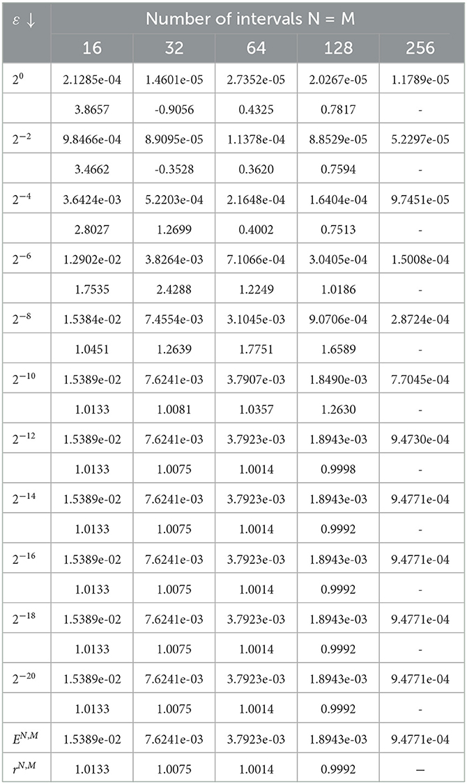
Table 1. $E_{\epsilon }^{N,M},E^{N,M},r_{\epsilon }^{N,M}$, and r^N,M for Example 4.1.

TABLE 2

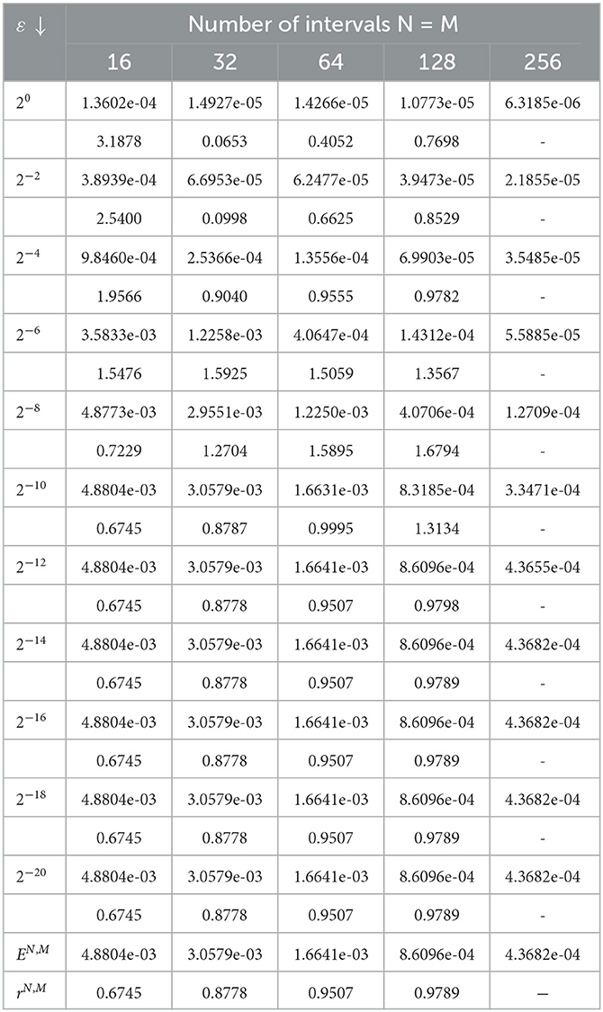
Table 2. $E_{\epsilon }^{N,M},E^{N,M},r_{\epsilon }^{N,M}$, and r^N,M for Example 4.2.

In Figures 1, 2, the numerical solutions of the method for Examples 4.1 and 4.2 for different values of ε are given, respectively, for N = 80 and M = 40. Figure 3 displays the effect ε on the solutions profile of the developed scheme for Examples 4.1 and 4.2. From the figures, we see that a strong boundary layer is created on the right side of the spatial domain as ε close to zero. Furthermore, in Figure 4, the maximum point wise errors of the scheme is shown by the log-log scale plot. From these figures, one can observe that maximum absolute error decreases as the step sizes decrease for every values of ε, which confirm ε-uniform convergence of the proposed scheme.

FIGURE 1

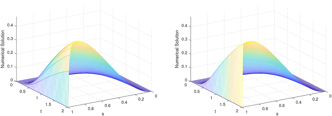
Figure 1. Numerical solution of Example 4.1 for ε = 2⁻⁶ and ε = 2⁻²⁰, respectively.

FIGURE 2

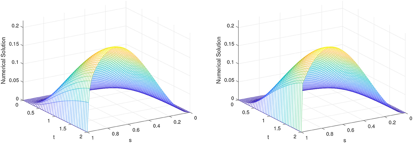
Figure 2. Numerical solution of Example 4.2 for ε = 2⁻⁶ and ε = 2⁻²⁰, respectively.

FIGURE 3

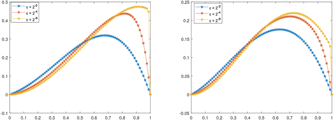
Figure 3. Effect of ε on solution profiles for Examples 4.1 and 4.2, respectively.

FIGURE 4

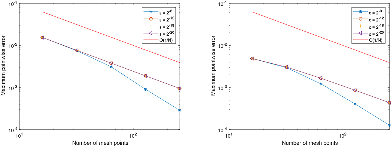
Figure 4. Maximum point wise error in log-log scale plot for Examples 4.1 and 4.2, respectively.

In Table 3, the comparison with results of the developed method with the existing recently published studies of [23, 29] are given for Example 4.1. In Table 4, the comparison with results of the developed method with the existing number of recently published studies of [15, 24, 29, 30] are given for Example 4.2. As one follows, the developed scheme holds more accurate.

TABLE 3

Table 3. E^N,M and r^N,M for Example 4.1.

TABLE 4

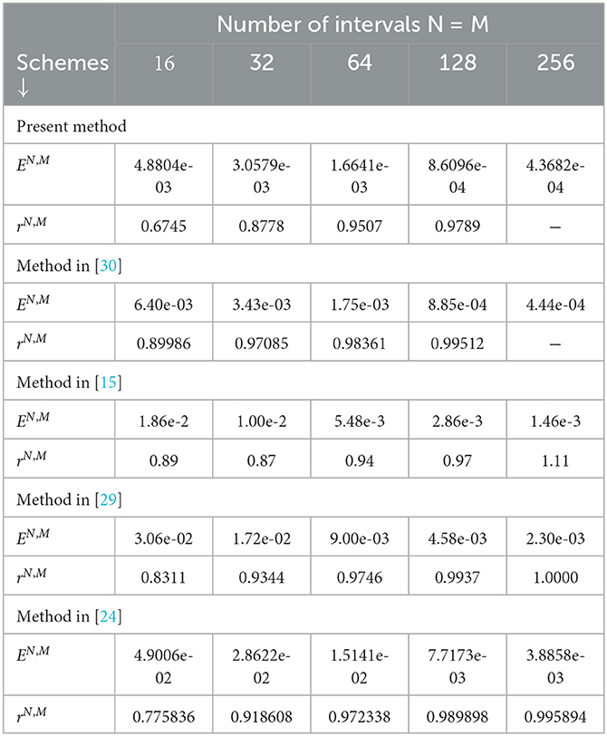
Table 4. E^N,M and r^N,M for Example 4.2.

5. Conclusion

We have developed a numerical method for solving singularly perturbed parabolic convection-diffusion equation with a large time delay. The solution of the problem exhibits a boundary layer on the right side of the domain. The solution has a steep gradient in the layer region due to the presence of ε. In the rapidly changing behavior of the solution in the layer region, one encounters computational difficulties to find the solution using analytically or using classical numerical methods. To handle this effect, we developed method comprises of the backward Euler scheme in the time direction and an exponentially fitted higher order finite difference scheme in the spatial direction. Using comparison principle, the stability of the discrete scheme is analyzed. The stability and uniformly convergent of the method are discussed theoretically. Numerical results are delineated by applying maximum point wise error, ε-uniform error and ε-uniform rate of convergence in tables which are in acceptable agreement with the theoretical analysis. The developed method contributes more accurate, stable, and ε-uniform with a linear order of convergence in the spatial and in the time direction. The proposed scheme can be extended for singularly perturbed turning point problems.

Data availability statement

The original contributions presented in the study are included in the article/supplementary material, further inquiries can be directed to the corresponding author.

Author contributions

ST and MW carried out the scheme development, algorithms writing, MATLAB code writing, the numerical simulations, and write final version of the manuscript. GD and TD planned the problem, design, wrote draft of the manuscript, and revised the manuscript. All authors read, commented, and approved the submitted version of the manuscript.

Acknowledgments

The authors would like to thank the referees for their constructive comments that improved the quality of this article.

Conflict of interest

The authors declare that the research was conducted in the absence of any commercial or financial relationships that could be construed as a potential conflict of interest.

Publisher's note

All claims expressed in this article are solely those of the authors and do not necessarily represent those of their affiliated organizations, or those of the publisher, the editors and the reviewers. Any product that may be evaluated in this article, or claim that may be made by its manufacturer, is not guaranteed or endorsed by the publisher.

References

1. Baker CT, Bocharov GA, Rihan FA. A Report on the Use of Delay Differential Equations in Numerical Modelling in the Biosciences. Citeseer (1999).

Google Scholar

2. Gopalsamy K. Stability and Oscillations in Delay Differential Equations of Population Dynamics. vol. 74. Springer Science and Business Media (1992).

Google Scholar

3. Bestehorn M, Grigorieva EV. Formation and propagation of localized states in extended systems. Ann Phys. (2004) 516:423–31. doi: 10.1002/andp.200451607-806

PubMed Abstract | CrossRef Full Text | Google Scholar

4. Govindarao L, Mohapatra J, Das A. A fourth-order numerical scheme for singularly perturbed delay parabolic problem arising in population dynamics. J Appl Math Comput. (2020) 63:171–95. doi: 10.1007/s12190-019-01313-7

CrossRef Full Text | Google Scholar

5. Tian H. Numerical Treatment of Singularly Perturbed Delay Differential Equations. Manchester, UK: The University of Manchester (2000).

PubMed Abstract | Google Scholar

6. Ansari AR, Bakr SA, Shishkin GI. A parameter-robust finite difference method for singularly perturbed delay parabolic partial differential equations. J Comput and Appl Math. (2007) 205:552–66. doi: 10.1016/j.cam.2006.05.032

CrossRef Full Text | Google Scholar

7. Das A, Natesan S. Uniformly convergent hybrid numerical scheme for singularly perturbed delay parabolic convection–diffusion problems on Shishkin mesh. Appl Math Comput. (2015) 271:168–86. doi: 10.1016/j.amc.2015.08.137

CrossRef Full Text | Google Scholar

8. Gowrisankar S, Natesan S. A robust numerical scheme for singularly perturbed delay parabolic initial-boundary-value problems on equidistributed grids. Electron Trans Numer Anal. (2014) 41:376–95. doi: 10.1016/j.cpc.2014.04.004

CrossRef Full Text | Google Scholar

9. Gupta V, Kumar M, Kumar S. Higher order numerical approximation for time dependent singularly perturbed differential-difference convection-diffusion equations. Num Methods Partial Differ Equ. (2018) 34:357–80. doi: 10.1002/num.22203

CrossRef Full Text | Google Scholar

10. Sumit, Kumar S, Kuldeep, Kumar M. A robust numerical method for a two-parameter singularly perturbed time delay parabolic problem. Comput Appl Math. (2020) 39:1–25. doi: 10.1007/s40314-020-01236-1

CrossRef Full Text | Google Scholar

11. Kumar S, Kumar M. High order parameter-uniform discretization for singularly perturbed parabolic partial differential equations with time delay. Comput Math Appl. (2014) 68:1355–67. doi: 10.1016/j.camwa.2014.09.004

CrossRef Full Text | Google Scholar

12. Gowrisankar S, Natesan S. ε-Uniformly convergent numerical scheme for singularly perturbed delay parabolic partial differential equations. Int J Comput Math. (2017) 94:902–21. doi: 10.1080/00207160.2016.1154948

CrossRef Full Text | Google Scholar

13. Das A, Natesan S. Second-order uniformly convergent numerical method for singularly perturbed delay parabolic partial differential equations. Int J Comput Math. (2018) 95:490–510. doi: 10.1080/00207160.2017.1290439

CrossRef Full Text | Google Scholar

14. Govindarao L, Mohapatra J. A second order numerical method for singularly perturbed delay parabolic partial differential equation. Eng Comput. (2018) 36:420–44. doi: 10.1108/EC-08-2018-0337

CrossRef Full Text | Google Scholar

15. Kumar D, Kumari P. A parameter-uniform scheme for singularly perturbed partial differential equations with a time lag. Num Methods Partial Differ Equ. (2020) 36:868–86. doi: 10.1002/num.22455

CrossRef Full Text | Google Scholar

16. Singh J, Kumar S, Kumar M. A domain decomposition method for solving singularly perturbed parabolic reaction-diffusion problems with time delay. Num Methods Partial Differ Equ. (2018) 34:1849–66. doi: 10.1002/num.22256

CrossRef Full Text | Google Scholar

17. Rao SCS, Kumar S. An almost fourth order uniformly convergent domain decomposition method for a coupled system of singularly perturbed reaction–diffusion equations. J Comput Appl Math. (2011) 235:3342–54. doi: 10.1016/j.cam.2011.01.047

CrossRef Full Text | Google Scholar

18. Kumar S, Kumar M. A second order uniformly convergent numerical scheme for parameterized singularly perturbed delay differential problems. Num Algor. (2017) 76:349–60. doi: 10.1007/s11075-016-0258-9

CrossRef Full Text | Google Scholar

19. Kumar S, Kumar M. Analysis of some numerical methods on layer adapted meshes for singularly perturbed quasilinear systems. Num Algor. (2016) 71:139–50. doi: 10.1007/s11075-015-9989-2

CrossRef Full Text | Google Scholar

20. Podila PC, Kumar K. A new stable finite difference scheme and its convergence for time-delayed singularly perturbed parabolic PDEs. Comput Appl Math. (2020) 39:1–16.

Google Scholar

21. Tesfaye SK, Woldaregay MM, Dinka TG, Duressa GF. Fitted computational method for solving singularly perturbed small time lag problem. BMC Res Notes. (2022) 15:318. doi: 10.1186/s13104-022-06202-0

PubMed Abstract | CrossRef Full Text | Google Scholar

22. Woldaregay MM, Aniley WT, Duressa GF. Novel numerical scheme for singularly perturbed time delay convection-diffusion equation. Adv Math Phys. (2021) 2021:6641236. doi: 10.1155/2021/6641236

CrossRef Full Text | Google Scholar

23. Negero NT, Duressa GF. An efficient numerical approach for singularly perturbed parabolic convection-diffusion problems with large time-lag. J Math Model. (2022) 10:173–90. doi: 10.22124/jmm.2021.19608.1682

CrossRef Full Text | Google Scholar

24. Babu G, Bansal K. A high order robust numerical scheme for singularly perturbed delay parabolic convection diffusion problems. J Appl Math Comput. (2021) 68:363–89. doi: 10.1007/s12190-021-01512-1

CrossRef Full Text | Google Scholar

25. Salama AA, Al-Amery DG. A higher order uniformly convergent method for singularly perturbed delay parabolic partial differential equations. Int J Comput Math. (2017) 94:2520–46. doi: 10.1080/00207160.2017.1284317

CrossRef Full Text | Google Scholar

26. Negero NT, Duressa GF. A method of line with improved accuracy for singularly perturbed parabolic convection–diffusion problems with large temporal lag. Results Appl Math. (2021) 11:100174. doi: 10.1016/j.rinam.2021.100174

CrossRef Full Text | Google Scholar

27. Sahoo SK, Gupta V. Parameter robust higher-order finite difference method for convection-diffusion problem with time delay. Num Methods Partial Differ Equ. (in press). doi: 10.1002/num.23039

CrossRef Full Text | Google Scholar

28. Rao SCS, Kumar S. Second order global uniformly convergent numerical method for a coupled system of singularly perturbed initial value problems. Appl Math Comput. (2012) 219:3740–53. doi: 10.1016/j.amc.2012.09.075

CrossRef Full Text | Google Scholar

29. Kumar D, Kumari P. A parameter-uniform numerical scheme for the parabolic singularly perturbed initial boundary value problems with large time delay. J Appl Math Comput. (2019) 59:179–206. doi: 10.1007/s12190-018-1174-z

CrossRef Full Text | Google Scholar

30. Negero NT, Duressa GF. Uniform convergent solution of singularly perturbed parabolic differential equations with general temporal-lag. Iran J Sci Technol Trans A Sci. (2022) 46:507–24. doi: 10.1007/s40995-021-01258-2

CrossRef Full Text | Google Scholar

31. Protter M, Weinberger H. Maximum Principles in Differential Equations. Englewood Cliffs, NJ: Prentice-Hall Inc. (1967).

Google Scholar

32. Kellogg RB, Tsan A. Analysis of some difference approximations for a singular perturbation problem without turning points. Math Comp. (1978) 32:1025–39.

Google Scholar

33. O'Malley RE. Singular Perturbation Methods for Ordinary Differential Equations. vol. 89. New York, NY: Springer (1991).

PubMed Abstract | Google Scholar