Role of the whitefly maturation period on mosaic disease propagation in Jatropha curcas plant

Mosaic disease in Jatropha curcas plants is caused by begomoviruses carried by whitefly vectors, and only mature vectors can transmit the virus. In this study, a mathematical model is developed for the dynamic analysis of the spread of mosaic disease in the J. curcas plantation, accounting for the whitefly maturation period as a time delay factor. The existence conditions and stability of the equilibrium points have been studied with qualitative theory. The basic reproduction number, R₀, is determined to study the stability of the disease-free equilibrium with respect to it. Transcritical bifurcation of the disease-free equilibrium and Hopf bifurcation of the endemic equilibrium are also analyzed. Using numerical simulations, the analytical findings are verified and discussed the different dynamical behaviors of the system. In this research, the stabilizing role of maturation delay has been established. That means when maturation time is large, disease will be transmitted when the infection rate is high.

1. Introduction

Whiteflies can transmit mosaic viruses (Begomoviruses) when they feed on infected Jatropha plants [1]. The transmission of the virus can occur quickly, often within minutes of the whitefly feeding on the infected plant. However, it is worth noting that the ability of whiteflies to transmit the virus can also depend on factors such as the maturation period of the whitefly population and the length of time the matured whitefly feeds on the infected plant. The maturation time of whiteflies can vary depending on the temperature, humidity, and host plant availability. Generally, the maturation time of whiteflies ranges from 20 to 30 days, during which time they develop from eggs to larvae and then to pupae and finally to adults [2]. Once the whiteflies have matured into adults, they can begin feeding on plants and transmitting Begomoviruses similar to a mosaic virus [3].

Jatropha curcas is a multi-purpose, drought-resistant tropical plant of the Euphorbiaceae family that can be grown in low-to-high rainfall areas [4]. This plant is affected by parasites and diseases, such as the mosaic disease caused by viruses of the Begomovirus family [5]. This disease manifests in substantial leaf damage, such as yellowing of the leaves and sap drainage, and it attacks the fruits, thus significantly reducing the yield of seeds. Whitefly (Bemisia tabaci) is the vector that carries the virus and transmits it to Jatropha plants, so the spread of the mosaic disease is primarily determined by the distribution of whitefly vectors and the density of the host plants [6, 7].

The viral infection of a plant is often considered a delayed process, which represents various processes associated with the production of virus particles by the vectors, vector maturation time, duration of feeding on the plants, entry of the virus into plant cells, etc. [8]. When considering plant disease, it is problematic from a practical point of view to distinguish between different stages of the plant infectious status; thus, identifying appropriate time delay from observing plant pathology status is a challenging problem [8–10].

From a mathematical perspective, delays in the disease transmission and development of symptoms can be effectively modeled using the formalism of delay differential equations (DDEs) [11, 12]. Several mathematical models have looked at the dynamics of plant diseases, starting with a seminal work of Van der Plank [13], who looked at the possibility of predicting whether an epidemic outbreak can occur and its size. Jeger et al. [14] provided a detailed review of recent study examining various interactions between plants and disease-carrying vectors. Jackson and Chen-Charpentier [15, 16] have recently studied the propagation of plant viruses while accounting for two-time delays, one representing the incubation period of the plant and the other being a shorter delay due to the incubation period of the vector. Time-delayed models have also proved effective for the analysis of within-plant dynamics of the immune response to viral infections [17].

In the particular context of mosaic disease affecting the population of J. curcas plant, several models have been proposed that have looked at the dynamics of control of and disease [18, 19]. Venturino et al. [19] have presented a mathematical model for the dynamics of J. curcas plant's mosaic disease though they focused on a constant disease transmission rate. In [20], authors have looked at the effects of roguing delay, which caused stable oscillations in plants and vector populations. These earlier models of plant mosaic disease have assumed a constant disease transmission, without account for vector maturation time [9]. Matured vector can only fids on plants biomass, and the maturation time of vector whitefly is 20–30 days depending on temperature and other weather conditions [2, 19]. To make the model more realistic, an epidemic model for the mosaic disease is proposed here that explicitly accounts for whitefly maturating time as a delayed process in this study.

Basic reproductive number (R₀) plays an important role in understanding the dynamics of a plant disease. It is the expected number of susceptible individuals that an infected individual can infect []. The stability of the disease-free equilibrium can be studied using the range of the basic reproductive number. Disease-free equilibrium is stable when R₀ is below unity, and system becomes endemic when R₀ crosses unity. In this research, basic reproduction number, R₀ is derived to study the stability of the disease-free equilibrium using R₀ and also to analyse the forward bifurcation.

The outline of the article is as follows. In the next section, a time-delayed model of mosaic disease transmission has been formulated and discussed the main properties of the model in Section 3. The Section 4 is devoted to analyzing the feasibility and stability of different steady states of the model. In Section 5, numerical techniques are used to perform and illustrate the model's behavior in different dynamical regimes. The article concludes in Section 6 with a discussion of results and future outlook.

2. Formulation of the mathematical model

In this section, the delay model is derived for mosaic disease transmission in J. curcas plantation. The following hypotheses are taken in formulating the desired mathematical model.

– Let S(t) and I(t) be the susceptible and infected plant populations, respectively, while non-infective and infective whitefly populations are denoted by U(t) and V(t). Vector population is considered in the modeling process without explicitly considering a separate compartment for the mosaic virus (begomovirus).

– Due to the finite area of a plantation, a logistic growth is assumed for susceptible plants, with the intrinsic growth rate r and the carrying capacity K.

– Susceptible plant becomes infected, while an infected vector feeds on a healthy plant leaf or stem. Similarly, a non-infected vector becomes infected upon feeding on an infected portion of the plant [21, 22].

– Infected vectors transmit the disease to susceptible plant at a rate λ, while uninfected vectors themselves pick up the disease from the infected plants at rate β.

– For the dynamics of vector population, b is considered to be the net growth rate of non-infective vectors and a to be the maximum number of vectors that can survive on a plant. Then, a(S + I) > 0 is the overall carrying capacity of the vectors on all plant biomass, m is taken as the removal rate of infected plant biomass, and μ is the natural mortality rate of the infected vectors.

– The maturation time of the vector is assumed as a time delay factor. Thus, infection transmission in a Jatropha plant by whitefly vector is a delayed process. In order to model this mathematically, the transmission of infection is expressed at time t by the term λe ^{− mτ}SV(t − τ), where m and λ are positive constants. The term e ^{− mτ} represents the survival probability of inoculum through the maturation time [t − τ, t].

From the assumptions made above, the following mathematical model can be formulated:

$\begin{array}{ll}\begin{array}{c}\frac{dS}{dt}=rS\left[1-\frac{S+I}{K}\right]-\lambda e^{-m\tau }SV(t-\tau ),\hfill \\ \frac{dI}{dt}=\lambda e^{-m\tau }SV(t-\tau )-mI,\hfill \\ \frac{dU}{dt}=bU\left[1-\frac{U+V}{a(S+I)}\right]-\beta UI,\hfill \\ \frac{dV}{dt}=\beta UI-\mu V.\hfill \end{array}& (1)\end{array}$

For biological reasons, the plant and vector populations cannot have negative values; hence, the initial function for model (1) is taken as follows:

$\begin{array}{ll}\begin{array}{c}S(\gamma )={\varphi }_1(\gamma ),I(\gamma )={\varphi }_2(\gamma ),U(\gamma )={\varphi }_3(\gamma ),V(\gamma )={\varphi }_4(\gamma ),\hfill \\ {\varphi }_i(\gamma )\ge 0,\gamma \in \left[-\tau ,0\right],{\varphi }_i(0)>0,i=1,2,3,4.\hfill \end{array}& (2)\end{array}$

Using the result established in [12, 23], it can be shown that the solution [S(t), I(t), U(t), V(t)]^T of the model (1) with the initial condition (2) exists and is unique on [0, +∞].

Before proceeding with the main analysis of the model (1), the basic properties of the model are discussed in the next section.

3. Basic properties of the model (1)

In this section, the basic properties of the delay model (1) such as non-negativity, boundedness of solutions, basic reproduction number, etc. are analyzed.

3.1. Non-negativity

The following theorem is derived for the non-negativity of solutions.

Theorem 1. All solutions of model (1) with the initial condition (2) remain non-negative for t ≥ 0.

Proof. I rewrite the first equation of (1) as

$\begin{array}{ll}\frac{dS}{dt}-S\left[r\left(1-\frac{S+I}{k}\right)-\lambda e^{-m\tau }V(t-\tau )\right]=0.& (3)\end{array}$

Let $f(S,I,V)=r(1-\frac{S+I}{k})-\lambda e^{-m\tau }V(t-\tau )$, then from the above equation, one can get

$\begin{array}{l}\frac{dS}{dt}-Sf(S,I,V)=0,\\ \Rightarrow \left[\frac{dS}{dt}-Sf(S,I,V)\right]e^{-{\int }_0^{t}f(\theta )d\theta }=0,\\ \Rightarrow \frac{d}{dt}\left[S{e}^{-{\int }_0^{t}f(\theta )d\theta }\right]=0.\end{array}$

Since S(0) = ϕ₁(γ) > 0, then S(t) > 0 for t ≥ 0.

An identical argument can establish the non-negativity of U(t). To prove the result for I(t) and V(t), let t₁ > 0 be the first time when I(t₁)V(t₁) = 0, and let us assume that at this point I(t₁) = 0 and V(t₁) ≥ 0. The second equation of model (1) then shows that at t = t₁, one has

$\frac{dI(t_1)}{dt}=\lambda e^{-m\tau }S(t_1)V(t_1-\tau )-mI(t_1)=\lambda e^{-m\tau }S(t_1)V(t_1-\tau )\ge 0,$

implying that I(t) ≥ 0 for all t ≥ 0. Now that the non-negativity of I(t) has been established, if there is ever t₂ > 0 such that V(t₂) = 0, at this moment one would also have

$\frac{dV(t_2)}{dt}=\beta U(t_2)I(t_2)-\mu V(t_2)=\beta U(t_2)I(t_2)\ge 0,$

which again proves that V(t) ≥ 0 for t ≥ 0.     □

3.2. Boundedness

To ensure the model remains biologically plausible, plant and vector populations must remain bounded during their time evolution. Let us denote by M(t) the total plant biomass, i.e., M(t) = S(t)+I(t), then it satisfies the equation

$\frac{dM}{dt}=rS\left[1-\frac{S+I}{K}\right]-mI\le rM\left(1-\frac{M}{K}\right),\Rightarrow$

${\displaystyle \underset{t\to \infty }{lim sup}}M(t)\le B,$

where B = max[M(0), K], and hence, the total plant biomass is bounded. Non-negativity of solutions implies that the third equation of model (1) can be rewritten as follows:

$\frac{dU}{dt}=bU\left[1-\frac{U}{a(S+I)}\right]-\mu UI\le bU\left[1-\frac{U}{a(S+I)}\right],\Rightarrow$

${\displaystyle \underset{t\to \infty }{lim sup}}U(t)\le aB.$

Similarly, from the last equation of (1), one obtains

$\frac{dV}{dt}=\beta UI-\mu V\le \beta a{B}^2-\mu V,\Rightarrow {\displaystyle \underset{t\to \infty }{lim sup}}V(t)\le \frac{\beta a{B}^2}{\mu }.$

From the above calculation, the following positively invariant set is obtained

$\begin{array}{l}\mathcal{D}=\{(S,I,U,V)\in {ℝ}_{+}^4:0\le S,I\le B,0\le U\le aB,\\ 0\le V\le \frac{\beta a{B}^2}{\mu }\},& (4)\end{array}$

which attracts each solution of the model (1) that starts within the set for a sufficiently large t > 0.

3.3. Basic reproduction number

The method used by Hefferman et al. [24] for calculating the basic reproduction number (R₀).

The next generation matrix G is a combination of two parts, namely, the matrix F (where F_i is the new infections) and the matrix V (where V_i transfers the infections from one compartment to another). The matrices are given as

$F=\left[\frac{\partial F_i(E_1)}{\partial x_j}\right]=\left[\begin{array}{cc}0& \lambda e^{-m\tau }K\\ 0& 0\end{array}\right]$

and

$V=\left[\frac{\partial V_i(E_1)}{\partial x_j}\right]=\left[\begin{array}{cc}m& 0\\ -\beta e^{-\mu }aK& \mu \end{array}\right].$

Here, indices i and j correspond to I and V, respectively, and E₂(K, 0, aK, 0) is the disease-free steady-state of the system.

According to [24], the basic reproduction number R₀ is taken as the dominant eigenvalue of the matrix G = FV⁻¹ and obtained as

$\begin{array}{ll}{R}_0=\frac{a{K}^2\beta \lambda }{m\mu e^{m\tau }}.& (5)\end{array}$

3.4. Characteristic equation

The characteristic equation for eigenvalues ρ of linearization near any steady point $E(\bar{S},Ī,Ū,\bar{V})$ has the form

$\begin{array}{ll}△(\rho )=\mid \rho I-A-e^{-\rho \tau }D\mid =0,& (6)\end{array}$

where the matrices A and D are given by

$A=\left[a_{ij}\right]=\left(\begin{array}{cccc}{a}_{11}& a_{12}& 0& 0\\ \\ a_{21}& a_{22}& 0& 0\\ \\ a_{31}& a_{32}& a_{33}& a_{34}\\ \\ 0& a_{42}& a_{43}& a_{44}\end{array}\right)$

and

$D=\left[d_{ij}\right]=\left(\begin{array}{cccc}0& 0& 0& d_{14}\\ 0& 0& 0& d_{24}\\ 0& 0& 0& 0\\ 0& 0& 0& 0\end{array}\right),$

with

$\begin{array}{l}{a}_{11}=r\left[1-\frac{2\overline{S}+\overline{I}}{K}\right]-\lambda e^{-m\tau }\overline{V},\hfill \\ a_{12}=-\frac{r\overline{S}}{K},a_{21}=\lambda e^{-m\tau }\overline{V},a_{22}=-m,\hfill \\ a_{31}=\frac{b\overline{U}(\overline{U}+\overline{V})}{a{(\overline{S}+\overline{I})}^2}, a_{32}=-\beta \overline{U}+\frac{b\overline{U}(\overline{U}+\overline{V})}{a{(\overline{S}+\overline{I})}^2},\hfill \\ a_{33}=b[1-\frac{2\overline{U}+\overline{V})}{a(\overline{S}+\overline{I})}]-\beta \overline{I},\hfill \\ a_{34}=-\frac{b\overline{U}}{a(\overline{S}+\overline{I})},a_{42}=\beta \overline{U},a_{43}=\beta \overline{I},a_{44}=-\mu ,\hfill \end{array}$

and

$d_{14}=-\lambda e^{-m\tau }\bar{S},d_{24}=\lambda e^{-m\tau }\bar{S}.$

The characteristic equation (6) has the explicit form

$\begin{array}{l}\varphi (\rho ,\tau )={\rho }^4+J_1{\rho }^3+J_2{\rho }^2+J_3\rho +J_4+e^{-\rho \tau }\end{array}$

$\begin{array}{ll}(B_1{\rho }^2+B_2\rho +B_3)=0,& (7)\end{array}$

where the coefficients are given below,

$\begin{array}{l}{J}_1=-[a_{11}+a_{22}+a_{33}+a_{44}],B_1=-d_{14}{a}_{42},\hfill \\ J_2=(a_{11}+a_{22})(a_{33}+a_{44})+a_{11}{a}_{22}-a_{12}{a}_{21}\hfill \\ -a_{34}{a}_{43}+a_{33}{a}_{44},\hfill \\ J_3=(a_{11}+a_{22})(a_{34}{a}_{43}-a_{33}{a}_{44})+(a_{33}+a_{44})\hfill \\ (a_{12}{a}_{21}-a_{11}{a}_{22}),\hfill \\ J_4=(a_{12}{a}_{21}-a_{11}{a}_{22})(a_{34}{a}_{43}-a_{33}{a}_{44}),\hfill \\ B_2=d_{14}{a}_{42}(a_{33}-a_{11}-a_{21}-a_{42}),\hfill \\ B_3=d_{14}\{a_{33}{a}_{42}(a_{21}-a_{11})+a_{43}[(a_{11}+a_{21})\hfill \\ (a_{42}-a_{31})+a_{31}(a_{12}+a_{22})]\}.\hfill \end{array}$

4. Steady states and their stability

The system (1) has up to three possible equilibria, namely,

(a) the axial equilibrium, E₁ = (K, 0, 0, 0)

(b) the disease-free equilibrium (DFE), E₂ = (K, 0, aK, 0)

(c) the endemic equilibrium point (EEP), E^* = (S^*, I^*, U^*, V^*)

where

$I^{*}=\frac{r{S}^{*}(K-S^{*})}{r{S}^{*}+Km},U^{*}=\frac{m\mu }{\beta \lambda e^{-m\tau }{S}^{*}},$

$V^{*}=\frac{rm(K-S^{*})}{(r{S}^{*}+mK)\lambda e^{-m\tau }},$

and S^* satisfies the quartic equation

$\begin{array}{ll}F(S^{*})=l_0{S}^4+l_1{S}^3+l_2{S}^2+l_{3}S+l_4=0& (8)\end{array}$

where,

$\begin{array}{l}{l}_0=a{\beta }^{2}Kr(r+m)\lambda e^{-m\tau }>0,\\ l_1=arK(r+m)\left[b-\beta K\right]\lambda e^{-m\tau }+bm\beta r^2,\\ l_2=a{K}^2(r+m)bm\lambda e^{-m\tau }-bm{r}^2\mu -\beta bmrK(r-m),\\ l_3=-b{m}^{2}rK\left[2\mu +K\beta \right]<0,\\ l_4=-b{m}^3\mu r{K}^2<0.\end{array}$

To ensure biological feasibility of E^*, i.e., positivity of all state variables, one has to require S^* < K.

Since F(0) < 0 and $\underset{x\to \infty }{lim}F(x)=\infty$, Equation (8) always has at least one positive root. Using the Descartes's rule of signs, one can state the following result.

Theorem 2. Let

$\begin{array}{l}d=256l_0^3{l}_4^3-192l_0^2{l}_1{l}_3{l}_4^2-128l_0^2{l}_2^2{l}_4^2+144l_0^2{l}_2{l}_3^2{l}_4-27l_0^2{l}_3^4\\ +144l_0{l}_1^2{l}_2{l}_4^2-6l_0{l}_1^2{l}_3^2{l}_4-80l_0{l}_1{l}_2^2{l}_3{l}_4+18l_0{l}_1{l}_2{l}_3^3+16l_0{l}_2^4{l}_4\\ -4l_0{l}_2^3{l}_3^2-27l_1^4{l}_4^2+18l_1^3{l}_2{l}_3{l}_4-4l_1^3{l}_3^3-4l_1^2{l}_2^3{l}_4+l_1^2{l}_2^2{l}_3^2\end{array}$

be the discriminant of Equation (8). If d > 0, and either l₁ > 0, or l₂ < 0, then Equation (8) has a single positive root. If d ≥ 0, and l₁ < 0, or l₂ > 0, the Equation (8) has three positive roots, with one double root if d = 0.

Since b − βK > 0 implies l₁ > 0, the following proposition is proposed.

Proposition 3. Suppose d > 0, b > βK, and S^* < K, then model (1) has unique co-existence steady state.

The steady state E₁ is unstable for any parameter values as one of its characteristic eigenvalues is equal to b > 0.

4.1. Stability of DFE

At the disease-free steady state E₂, two eigenvalues of the characteristic equation are −b and −r, and the remaining roots satisfy the transcendental equation

$\begin{array}{ll}H(\rho )={\rho }^2+(m+\mu )\rho +m\mu -e^{-(m+\rho )\tau }a{K}^2\beta \lambda =0.& (9)\end{array}$

The following theorem is established concerning the stability of the steady state E₂.

Theorem 4. (i) For R₀ < 1, the disease-free equilibrium E₂ of the model (1) is asymptotically stable

(ii) For R₀ = 1, E₂ is linearly neutrally stable

(iii) For R₀ > 1, E₂ is unstable.

Proof. (i) let us assume R₀ < 1, which implies aK²βλe^−mτ < mμ, i.e., M₃ < M₂. We note that in this case for τ = 0 that all characteristic roots of Equation (9) have negative real part, and, therefore, our goal is to show that as τ > 0, none of the characteristic roots can reach the imaginary axis. Let us assume by contradiction that for some τ > 0, ρ = iκ is a root of (9). Substituting this into (12) yields

$\begin{array}{ll}{\kappa }^4+{\kappa }^2(m^2+{\mu }^2)+(M_2^2-M_3^2)=0.& (10)\end{array}$

Since this equation has no positive real roots for κ, it means that the characteristic equation (9) cannot have purely imaginary roots, and hence, R₀ < 1 the steady state E₂ is linearly asymptotically stable for all τ ≥ 0.

(ii) If R₀ = 1, then ρ = 0 is a simple characteristic root of (9). Let ρ = η+iκ by any other characteristic root, then the Equation (9) turns into

$\begin{array}{ll}{(\eta +i\kappa )}^2+(\eta +i\kappa )M_1+M_2=e^{-(\eta +i\kappa )\tau }{M}_3,& (11)\end{array}$

with M₁ = m + μ, M₂ = mμ, and $M_3=a{K}^2\beta \lambda e^{-m\tau }$.

By separating the real and imaginary parts, one can obtain

$\begin{array}{c}-{\kappa }^2+{\eta }^2+\eta M_1+M_2=e^{-\eta \tau }{M}_{2}cos\kappa \tau ,\hfill \\ 2\eta \kappa +\kappa M_1=e^{-\eta \tau }{M}_{2}sin\kappa \tau ,\hfill \end{array}$

First squaring and then adding the two equations, the following equation is derived

$\begin{array}{l}{({\eta }^2+{\kappa }^2)}^2+{\kappa }^2(m^2+{\mu }^2)+(\eta M_1+M_2^2)\end{array}$

$\begin{array}{ll}+2\eta ({\kappa }^2{M}_1+\eta M_2)=e^{-2\eta \tau }{M}_2^2.& (12)\end{array}$

The relation in (12) is true only for η < 0. Thus, for R₀ = 1, the disease-free equilibrium point E₂ is linearly neutrally stable.

For R₀ > 1, $H(0)=m\mu -e^{-m\tau }a{K}^2,\beta \lambda =m\mu (1-R_0)<0$, and since $\underset{\rho \to \infty }{lim}H(\rho )=\infty$, there exists at least one positive root of the Equation (9), implying that for R₀ > 1, E₂ is unstable.     □

4.2. Stability of EEP

At the endemic equilibrium E^*, the coefficients of the characteristic equation (7) depend on the time delay τ, which makes it impossible to derive closed form conditions for stability switches. To gain some understanding of how the stability of E^* depends on parameters, we first consider the case where the maturation time of vectors is very small, so that one can assume τ = 0.

4.2.1. Stability analysis without delay

In this case, the characteristic equation (7) transforms into a quartic equation

$\begin{array}{ll}{\rho }^4+{\alpha }_1{\rho }^3+{\alpha }_2{\rho }^2+{\alpha }_3\rho +{\alpha }_4=0,& (13)\end{array}$

where α_i, i = 1, 2, 3, 4 are given below:

$\begin{array}{c}{\alpha }_1=-(m_{11}+m_{22}+m_{33}+m_{44}),\hfill \\ {\alpha }_2=-m_{12}{m}_{21}+m_{11}(m_{22}+m_{33}+m_{44})\hfill \\ +m_{22}(m_{33}+m_{44})-m_{14}{m}_{42}\hfill \\ -m_{34}{m}_{43}+m_{33}{m}_{44},\hfill \\ {\alpha }_3=(m_{11}+m_{22})(m_{34}{m}_{43}-m_{33}{m}_{44})\hfill \\ +(m_{33}+m_{44})(m_{12}{m}_{21}-m_{11}{m}_{22})\hfill \\ -m_{14}{m}_{42}(m_{11}+m_{21}+m_{33}+m_{43}),\hfill \\ {\alpha }_4=m_{14}(m_{11}+m_{21})(m_{33}{m}_{42}-m_{31}{m}_{43}+m_{42}{m}_{43})\hfill \\ +m_{14}{m}_{31}{m}_{43}(m_{12}+m_{12})\hfill \\ +(m_{33}{m}_{44}-m_{34}{m}_{43})(m_{11}{m}_{22}-m_{12}{m}_{21}),\hfill \end{array}$

and

$\begin{array}{c}{m}_{11}=m_{12}=-\frac{r{S}^{*}}{K},m_{21}=\lambda V^{*},m_{22}=-m,\hfill \\ m_{14}=-m_{24}=-\lambda S^{*},\hfill \\ m_{31}=\frac{b{U}^{*}(U^{*}+V^{*})}{a{(S^{*}+I^{*})}^2},m_{42}=\beta U^{*},m_{32}=m_{31}-m_{42},\hfill \\ m_{33}=-\frac{b{U}^{*}}{a(S^{*}+I^{*})},m_{34}=-\frac{b{U}^{*}}{a(S^{*}+I^{*})},\hfill \\ m_{44}=-\mu ,m_{43}=\beta I^{*}.\hfill \end{array}$

Since α₁ > 0 for all parameter values, in light of Routh-Hurwitz criterion [25], the characteristic equation (13) has roots with negative real parts if

$\begin{array}{l}{\alpha }_2>0,{\alpha }_3>0,{\alpha }_4>0,{\alpha }_1{\alpha }_2-{\alpha }_3>0,\text{ and}\\ ({\alpha }_1{\alpha }_2-{\alpha }_3){\alpha }_3-{\alpha }_1^2{\alpha }_4>0.\end{array}$

Thus, we have the following result.

Theorem 5. For τ = 0, the endemic equilibrium point E^* of the system (1) is asymptotically stable if the conditions given below are fulfilled:

$\begin{array}{l}{\alpha }_2>0,{\alpha }_3>0,{\alpha }_4>0,{\alpha }_1{\alpha }_2-{\alpha }_3>0,\text{ and}\end{array}$

$\begin{array}{ll}({\alpha }_1{\alpha }_2-{\alpha }_3){\alpha }_3-{\alpha }_1^2{\alpha }_4>0.& (14)\end{array}$

Now that the conditions for stability of the endemic steady state E^* have been established, the next question is whether stability can change depending on system parameters. We focus on the disease transmission rate λ, which is one of the biologically most important parameters representing an aggregate rate at which mosaic disease is passed from disease-carrying vectors to plants. Hopf bifurcation of the endemic steady state can occur if the characteristic equation (13) has a pair of purely imaginary eigenvalues for some λ = λ^* ∈ (0, ∞), with all other eigenvalues having negative real parts. For the Hopf bifurcation to actually take place, the transversality condition

$\frac{d\text{Re}\left[\rho (\lambda )\right]}{d\lambda }{|}_{{\lambda }^{*}}\ne 0$

should be satisfied.

Let us define a continuously differentiable function Φ : (0, ∞) → R of λ as follows:

$\Phi (\lambda ):={\alpha }_1(\lambda ){\alpha }_2(\lambda ){\alpha }_3(\lambda )-{\alpha }_3^2(\lambda )-{\alpha }_4(\lambda ){\alpha }_1^2(\lambda ).$

We then have the following result.

Theorem 6. The endemic equilibrium E^* of the system (1) with τ = 0 undergoes a Hopf bifurcation at λ = λ^* ∈ (0, ∞) if and only if

$\begin{array}{ll}\begin{array}{c}{\alpha }_2({\lambda }^{*})>0,{\alpha }_3({\lambda }^{*})>0,{\alpha }_4({\lambda }^{*})>0,\hfill \\ {\alpha }_1({\lambda }^{*}){\alpha }_2({\lambda }^{*})-{\alpha }_3({\lambda }^{*})>0,\hfill \\ \Phi ({\lambda }^{*})=0,\text{ and }{\alpha }_1^3{\alpha }_2^{\prime }{\alpha }_3({\alpha }_1-3{\alpha }_3)\hfill \\ \ne ({\alpha }_2{\alpha }_1^2-2{\alpha }_3^2)({\alpha }_3^{\prime }{\alpha }_1^2-{\alpha }_1^{\prime }{\alpha }_3^2).\hfill \end{array}\hfill & (15)\end{array}$

Moreover, at λ = λ^*, two characteristic eigenvalues ρ(λ) are purely imaginary, and the other two have negative real parts. Here, primes denote differentiation with respect to λ.

Proof. Using conditions (15), the characteristic equation (13) can be equivalently rewritten in the form

$\begin{array}{ll}\left({\rho }^2+\frac{{\alpha }_3}{{\alpha }_1}\right)\left({\rho }^2+{\alpha }_1\rho +\frac{{\alpha }_1{\alpha }_4}{{\alpha }_3}\right)=0.\hfill & (16)\end{array}$

Two roots of this equation are given by

${\rho }_{1,2}=\pm i{\omega }_0\text{ and\hspace{1em}}{\omega }_0=\sqrt{\frac{{\alpha }_3}{{\alpha }_1}},$

while the other two roots, ρ₃ and ρ₄ satisfy the equation

${\rho }^2+{\alpha }_1\rho +\frac{{\alpha }_1{\alpha }_4}{{\alpha }_3}=0,$

and from the Routh-Hurwitz criterion, they both have a negative real part.

To verify the transversality condition, we first note that Φ(λ^*) is a continuous function of its argument, and hence, there exists an open interval λ ∈ (λ^* − ϵ, λ^* + ϵ), where ρ₁ and ρ₂ are complex conjugate roots of the characteristic equation, which can be written in the general form as

$\begin{array}{l}{\rho }_{1,2}(\lambda )=\zeta (\lambda )\pm i\nu (\lambda ),\hfill \end{array}$

with ${\rho }_{1,2}({\lambda }^{*})=\pm i{\omega }_0$.

Substituting ρ_j(λ) = ζ(λ)±iν(λ) into the characteristic equation (13), differentiating with respect to λ, and separating real and imaginary parts gives

$\begin{array}{ll}P(\lambda ){\zeta }^{\prime }(\lambda )-Q(\lambda ){\nu }^{\prime }(\lambda )+R(\lambda )=0,& (17)\end{array}$

$\begin{array}{l}Q(\lambda ){\zeta }^{\prime }(\lambda )+P(\lambda ){\nu }^{\prime }(\lambda )+S(\lambda )=0,\end{array}$

where

$\begin{array}{l}P(\lambda )=4{\zeta }^3-12\zeta {\nu }^2+3{\alpha }_1({\zeta }^2-{\nu }^2)+2{\alpha }_2\zeta +{\alpha }_3,\\ Q(\lambda )=12{\zeta }^2\nu +6{\alpha }_1\zeta \nu -4{\zeta }^3+2{\alpha }_2\zeta ,\\ R(\lambda )={\alpha }_1{\zeta }^3-3{\alpha }_1^{\prime }\zeta {\nu }^2+{\alpha }_2^{\prime }({\zeta }^2-{\nu }^2)+{\alpha }_3^{\prime }\zeta ,\\ S(\lambda )=3{\alpha }_1^{\prime }{\zeta }^2\nu -{\alpha }_1^{\prime }{\nu }^3+2{\alpha }_2^{\prime }\zeta \nu +{\alpha }_3^{\prime }\zeta .\end{array}$

Solving the (17) for ζ′(λ^*) and using the condition (15) yields

$\begin{array}{l}{\left[\frac{d\text{Re}[{\rho }_j(\lambda )]}{d\lambda }\right]}_{\lambda ={\lambda }^{*}}={\zeta }^{\prime }({\lambda }^{*})=-\frac{Q({\lambda }^{*})S({\lambda }^{*})+P({\lambda }^{*})R({\lambda }^{*})}{P^2({\lambda }^{*})+Q^2({\lambda }^{*})}\\ =\frac{{\alpha }_1^3{\alpha }_2^{\prime }{\alpha }_3({\alpha }_1-3{\alpha }_3)-2({\alpha }_2{\alpha }_1^2-2{\alpha }_3^2)({\alpha }_3^{\prime }{\alpha }_1^2-{\alpha }_1^{\prime }{\alpha }_3^2)}{{\alpha }_1^4{({\alpha }_1-3{\alpha }_3)}^2+4{({\alpha }_2{\alpha }_1^2-2{\alpha }_3^2)}^2}\ne 0.\end{array}$

Thus, the transversality condition holds, and consequently, a Hopf bifurcation occurs at λ = λ^*.     □

4.2.2. Stability analysis with delay

To investigate whether increasing time delay τ can affect stability of the co-existence steady state E^*, we look at the characteristic equation (7) at the steady state E^*. Stability changes of E^* can only occur if the characteristic equation (7) has purely imaginary solutions.

In this case, the characteristic equation becomes

$\begin{array}{l}\varphi (\rho ,\tau )={\rho }^4+J_1{\rho }^3+J_2{\rho }^2+J_3\rho +J_4\end{array}$

$\begin{array}{ll}+e^{-\rho \tau }(B_1{\rho }^2+B_2\rho +B_3)=0,& (18)\end{array}$

Substituting ρ = iω into this equation and separating real and imaginary parts gives

$\begin{array}{ll}\begin{array}{c}{\omega }^4-J_2{\omega }^2+J_4=({\omega }^2{B}_1-B_3)cos\omega \tau -\omega B_{2}sin\omega \tau ,\hfill \\ J_1{\omega }^3-J_3\omega =({\omega }^2{B}_1-B_3)sin\omega \tau +\omega B_{2}cos\omega \tau .\hfill \end{array}& (19)\end{array}$

Squaring and adding these two equations yields the following equation for the Hopf frequency ω:

$\begin{array}{ll}{z}^4+{\delta }_1{z}^3+{\delta }_2{z}^2+{\delta }_{3}z+{\delta }_4=0,& (20)\end{array}$

where z = ω² and

$\begin{array}{c}{\delta }_1={J_1}^2-2J_2,{\delta }_2=2J_4+J_2^2-2J_1{J}_3-B_1^2,\text{ and}\\ {\delta }_3=-2J_4{J}_2+J_3^2+2B_1{B}_3-B_2^2,{\delta }_4=J_4^2-B_3^2.\end{array}$

Provided the Routh-Hurwitz criterion for Equation (20) holds, all of its roots will have a negative real part, and hence, there will be no purely imaginary roots of the characteristic equation (18). Thus, we have the following proposition.

Proposition 7. For τ = 0, the co-existence steady state E^* is linearly asymptotically stable for all τ ≥ 0 if the conditions of (14) hold and the following conditions are satisfied for all τ > 0:

$\begin{array}{ll}{\delta }_1>0,{\delta }_4>0,{\delta }_1{\delta }_2-{\delta }_3>0\text{and\hspace{1em}}({\delta }_1{\delta }_2-{\delta }_3){\delta }_3-{\delta }_1^2{\delta }_4>0.& (21)\end{array}$

Instead, if δ₄ < 0, Equation (20) possesses at least one real root z₀ > 0, and then ρ = ±iω₀ with ${\omega }_0=\sqrt{z_0}$ will be two roots of the characteristic equation (18).

From the system (19), one can determine the value of time delays at which this pair of purely imaginary roots occurs:

$\begin{array}{l}\hfill {\tau }^{*}=\frac{1}{{\omega }_0}{cos}^{-1}\\ \left[\frac{{\omega }_0^2{B}_3(J_1{\omega }_0^2-J_3)+(B_1{\omega }_0^2-B_3)({\omega }_0^4-J_2{\omega }_0^2+J_4)}{{(B_1{\omega }_0^2-B_3)}^2+B_2^2{\omega }_0^2}\right]\end{array}$

$\begin{array}{rr}\hfill +\frac{2\pi n}{{\omega }_0},n=0,1,2,3,...& (22)\end{array}$

Of course, δ₄ < 0 is just one possibility, where the characteristic equation (18) has a pair of purely complex eigenvalues, and this can also happen for δ₄ > 0, provided some of δ₁, δ₂, or δ₃ are sufficiently negative to ensure that Equation (20) has at least one real positive root. Whenever this happens, we have the following result.

Theorem 8. For τ = 0, the steady state E^* undergoes a Hopf bifurcation at τ = τ^*, provided the following condition holds

$\begin{array}{ll}4{\omega }_0^6+{\pi }_1{\omega }_0^4+{\pi }_2{\omega }_0^2+{\pi }_3\ne 0,& (23)\end{array}$

where

${\pi }_1=3J_1-6J_2,{\pi }_2=2J_2+4J_4-4J_1{J}_3-2B_1^2,\text{ and}$

${\pi }_3=J_3^2-2J_2{J}_4-B_2^2+2B_1{B}_3.$

Proof. In light of the above analysis, at τ = τ^*, the characteristic equation (18) has a pair of purely imaginary eigenvalues. Hence, to complete the proof of the theorem, it remains to prove the transversality condition, i.e., that the characteristic eigenvalues cross the imaginary axis. To this end, we differentiate characteristic equation (18) with respect to τ to obtain

$\begin{array}{l}\frac{d\tau }{d\rho }=\frac{4{\rho }^3+3(J_1{\rho }^2+2J_2\rho +J_3)}{B_1{\rho }^3+B_2{\rho }^2+B_3\rho }{e}^{\rho \tau }+\frac{2B_1\rho +B_2}{B_1{\rho }^3+B_2{\rho }^2+B_3\rho }-\frac{\tau }{\rho }.\end{array}$

Evaluating this at τ = τ^* and using relations (19), we find

$\text{sgn}{\left[\frac{dRe(\rho )}{d\tau }\right]}_{\tau ={\tau }^{*}}=\text{sgn}{\left[Re{\left(\frac{d\rho }{d\tau }\right)}^{-1}\right]}_{\rho =i{\omega }_0}$

$\text{sgn}\left[\frac{4{\omega }_0^6+{\pi }_1{\omega }_0^4+{\pi }_2{\omega }_0^2+{\pi }_3}{B_2{\omega }_0^2+{(-B_1{\omega }_0^2+B_3)}^2}\right].$

Since the denominator of this expression is always positive, if the condition of the theorem holds, this means that the transversality condition

$\text{sgn}{\left[\frac{dRe(\rho )}{d\tau }\right]}_{\tau ={\tau }^{*}}\ne 0$

is satisfied, and thus, the steady state E^* undergoes a Hopf bifurcation at τ = τ^*.     □

5. Numerical simulation

In this section, we investigate how various system parameters affect the stability of the steady states and the dynamics of the model. To analyze the stability of the endemic state E^* for τ > 0, one would have to resort to numerical computation of characteristic roots, which can be done, for instance, by using a pseudospectral method implemented in a trace-DDE suite in Matlab [26].

The initial condition is taken as S(γ) = 20, I(γ) = 5, U(γ) = 20, and V(γ) = 5. Biologically, this initial condition means that at time t = 0, some plants and vectors are already infected. While this condition may be quite natural for the vectors, as without them carrying the disease, the model would have no sense; for plants, this would also very quickly become feasible once the vectors start transmitting the infection.

Figure 1 shows how R₀ depends the parameters, namely, the delay parameter τ, disease transmission rate in plant λ and in vectors β. This figure shows a region with R₀ < 1 where the system is free from infection and a region with R₀ > 1, where the disease can transmit. This means that the endemic steady state E^* is feasible. Higher values of the infection rate is required for the disease to propagates when if the values of time delay is large. At R₀ = 1, a transcritical bifurcation occurs, the system becomes endemic. It is important to mention that the delay does not have a significant effect on the stability of the disease-free equilibrium E₂ beyond a single stability change via the transcritical bifurcation at R₀ = 1. Increasing the delay period τ reduces the basic reproduction number, thus making the disease-free equilibrium more stable.

FIGURE 1

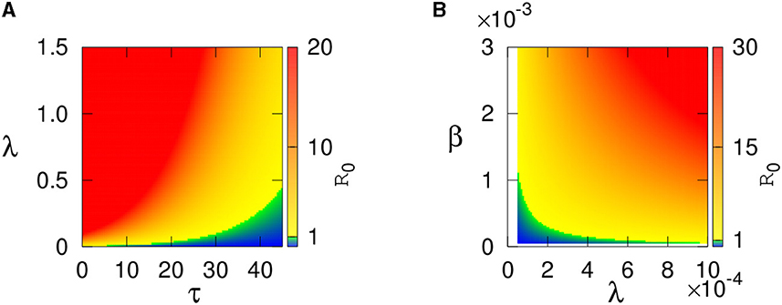
Figure 1. Region of stability of disease-free equilibrium E₂ is shown using the basic reproduction number R₀ depending on (A) τ and λ and (B) β and λ. Color code denotes the values of R₀. The values of the parameters are given in the Table 1.

TABLE 1

Table 1. Parameter values used in numerical simulations [18, 19, 27].

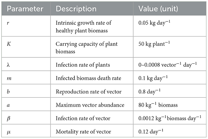
Figure 2 describes how the steady state values of the infected plant and vectors change with R₀. This figure shows that the endemic steady state is stable for lower values of R₀ and then loses its stability via Hopf bifurcation as R₀ exceeds the critical value (following Theorems 5 and 6).

FIGURE 2

Figure 2. (A) Equilibrium values of the infected plant I^* and (B) infected vector V^* population for τ = 0 are plotted. The values of the parameters are taken from Table 1, except λ.

Figures 3, 4 illustrate the model's behavior with τ = 0 and other parameters chosen so that the endemic equilibrium E^* is biologically feasible. When λ < λ^*, the endemic steady state E^* is stable verifying the Theorem 5, as shown in Figure 3, and for λ > λ^*, the Hopf bifurcation has taken place as described in Theorem 6, and, as a result, the system exhibits sustained periodic oscillations shown in Figure 4. Further details of this transition to instability are given in Figure 5, which presents a bifurcation diagram for the endemic steady state E^* depending on the transmission rate λ. A higher transmission rate of the disease can cause instability in the system, and a higher amplitude of oscillations in population densities is seen.

FIGURE 3

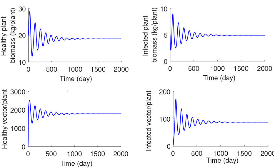
Figure 3. Numerical solution of the system (1) with τ = 0, λ = 0.0003, and other parameter values taken from Table 1.

FIGURE 4

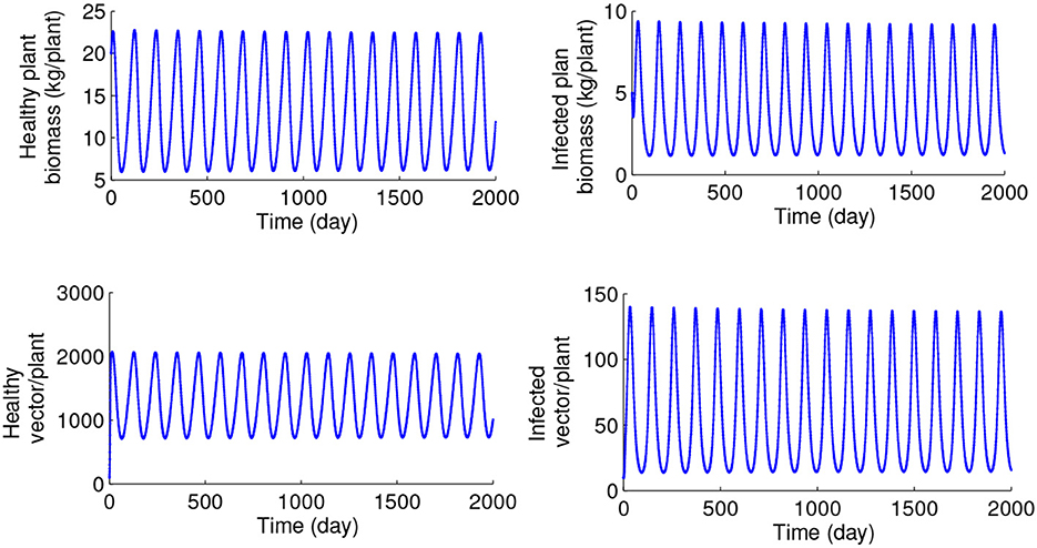
Figure 4. Numerical solution of the system (1) with τ = 0, λ = 0.0006, and other parameter values taken from Table 1.

FIGURE 5

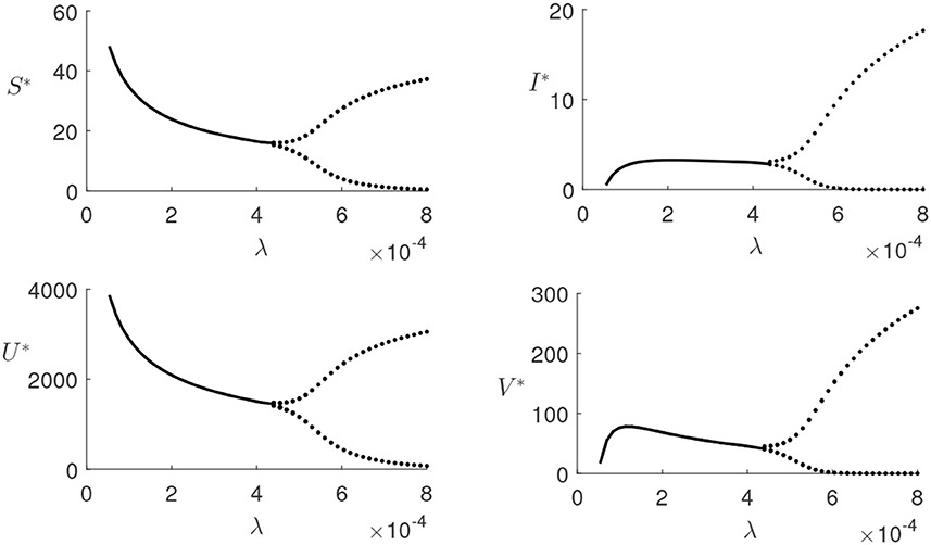
Figure 5. Bifurcation diagram of the endemic steady state E^* without time delay, i.e., for τ = 0, depending on the transmission rate λ, with other parameters taken from Table 1. Dots represent maxima/minima of the respective variables.

Increasing the values of the time delay parameter τ, the stability steady-state E^* is recovered. For a fixed value of plant infection rate λ = 0.0008 (the value at which the endemic steady state E^* is unstable for τ = 0), we have traversed the range of τ and found that for τ≈9.45, this equilibrium regains its stability, and the periodic oscillations disappear (illustrated in Figure 6). The numerical solution of the model for the values of τ exceeding this critical threshold is shown in Figure 7, and it demonstrates that the system converges to the stable steady-state E^*.

FIGURE 6

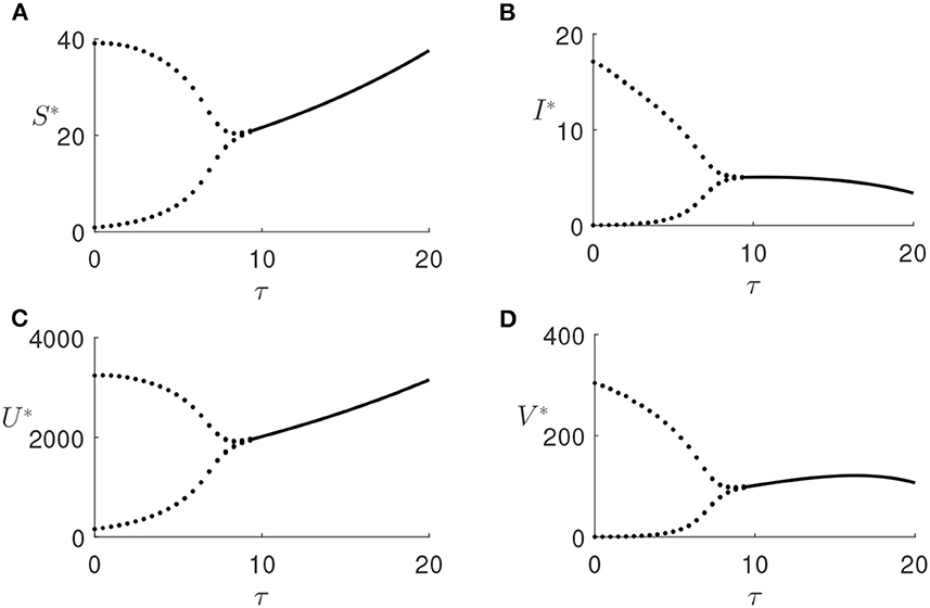
Figure 6. (A–D) Bifurcation diagram of the endemic steady state E^* with λ = 0.0008 and τ as a bifurcation parameter, other parameters are given in Table 1. Dots represent maxima/minima of the respective variables.

FIGURE 7

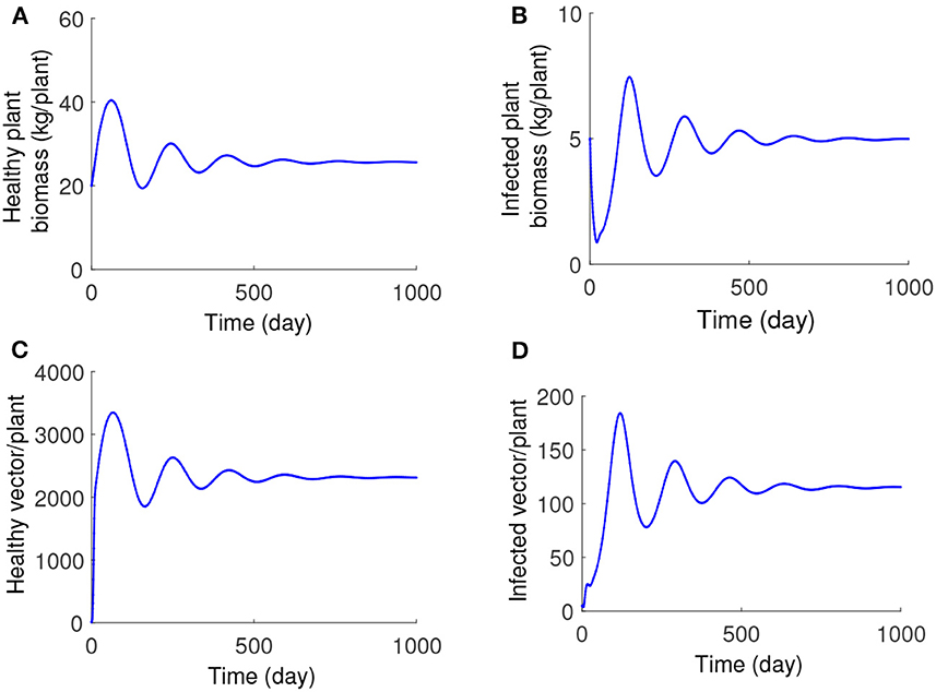
Figure 7. (A–D) Numerical solution of the system (1) with λ = 0.0008, τ = 15, and other parameters as given in Table 1.

Figure 8 illustrates the stability of the endemic steady state E^* depending on different parameters, indicating that E^* is unstable for small τ (which corresponds to high R₀) and stable for larger τ. We also observe that the product of transmission rate λ from vectors to plants and β from plants to vectors has to exceed some threshold value for the endemic steady state to be feasible. For smaller values of this product, the endemic state is stable but also loses its stability via a Hop bifurcation, giving rise to stable periodic oscillations.

FIGURE 8

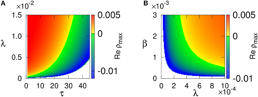
Figure 8. Stability of the endemic steady state E^* with parameters values from Table 1 is shown in (A) τ−λ, and (B) λ−β parameter planes. Color code denotes max[Re(ρ)]. the steady state E^* is not feasible in the white region.

In Figure 9, we plotted the Jacobian matrix's eigenvalues at the endemic equilibria, with τ = 9.45 and λ = 0.0008. A pair of imaginary eigenvalues is observed, indicating a Hopf bifurcation's existence.

FIGURE 9

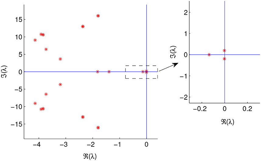
Figure 9. Eigenvalues of the Jacobian matrix evaluated at the endemic equilibrium, E^*, for τ = 9.45, λ = 0.0008, and other parameters values are given in Table 1.

6. Discussion and conclusion

In this study, we have analyzed a time-delayed model for the dynamics of transmission of mosaic disease in J. curcas. Analytical and numerical analyses have provided conditions for the feasibility and stability of various steady states of the model depending on parameters and the time delay. Increasing the rate of disease transmission from vectors to plants destabilizes the disease-free equilibrium through a transcritical bifurcation and the emergence of a stable endemic equilibrium. Interestingly, a further increase of this transmission rate can destabilize the endemic steady state and the emergence of stable periodic oscillations, whose amplitude is growing with the transmission rate.

The time delay can play a dual role: as is often found in time-delayed models, it can by itself lead to a destabilization of the endemic state, but interestingly, it can also provide a mechanism for suppression of oscillations and recovery of stability for the endemic steady state that was otherwise unstable in the absence of the time delays. The numerical solution of the transcendental characteristic equation has provided further insights into how the stability of the endemic steady state depends on parameters, and it has shown that the time delay plays a stabilizing role. It is also seen that increasing either of the transmission rates, i.e., from vectors to plants or from plants to vectors, can result in the loss of stability by the endemic steady state.

Modeling the maturation period as a time delay provides inroads into understanding the stability of disease-free and endemic equilibria by delivering conditions for stability and onset or suppression of oscillations. The time-delayed model effectively captures various aspects of disease dynamics, which can be utilized when collecting and analyzing data from farms, especially when measuring some of the parameters can be difficult.

This model's results provide several important insights for the control and mitigation of the effects of mosaic disease. The basic reproduction number can be computed using values for fundamental parameters describing the specific farming situation. Vector maturation plays an essential role in determining the dynamics of mosaic disease in J. curcas plants. Managers should be aware of the effects of vector maturation time on disease severity and onset of oscillations in the population of infected plants and whitefly vectors. Model predictions concerning particular dynamical regimes depending on parameters provide managers with practical tools for disease monitoring and for developing optimal techniques for successful interventions, including timing and extent of administering protective sprays, insecticides, and fertilizers to reduce crop losses.

Data availability statement

The original contributions presented in the study are included in the article/supplementary material, further inquiries can be directed to the corresponding author.

Author contributions

The author confirms being the sole contributor of this work and has approved it for publication.

Acknowledgments

The author is grateful to Dr. Konstantin Blyuss, University of Sussex, UK for useful discussion during this research.

Conflict of interest

The author declares that the research was conducted in the absence of any commercial or financial relationships that could be construed as a potential conflict of interest.

The reviewer PT declared a past co-authorship with the author to the handling editor.

Publisher's note

All claims expressed in this article are solely those of the authors and do not necessarily represent those of their affiliated organizations, or those of the publisher, the editors and the reviewers. Any product that may be evaluated in this article, or claim that may be made by its manufacturer, is not guaranteed or endorsed by the publisher.

References

1. Soumia PS, Guru Pirasanna Pandi G, Krishna R, Ansari WA, Jaiswal DK, Verma JP, et al. Whitefly-transmitted plant viruses and their management. In: Singh KP, Jahagirdar S, Sarma BK, editors. Emerging Trends in Plant Pathology. Singapore: Springer (2021). p. 175–95.

Google Scholar

2. Adhurya S, Basir FA, Ray S. Stage-structure model for the dynamics of whitefly transmitted plant viral disease: an optimal control approach. Comput Appl Math. (2022) 41:154. doi: 10.1007/s40314-022-01864-9

CrossRef Full Text | Google Scholar

3. Navas-Castillo J, Fiallo-Olivé E, Sánchez-Campos S. Emerging virus diseases transmitted by whiteflies. Annu Rev Phytopathol. (2011) 49:219–48. doi: 10.1146/annurev-phyto-072910-095235

PubMed Abstract | CrossRef Full Text | Google Scholar

4. Saturnino HM, Pacheco DD, Kakida J, Tominaga N, Gonçalves NP. Cultivation of Jatropha curcas L. Inform Agropec. (2005) 26:44–78. Available online at: https://eurekamag.com/research/004/412/004412206.php

Google Scholar

5. Openshaw K. A review of Jatropha curcas: an oil plant of unfulfilled promise. Biomass Bioenergy. (2000) 19:1–5. doi: 10.1016/S0961-9534(00)00019-2

CrossRef Full Text | Google Scholar

6. Mohammad A, Bello I, Maruthi MN, Seal SE, Garga MA. Detection of Jatropha Mosaic Indian Virus (JMIV) on Jatropha Plant (Jatropha curcas). J Adv Res BioChem Pharmacol. (2019) 2:1–4.

PubMed Abstract | Google Scholar

7. Amoatey HM, Appiah AS, Danso KE, Amiteye S, Appiah R, Klu GY, et al. Controlled transmission of African cassava mosaic virus (ACMV) by Bemisia tabaci from cassava (Manihot esculenta Crantz) to seedlings of physic nut (Jatropha curcas L.). Afr J Biotechnol. (2013) 12, 4465–4472. doi: 10.5897/AJB2013.12276

CrossRef Full Text | Google Scholar

8. Leclerc M, Doré T, Gilligan CA, Lucas P, Filipe JAN. Estimating the delay between host infection and disease (incubation period) and assessing its significance to the epidemiology of plant diseases. PLoS ONE (2014) 1:e86568. doi: 10.1371/journal.pone.0086568

PubMed Abstract | CrossRef Full Text | Google Scholar

9. Al Basir F, Kyrychko YN, Blyuss KB, Ray S. Effects of vector maturation time on the dynamics of cassava mosaic disease. Bull Math Biol. (2021) 83:87. doi: 10.1007/s11538-021-00921-4

PubMed Abstract | CrossRef Full Text | Google Scholar

10. Buonomo B, Cerasuolo M. The effect of time delay in plant-pathogen interactions with host demography. Math Biosci Eng. (2015) 12:473–90. doi: 10.3934/mbe.2015.12.473

PubMed Abstract | CrossRef Full Text | Google Scholar

11. Erneux T. Applied Delay Differential Equations. New York, NY: Springer (2009).

Google Scholar

12. Kuang Y. Delay Differential Equations with Applications in Population Dynamics. New York, NY: Academic Press (1993).

Google Scholar

13. Van der Plank JE. Plant Diseases: Epidemics and Control. New York, NY: Academic Press (1963).

Google Scholar

14. Jeger MJ, Holt J, van den Bosch F, Madden LV. Epidemiology of insect-transmitted plant viruses: modelling disease dynamics and control interventions. Physiol Entomol. (2004) 29:291–304. doi: 10.1111/j.0307-6962.2004.00394.x

CrossRef Full Text | Google Scholar

15. Jackson M, Chen-Charpentier BM. A model of biological control of plant virus propagation with delays. J Comput Appl Math. (2018) 330:855–65. doi: 10.1016/j.cam.2017.01.005

CrossRef Full Text | Google Scholar

16. Jackson M, Chen-Charpentier BM. Modeling plant virus propagation with delays. J Comput Appl Math. (2017) 309:611–21. doi: 10.1016/j.cam.2016.04.024

PubMed Abstract | CrossRef Full Text | Google Scholar

17. Neofytou G, Kyrychko YN, Blyuss KB. Time-delayed model of immune response in plants. J Theor Biol. (2016) 389:28–39. doi: 10.1016/j.jtbi.2015.10.020

PubMed Abstract | CrossRef Full Text | Google Scholar

18. Al Basir F, Venturino E, Roy PK. Effects of awareness program for controlling on mosaic disease in Jatropha curcas plantations. Math Methods Appl Sci. (2017) 40:2441–53. doi: 10.1002/mma.4149

CrossRef Full Text | Google Scholar

19. Venturino E, Roy PK, Al Basir F, Datta A. A model for the control of the mosaic virus disease in Jatropha curcas plantations. Energy Ecol Environ. (2016) 1:360–9. doi: 10.1007/s40974-016-0033-8

CrossRef Full Text | Google Scholar

20. Al Basir F, Roy PK. Dynamics of mosaic disease with roguing and delay in Jatropha curcas plantations. J Appl Math Comput. (2018) 58:1–31. doi: 10.1007/s12190-017-1131-2

CrossRef Full Text | Google Scholar

21. Duffus JE. Whitefly transmission of plant viruses. In: Harris KF, editor. Current Topics in Vector Research. New York, NY: Springer (1987). p. 73–91.

Google Scholar

22. Costa AS. Whitefly-transmitted plant diseases. Annu Rev Phytopathol. (1976) 14:429–49.

Google Scholar

23. Hale J. Theory of Functional Differential Equations. New York, NY: Springer-Verlag (1977).

Google Scholar

24. Heffernan JM, Smith RJ, Wahl LM. Perspectives on the basic reproductive ratio. J. R. Soc. (2005) 2, 281–293. doi: 10.1098/rsif.2005.0042

PubMed Abstract | CrossRef Full Text | Google Scholar

25. Murray JD. Mathematical Biology. I. An Introduction. New York, NY: Springer (2002).

Google Scholar

26. Breda D, Maset S, Vermiglio R. Pseudospectral approximation of eigenvalues of derivative operators with non-local boundary conditions. Appl Numer Math. (2006) 56:318–31. doi: 10.1016/j.apnum.2005.04.011

CrossRef Full Text | Google Scholar

27. Holt J, Jeger MJ, Thresh JM, Otim-Nape GW. An epidemiological model incorporating vector population dynamics applied to African cassava mosaic virus disease. J Appl Ecol. (1997) 34:793–806.

Google Scholar