Fusing time-varying mosquito data and continuous mosquito population dynamics models

Climate change is arguably one of the most pressing issues affecting the world today and requires the fusion of disparate data streams to accurately model its impacts. Mosquito populations respond to temperature and precipitation in a nonlinear way, making predicting climate impacts on mosquito-borne diseases an ongoing challenge. Data-driven approaches for accurately modeling mosquito populations are needed for predicting mosquito-borne disease risk under climate change scenarios. Many current models for disease transmission are continuous and autonomous, while mosquito data is discrete and varies both within and between seasons. This study uses an optimization framework to fit a non-autonomous logistic model with periodic net growth rate and carrying capacity parameters for 15 years of daily mosquito time-series data from the Greater Toronto Area of Canada. The resulting parameters accurately capture the inter-annual and intra-seasonal variability of mosquito populations within a single geographic region, and a variance-based sensitivity analysis highlights the influence each parameter has on the peak magnitude and timing of the mosquito season. This method can easily extend to other geographic regions and be integrated into a larger disease transmission model. This method addresses the ongoing challenges of data and model fusion by serving as a link between discrete time-series data and continuous differential equations for mosquito-borne epidemiology models.

1. Introduction

Climate change is arguably one of the most pressing issues affecting our world today, and one of the threats exacerbated by the changing climate is mosquito-borne disease transmission [1, 2]. Mosquito-borne diseases such as malaria, dengue, and West Nile virus are transmitted through the bites of infectious female mosquitoes and are responsible for 350–650 million human cases and over 630,000 deaths worldwide each year [3, 4]. Mosquito populations are directly impacted by climatic variables, such as air temperature and precipitation, in a non-linear way [5–7]. The air temperature needs to be warm enough for mosquitoes to survive and develop, but if too hot can cause excess mortality [8, 9]. Precipitation is necessary to create egg laying sites for juvenile mosquitoes, but too much rainfall can risk flushing eggs and larvae from their habitats [10, 11]. A comprehensive approach that incorporates data streams for climate, land cover, and mosquito and human populations is vital to predict the next mosquito-borne disease outbreak and assess mitigation strategies [2]. Many mosquito-borne disease transmission models that incorporate known biological mechanisms and allow for “what-if” scenarios are continuous and either autonomous [12–15] or vary with a function such as a sine wave [16]. The former is good for single-season outbreaks and building intuition, while the latter may capture seasonal patterns with tractable analysis [17]. However, neither approach captures inter-annual and intra-annual variation in season length and intensity when they are not directly connected to observed data [2, 18]. To better understand how mosquito-borne disease transmission will be altered under climate change, we aim to incorporate variable seasonal dynamics of mosquito populations into a classical mathematical model for mosquito population dynamics.

As we gain access to increasingly diverse and big data, we have the opportunity to merge data-driven and model-driven approaches to enhance our understanding of physical and biological phenomena [19]. An ongoing challenge of integrating both approaches is data fusion—the process of transforming collected data into a usable format [2] to reconcile disparate data streams of varying spatial and temporal resolution. Further, data fusion needs for connecting discrete, noisy data to mechanistic mathematical models differ from the data fusion needs for purely statistical models [19]. In the context of understanding mosquito population dynamics as informed by climate and environment, mosquito trap data is currently the gold standard for capturing within and between season variation mosquito density in a particular location [20]. Additionally, some highly detailed mosquito life cycle models [21, 22] can produce predictions of mosquito populations variation through time. Data from traps or high-resolution model output are discrete and often noisy, varying widely between and within seasons [23]. Recovering time-varying parameters from time-series data is an ongoing endeavor related to the area of determining dynamics [24, 25]. Existing methods tend to be computationally intensive or produce outputs that are difficult to interpret [18, 26]. A current challenge is to incorporate this important data-driven variability into disease transmission models while preserving the fast computation time, interpretability, and general utility of a continuous differential equation approach [2, 27].

To address this question, we annually fit a non-autonomous logistic model with periodic net growth rate and carrying capacity parameters to 15 years of mosquito time-series data from the Greater Toronto Area of Canada. We considered ten variations of the non-autonomous logistic growth model, allowing for different combinations of fixed and varying parameters to ensure a balance between parsimony and enough flexibility to capture observed patterns throughout the considered time period. We used a model selection procedure, Akaike Information Criterion (AIC), to show that a four-parameter non-autonomous logistic model best captures the dynamic behavior for two types of adult female mosquito time-series data, (a) the Total Population including all adult female stages, and (b) the Active Population—blood-seeking females assumed to be directly proportional to number of captures per trap per day. We also quantified model error and determined not only optimal parameters for each year, but also the best start and end days of the mosquito season as these vary from year to year. We further explore the sensitivity of parameters on the peak magnitude and timing of the mosquito season for each population type. This method addresses the ongoing challenges of data and model fusion by serving as a link between a discrete, noisy population time series and continuous differential equations for mosquito-borne epidemiology models.

2. Methods

2.1. Non-autonomous logistic model with periodic parameters

The logistic growth model is often used to model density-dependent population dynamics, including mosquitoes [12, 28, 29]. Under logistic growth, the population's rate of change decreases linearly as its size approaches the carrying capacity. The carrying capacity is the theoretical maximum that can be sustained by the environment. These logistic growth models can be used to assess population control strategies, or incorporated into a larger, mechanistic vector-borne disease modeling framework to study transmission dynamics [12, 13, 30]. The classical logistic model and many applications assume that the biological parameters– the intrinsic growth rate and carrying capacity– are constant with respect to time [13]. This simplifying assumption not only allows for increased mathematical tractability and analysis, but also serves as an approximation when detailed, reliable population data is unavailable. However, the assumption of constant parameters may fail to capture realistic behavior observed in nature, particularly in the case for mosquitoes whose populations are inherently time-dependent [8, 10, 11]. Specifically, the mosquito population growth rate is known to be influenced by temperature and carrying capacity depends on the availability of egg laying sites and competition between larvae [12].

The classic non-autonomous logistic model consists of a single ordinary differential equation to represent the population of adult female mosquitoes, P(t):

$\begin{array}{ll}\frac{dP(t)}{dt}=r(t)P(t)(1-\frac{P(t)}{K(t)}),& (1.1)\end{array}$

where r(t) is the time-varying intrinsic net growth rate and K(t) is the time-varying carrying capacity. For this application, the net growth rate is defined as the difference between the rates of adult emergence and adult mortality. Therefore, it is possible for the net growth rate to be negative. Such examples of a negative growth rate can occur during extreme weather events that kill a high proportion of juvenile or adult mosquitoes, or could just be typical environmental patterns that cause some species of mosquitoes to diapause during the winter season [31]. The model assumes both growth rate and carrying capacity are time-varying since both processes are influenced by time-dependent exogenous factors, such as temperature, water availability, and daylight hours [8, 10, 11]. We use periodic functions to represent the yearly seasonal fluctuations of r(t) and K(t):

$\begin{array}{ll}r(t)=r_b-r_s\text{cos}(\frac{2\pi t}{365}),& (1.2)\end{array}$

$\begin{array}{ll}K(t)=K_b-K_s\text{cos}(\frac{2\pi t}{365}).& (1.3)\end{array}$

Components with the b subscripts denote the baseline (mean) values, and the components with s subscripts represent the amplitude scaling factor of the cosine wave.

2.2. Data and mosquito process-based model

Greater Toronto Area (GTA) mosquito data for years 2005–2016 was obtained from Public Health Ontario's mosquito database. Adult mosquitoes are trapped weekly during the mosquito season, which occurs from roughly May–October for Toronto. This time frame recorded over 115,000 mosquito observations from 2,722 trap sites. Since nearly 85% of the traps used were Light Traps targeting female mosquitoes actively seeking a blood meal, we assume in the models that all trapped mosquitoes are female and blood-seeking. The majority of identified mosquitoes were Culex pipiens and Culex restuans species, which are known to transmit West Nile virus (WNV) [21]. The data from the WNV mosquito database is available upon request and approval from Public Health Ontario [32].

Our non-autonomous logistic model is capable of fitting any discrete time series for mosquitoes. However, in this study, to overcome the challenges of sparse trap data and outliers, our non-autonomous logistic model was fitted to the daily output from a Process Based Model (PBM) developed by Shutt et al. [21]. Shutt et al.'s PBM mechanistically models the life stages of mosquitoes and provides an improved estimation of the daily true mosquito population compared to fitting parameters to the temporally-coarse data alone. The PBM was fitted to the GTA's Culex trap data for years 2005–2016, and we used it to estimate the mosquito populations for years 2017–2019 based on temperature and stream gauge records. The PBM provides two time-series outputs—the Total Population, representing the adult female mosquito total count in the GTA each day (including mosquitoes meal-seeking, resting, egg-laying, and in diapause), and the blood-seeking female mosquito Active Population, assumed to be directly proportional to the average number of captures per trap per day. Although our non-autonomous logistic linkage model is being fitted to the output from a high-fidelity mosquito life cycle model, it also has the capability to fit any discrete time series for mosquitoes, such as trap data.

2.3. Model selection procedure

Model selection involves finding a balance between having a model detailed enough to capture important behavior of interest, but not so detailed that it overfits the given dataset. In order to find a non-autonomous logistic model best fits the data across all years, we conducted a model selection procedure using the Akaike Information Criterion (AIC) [33]. The AIC is based on information theory and discourages overfitting by penalizing models with more parameters. Models with a smaller AIC can reflect better goodness-of-fit over models with larger AIC.

Ten candidate models of hierarchical nature were included in the model selection procedure (Table 1). Each candidate model fits a subset of the parameters of model (1) while keeping the remainder of the parameters fixed. The first four models (A–D) assume a constant carrying capacity (i.e., K_s = 0), and the last six models (E–K) assume a time-varying carrying capacity.

TABLE 1

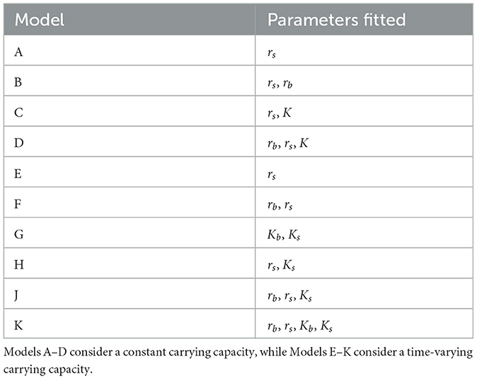
Table 1. Candidate models for the model selection procedure.

Parameter fitting was carried out in Python using the least_squares function from the SciPy Optimize library [34]. This function minimizes the mean squared error between the PBM output and our model simulation. We use a Trust Region Reflective algorithm for minimization, which allows us to incorporate bounds on the parameter search space as described in Supplementary Table 1. Further details about the selected search space constraints are included in Section 2.4. Simulation of the model (1) uses a fourth-order Runge-Kutta method.

The parameters for each candidate model were fitted for three tests for each mosquito population (Total and Active). We refer to these tests as “Fitting Seasons”, that roughly represent the duration and timing of mosquito prevalence in the GTA. The three Fitting Seasons for the Total Population occur from (i) May 1–October 1, (ii) May 15–October 15, and (iii) June 1–November 1, each year. Each of the Fitting Seasons last 154 days, or 22 weeks. The Total Population time-series pose a challenge when fitting the non-autonomous logistic model from November to May since this is the period during which most or all adult female mosquitoes are in diapause. However, it is assumed that since the majority of the mosquitoes remain in a diapause state during this time frame they are less relevant to model for disease transmission or vector control modeling purposes. On the other hand, the Active Population can be modeled throughout the full year (365 days) without issue. The three Fitting Seasons for the Total Population begin (i) May 1, (ii) May 15, and (iii) June 1, each year.

For each population, the AIC for candidate model j= A, B,..., K was calculated from the sum of squared errors (SSE) over all M = 15 years of time-series data [33]:

$\begin{array}{ll}{\text{AIC}}_j=n\left[ln(\frac{{\text{SSE}}_j}{n})\right]+2(k+1),& (2)\end{array}$

where,

$\begin{array}{l}{\text{SSE}}_j={\displaystyle \sum _{i=1}^M}{\text{SSE}}_i^j,\end{array}$

is the sum of the SSE for years i = 1, 2, ...M for candidate model j, n is the number of data points (154 fitting days × M years for Total Population, 365 fitting days × M years for Active Population), and k is the number of parameters fitted.

2.4. Parameter optimization

The four-parameter model (Model K) was selected as it produced the lowest AIC for each of the three Fitting Seasons for both Total and Active Populations. We then estimated the seasonal (yearly) net growth rate and carrying capacity parameters for the Total and Active Populations of the GTA from 2005–2019 using Model K from the Model Selection Procedure. Similar to the process that fitted parameters for the Model Selection Procedure, a Trust Region Reflective algorithm from the SciPy Optimize library [34] found the optimal seasonal parameters for the time-varying net growth rate and carrying capacity. Specifically, the components r_b, r_s, K_b, and K_s of (1.2)–(1.3) were found for each of the 15 seasons for each population type. The Trust Region Reflective algorithm allows us to incorporate bound constraints for parameters based on estimated ranges for the net growth rate [12, 13, 35] and reasonable assumptions for the carrying capacity [36]. This algorithm is a least squares method, which minimizes the mean squared error between the PBM time-series and the mosquito population P(t). Other methods to infer parameters from data include gradient descent [37], Bayesian inference [23, 38], and ensamble-adjusted Kalman filter [39]. Each of these methods are suitable for fitting a small number of model parameters, but we used the Trust Region algorithm to incorporate biologically suitable parameter bounds [34]. This framework relates to the concept of determining dynamics by providing a useful way to connect discrete time-series data to numerous time-varying parameters from a continuous modeling framework [18, 24–26].

2.4.1. Total mosquito population

As mentioned earlier, the Total Mosquito Population includes all adult female mosquitoes in the GTA—i.e., the Total Population captures the amount of adult female mosquitoes through all stages of the gonotrophic cycle—bloodmeal seeking, digestion and egg maturation, and oviposition—as well as those in diapause. The start and duration of the optimal mosquito fitting season for the Total Population changes from year-to-year and reflects the interannual variation of mosquito populations. The majority of mosquitoes remain dormant in diapause during the cold winter and emerge once temperatures become suitable for growth and survival [21]. Mosquitoes in diapause remain non-biting, and thus do not pose a risk for contributing to infection propagation [31]. We explored May 1–June 1 as “candidate start days” to begin fitting the Total Population each year. The range of “candidate start days” refers to the time when mosquitoes begin to emerge from their overwintering state in the GTA. Similarly, “candidate end days” refer to the range of dates when most mosquitoes are likely to be in diapause. We selected October 1–November 1 as the date range for the “candidate end days.” The range of candidate start and end days provides an exhaustive grid-search across the likely emergence and disappearance of mosquitoes for each season.

For each year, the initial condition, P(0), was selected as the value of the mosquito PBM time-series on the candidate start day. The initialized value of K_b was selected as the maximum of the mosquito PBM time-series between the candidate start day and candidate end day. The bound constraints for the parameters were selected as −0.2 ≤ r_b ≤ 0.2, −0.35 ≤ r_s ≤ 0, 1 ≤ K_b ≤ 100, 000, and 0 ≤ K_s < 100, 000. Bound constraints for the growth rate parameters were estimated from previous modeling studies [12, 13, 35] and were included to mitigate the problem of obtaining biologically irrelevant values. Although less is known about the bound constraints for the carrying capacity parameters, we assumed the carrying capacity to be no more than one order of magnitude larger than the largest observation of the mosquito PBM time-series. Parameters r_b and r_s were initialized as r_b = 0 and r_s = −0.07 to provide a biologically relevant starting place for optimization. Parameter K_s was arbitrarily initialized as 0.1% of the maximum baseline carrying capacity (i.e., K_s = 100) to reflect a small variation in carrying capacity. The selected parameter initialization and constraints directs the optimization algorithm to an appropriate solution—one that is both biologically valid and numerically stable.

Each of the 14,415 fits (31 candidate start days × 31 candidate end days × 15 years) returns the fitted parameters along with the root mean squared error (RMSE). The combination of the candidate start day and candidate end day with the lowest RMSE for each year is selected as that year's mosquito fitting season. The resulting r_b, r_s, K_b, and K_s values obtained from the mosquito fitting season determine the time-varying net growth rate and carrying capacity parameters for that year.

2.4.2. Active mosquito population

The Active Mosquito Population represents the number of adult female mosquitoes in the GTA currently seeking a blood meal in their gonotrophic cycle, so are assumed to be most likely to be trapped. In other words, this is the population of mosquitoes that are actively biting humans and other animals, and provides a reasonable estimate for understanding the magnitude of mosquito-borne disease risk on a given day. The fitting season of the Active Population lasts 365 days since they go down to zero during the winter, which the model can easily capture (as opposed to the Total Population time series that includes diapausing mosquito dynamics during winter which we avoided fitting to). The range of “candidate start days” were chosen from May 1–June 1 each year and fitted until the same calendar day the following year. That is, new values for r_b, r_s, K_b, and K_s are fitted every 365 days.

To ensure the mosquito population remains non-negative, the initial condition, P(0), was selected as maximum between 0.01 and the mosquito PBM value on the candidate start day. The initialized value of K_b was the maximum value of the mosquito PBM time-series during the fitting season. The carrying capacity for the Active Population is much lower than that of the Total Population because it is scaled to the number of adult female mosquitoes captured per trap per day, rather than the entire population. Therefore, we reasonably assumed the bound constraints for K_b and K_s to be 1 ≤ K_b ≤ 1, 000 and 0 ≤ K_s < 1, 000, respectively. Initialization and bound constraints for r_b and r_s are as before, and K_s initialized as 0.1% of the maximum K_b value (i.e., K_s = 1).

The root mean squared error (RMSE) was found for each of the 465 fits (31 candidate start days × 15 years), and candidate start day with the lowest RMSE value for each year was selected as that season's start day. For each year, simulations last from the current season's start day until the following season's start day. That is, the 365 day period used to fit the model is extended/truncated to align with the next season's start day. The last season of the time-series is simulated for the full 365 day period from the season's start day. This produces a piecewise-continuous function to approximate the Active Population across the 15 years of time-series data.

2.5. Sensitivity analysis

A sensitivity analysis was conducted to better understand the influence of non-autonomous logistic model parameters on two quantities of interest. The quantities of interest we explored were the peak magnitude and peak timing. The peak magnitude is defined as the greatest daily mosquito population simulated within a season [maxP(t)], and the peak timing is the time t at which the peak occurs. Sobol sensitivity indices [40] of each parameter were computed for the peak magnitude and timing of the Total and Active Populations. Sobol sensitivity analysis is a variance-based sensitivity measure which computes the percentage of variance that can be attributed to each input parameter and their interactions [40, 41].

For each population type (Total and Active), we generated 1,024 (or 2¹⁰) samples of parameter combinations for the Sobol sensitivty analysis using the sobol.sample function of the SALib sample package [42, 43]. To avoid selecting samples that would be biologically invalid, we first re-scaled the carrying capacity equation (1.3) to ensure that the model would always produce a non-negative carrying capacity:

$\begin{array}{ll}K(t)=K_b(1-K_{a}cos(\frac{2\pi t}{365})),& (3)\end{array}$

where 0 < K_a < 1. Sensitivity indices were computed for five model parameters: the baseline and scaling net growth rate parameters (r_b and r_s), the baseline and re-scaled carrying capacity parameters (K_b and K_a), and the initial condition P(0). Parameter ranges for r_b, r_s, K_b, and P(0) were selected from the ranges obtained from the parameter fitting results of each population type (see Sections 3.2, 3.3, along with Supplementary Tables 2, 3). We decided to use these ranges for the parameter sampling bounds instead of the original ranges selected for the parameter fitting (see Sections 2.4.1, 2.4.2) because certain combinations of parameters could produce numerically unstable output. In particular, numerical simulations tended to be unstable when large carrying capacity fluctuations were selected with large net growth rate values. Because of this, we limited the range of K_a values to be between 0 and 0.9.

Simulations of the non-autonomous logistic model were run for 184 days for the Total Population and 300 days for the Active Population for each parameter sample. The time frame for the Total Population aligns with the time frame used for fitting parameters (May 1–Nov 1), and the time frame for the Active Population was selected to ensure that only one peak would be generated during the period of simulation. The peak magnitude and timing was computed from each simulation for both populations, and the first and total order Sobol sensitivity indices were found using the sobol.analyze function of the SALib sample package [42, 43]. First order indices measure the contribution to output variance by a single model input alone, while the total order indices measure the contribution to the output variance caused by the model input and all higher order interactions with other model inputs [40, 43].

3. Results

3.1. Model selection

Akaike Information Criterion (AIC) values from the three tests for the Total and Active Populations in the GTA are shown in Tables 2, 3, respectively. For both populations, the four-parameter model, Model K, has the lowest AIC value out of the ten candidate models for each test. The three-parameter model with constant carrying capacity, Model D, also performs relatively well for both populations. Model G, the two-parameter model with time-varying carrying capacity, performs fairly well for the Total Population when the fitting season occurs from May 1–October 1, but has poor performance when fitting from June 1–November 1. Since the fitting season will vary slightly from year-to-year, Model K was selected to ensure a better fitting quality throughout the range of potential fitting seasons.

TABLE 2

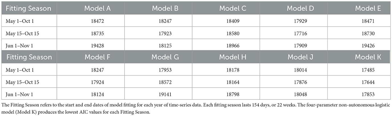
Table 2. Akaike Information Criterion (AIC) values from the 10 candidate models of Greater Toronto Area's Total Mosquito Population.

TABLE 3

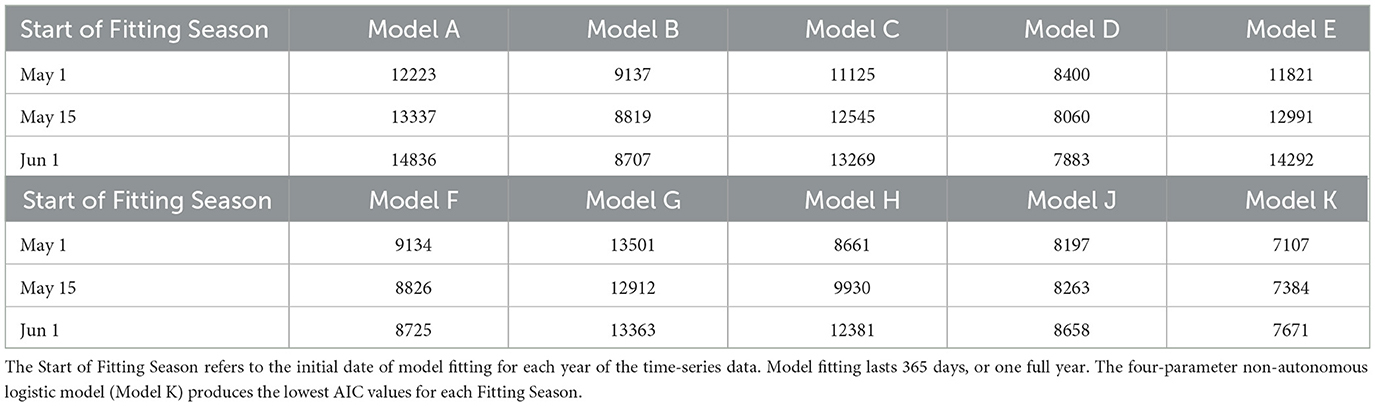
Table 3. Akaike Information Criterion (AIC) values from the 10 candidate models of Greater Toronto Area's Active Mosquito Population.

3.2. Parameter fitting results for Total Population

Parameter fitting results for the GTA's Total Population is show in Figure 1. Figure 1A shows the seasonal fittings of the model (1) along with the mosquito PBM output. Figure 1B shows the relative root mean squared error (RRMSE) values for each year's optimal fit. Although the mean squared error metric was used as the cost function for parameter optimization, RRMSE values are presented in Figure 1B to provide comparison of the fitting performance across years. Different parameters were fitted separately for each year due to the deterministic nature of the model and yearly variation in the data. Nipa et al. used a stochastic differential equation model with seasonality incorporated for the mosquito population in a dengue transmission model [16]. However, selecting similar seasonal constants as our method can be achieved through averaging numerous realizations of this stochastic model, but would be more computationally intensive.

FIGURE 1

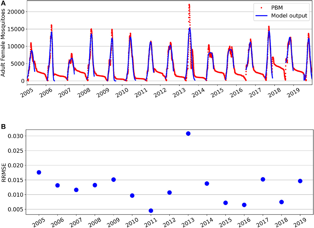
Figure 1. Fitting results for the Greater Toronto Area's Total Mosquito Population for years 2005–2019. (A) Simulations of model fittings (blue curves) and Mosquito Process-Based Model output (red dots). (B) Relative root mean squared error values.

For the Total Population, it can be observed that the PBM time-series exhibits a “tail” toward the end of each mosquito season. This occurs during the period from November through April, where the majority of Culex mosquitoes in the GTA remain dormant in a diapause state. During diapause, female mosquitoes are neither biting nor seeking a bloodmeal, and are therefore not at risk for spreading infection [31]. The non-autonomous logistic model fits the PBM time-series data during the period when mosquitoes have emerged from diapause, which occurs roughly between May and October for the GTA.

Supplementary Figure 1 provides a closer look at each year's best fit. Overall, the time-varying parameters of the non-autonomous logistic model are able to capture the intraseasonal and interannual variability of the Total Mosquito Population. However, the model fitting struggles to capture the peak magnitude of for some seasons—particularly for years 2007 and 2014 which both had multiple peaks during the mosquito season. Year 2013 had the lowest fitting performance and is also the year with the greatest peak value and a distinctly bi-model mosquito season. The substantial increase of peak magnitude for 2013 is likely attributed to unusually high flooding in the GTA for that year [44]. The model (1) was not fitted to the Total Population data from late fall through early spring, as it was assumed that the majority of adult female mosquitoes during this period were in diapause. The mosquito fitting season and fitted parameter values for each year are found in Supplementary Table 2. We note that the minimum carrying capacity value throughout the season is always non-negative. Interestingly, nearly half of the years (7 of 15, K_s≈0) show a nearly constant carrying capacity throughout the mosquito fitting season, while other years show larger variability in the carrying capacity where K_s ranges from 31 to 99% of the baseline value. This explains why the three-parameter model with constant carrying capacity was the second best performing model after the four-parameter model with time-varying carrying capacity.

The difference in optimal candidate start and end date combinations between years 2011 and 2014 highlight the intra-seasonal variation in mosquito populations within a geographical location, as is apparent in the heatmaps of Figure 2. The heatmaps present the normalized RMSE to best compare the fitting performance across start and end date combinations within a single year. For 2011, Fitting performance is optimal when the Mosquito Fitting Season begins the first week of May and ends the first week of October. In 2014, a Mosquito Fitting Season from late May to mid October provides the best fit. Heatmaps of normalized RMSE values for GTA's Total Population for years 2005–2019 are shown in Supplementary Figure 2.

FIGURE 2

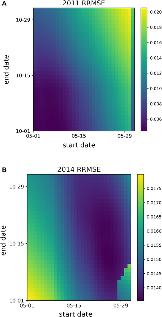
Figure 2. Heatmaps of the normalized root mean squared error (RMSE) values from Total Population fittings with respect to candidate start and end dates for years (A) 2011 and (B) 2014. Dark purple regions denote the candidate start and end date combinations with the lowest normalized RMSE values.

3.3. Parameter fitting results for Active Population

Parameter fitting results for the GTA's Active Population are shown in Figure 3. Figure 3A shows the seasonal fittings of the model (1) along with the mosquito PBM output. Figure 3B shows the RRMSE values for each year's optimal fit. A more detailed look at each year's best fits is provided in Supplementary Figure 3. The model can accurately capture the peak magnitude for most of the mosquito seasons. The model may struggle to capture peaks that have greater magnitudes or additional non-linear qualities due to requiring a steeper derivative of the differential equation and potentially causing stability issues of the numerical solver. Additionally, a clear discontinuity is observed between the end of the 2011 season and the beginning of the 2012 season, showing that the model may not always provide a smooth, continuous simulation from year-to-year. Nonetheless, the model simulation generally avoids the noise in the time-series values that occurs at the beginning of the season as mosquitoes are emerging somewhat sporadically.

FIGURE 3

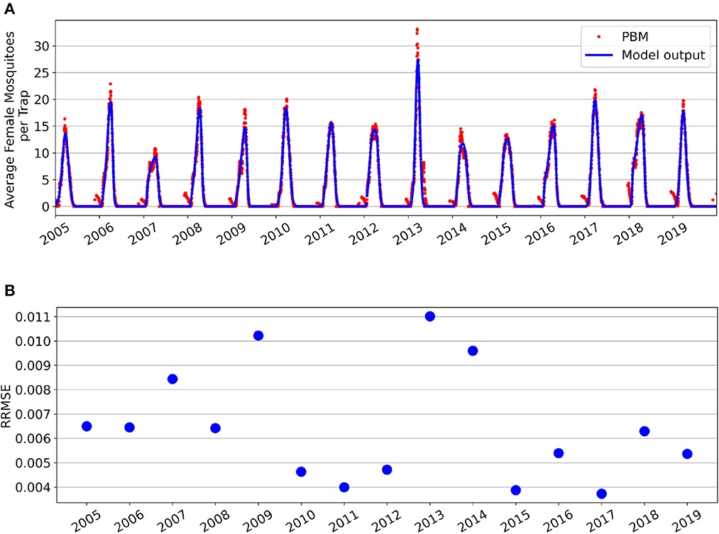
Figure 3. Fitting results for the Greater Toronto Area's Active Mosquito Population for years 2005–2019. (A) Simulations of model fittings (blue curves) and Mosquito Process-Based Model output (red dots). (B) Relative root mean squared error values.

Supplementary Table 2 provides the optimal fitted parameters for each season. Similarly to what we observed for the Total Population, the minimum carrying capacity for each season is non-negative, and 6 of 15 years show a constant carrying capacity. Interestingly, five of the years with constant carrying capacity were the same for both Total and Active Populations.

Intraseasonal variation of the model fitting performance by start date is shown in Figure 4 for the 2013 (Figure 4A) and 2019 (Figure 4B) seasons. Similarly to what was observed for the Total population, the season start date of the Active population varies year-to-year. The start date of the fitting season directly relates to the peak magnitude achieved in the simulation. May 20th as the optimal start date for the 2013 season, and May 1st as the optimal start date for the 2019 season. Intraseasonal variation for the Active Mosquito Population for all years 2005–2019 is included in Supplementary Figures 4, 5.

FIGURE 4

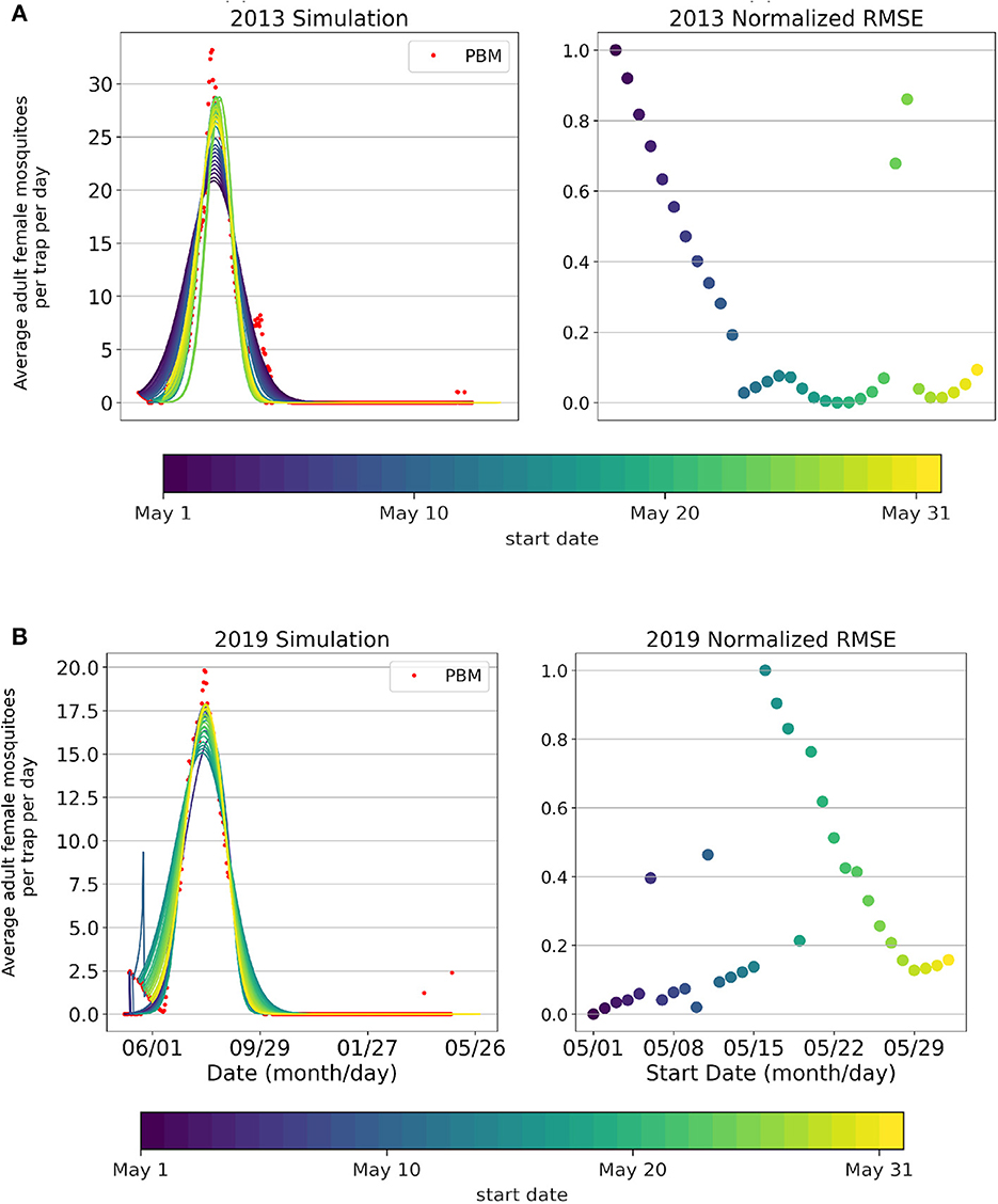
Figure 4. Simulations (curves) of the Active Mosquito Population, Mosquito Process-Based Model output (red dots), and normalized root mean squared error values for each start date's fitting (May 1st-June 1st) for years (A) 2013 and (B) 2019.

3.4. Sensitivity analysis

Sensitivity results of the parameters are displayed in Figure 5 for the peak magnitude (Figure 5A) and peak timing (Figure 5B) of the Total and Active Populations of the GTA. The first order effects measure the single model input's contribution to the output variance, and the interaction order effects measure the higher order interactions between model input combinations [40]. The interaction order effects were found by taking the difference between the total order and first order effects.

FIGURE 5

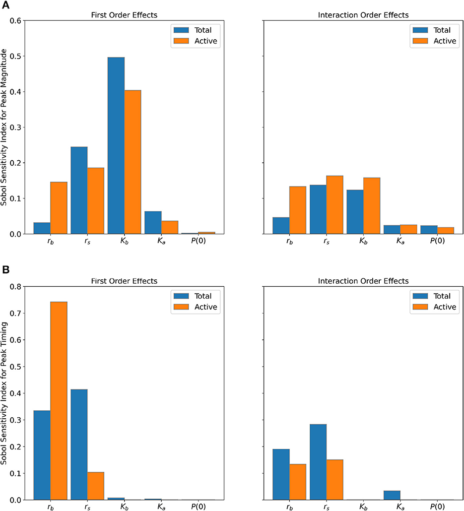
Figure 5. Sensitivity of (A) peak magnitude and (B) peak timing to parameters for the Total (blue bars) and Active (orange bars) Populations. Interaction order sensitivities were found by taking the difference between the total order and first order effects.

The baseline carrying capacity (K_b) is the most sensitive parameter for the peak magnitude for both populations (Figure 5A), followed by the variation in net growth rate (r_s)—between 40 and 50% of the output variance is explained by K_b alone, and 18-25% of the variance is explained by r_s alone. We notice that the baseline net growth rate (r_b) has greater first and interaction order effects for the Active Population compared to the Total Population for peak magnitude. The other parameters display similar interaction order effects between the two populations for the peak magnitude.

For peak timing (Figure 5B), both populations show the greatest sensitivity to the net growth rate parameters (r_b and r_s). However, the Active Population has substantially greater first order effects for r_b and less sensitivity to r_s compared to the Total Population. Nearly 88% of the output variance can be attributed to r_b alone for the Active Population, compared to only 53% for the Total Population. On the other hand, roughly 70% of output variance is attributed to r_s for the Total Population, whereas only 25% for the Active Population.

Discrepancies in sensitivity indices between the two populations are likely the result of the slightly different parameter ranges used in the parameter sampling. These differing parameter ranges were selected based on the differing characteristics of each population time-series. When compared to the Active Population, the fitted baseline carrying capacities and initial conditions for the Total Population were up to two and four orders of magnitude greater, respectively (see Supplementary Tables 2, 3). Further investigation of parameter identifiability and sensitivity may yield additional explanation about these differences [41, 45]. Nonetheless, both population types clearly show that the peak magnitude is most sensitive to K_b and r_s, while the peak timing is most sensitive to r_b and r_s. This suggests that the fluctuations in net growth rate drive both peak magnitude and timing of the mosquito season. Furthermore, the baseline carrying capacity is most influential for the peak size, and the baseline net growth rate is most influential for the timing of the peak.

4. Discussion

As data availability and storage continue to expand, data-driven mechanistic and mathematical models provide useful insights into the dynamics of various biological processes, such as population growth [18, 20]. Mosquito populations have seasonal fluctuations dependent on non-linear, exogenous variables related to climate, land cover, and human behavior [2, 10, 46], and is an ongoing challenge. The ability to accurately quantify mosquito populations is important—not only to understand their distribution across various spatial and temporal scales, but also to inform vector-borne disease control and mitigation efforts, particularly under the continued threat of climate change [6, 23, 38].

In this study, we fitted a non-autonomous logistic model with piecewise periodic net growth rate and carrying capacity parameters to adult female Culex mosquitoes in the Greater Toronto Area (GTA) for years 2005–2019. Although most applications using non-autonomous logistic growth typically have only one of the parameters vary through time—either the growth rate or the carrying capacity [29]—there is evidence that seasonal, time-varying processes affect both parameters, making it preferable to allow possible time-dependence for both the net growth rate and carrying capacity in our application [10, 11]. This was supported through the model selection procedure, which showed that fitting a four-parameter non-autonomous logistic model provided the most consistent fit across the time-series data for two types of mosquito populations.

Common challenges of fitting temporally sparse data of an unknown underlying distribution were averted by fitting the intrinsic net growth and carrying capacity parameters to a mosquito process-based model (PBM) output that considers the biological mechanisms of each mosquito life stage [21]. The joint implementation of the PBM with the non-autonomous logistic model allows us to connect discrete time-series values to parameters for continuous mechanistic models [2]. The models are informed by real data, and challenges related to sample bias are reconciled through the mechanistic framework. Moreover, historical weather data was used as a proxy for estimating the PBM's time-series output in the absence of mosquito data (years 2017–2019) [21].

The non-autonomous logistic model captured the interannual variability observed in the PBM time series for two mosquito populations in the GTA—the Total Mosquito Population, which considers all adult female mosquitoes, and the Active Mosquito Population, which estimates the average number of captured adult female mosquitoes per trap. The quality and performance of model fitting are sensitive to the initial start date of the fitting, and the optimal day to begin fitting varies from year-to-year. This highlights the need to incorporate temporal population variation in subsequent models for mosquitoes. An outstanding question of interest is how to select the parameter search space—the final parameter values obtained from the optimization framework were notably sensitive to the initialization values and bound constraints. Parameter initialization and bound constraints were selected based on available knowledge of the net growth rate [12, 13] and reasonable assumptions for the carrying capacity [36], which cannot be directly observed in nature. An interesting result of the model fitting showed nearly half the years of both populations returned a constant carrying capacity (K_s = 0) despite having the capability of modeling a time-varying one. This makes sense since Model D, the three parameter model with constant carrying capacity was the second best performing candidate model. We observe that constant carrying capacities tend to be returned when the PBM time series has a more symmetric peak or when the best fitting curve is symmetric. However, the curves of the PBM time-series are greatly non-symmetric for several years of each population, and thus the flexibility of having a time-varying carrying capacity can be necessary to produce a parsimonious output. As such, the interpretation of a time-varying carrying capacity may provide more phenomenological than biological insight. While our model does capture intra-annual variation, it can struggle to reproduce seasons with multiple, distinct mosquito peaks. This suggests an opportunity for adapting the model for multi-modal data within a season. This is particularly worthwhile for capturing the Total Population during the “off season” (November though April for the GTA) when most mosquitoes are diapausing and not at risk of spreading disease. Incorporating a semi-discrete framework in the model structure can allow us to quantify diapausing mosquitoes that can influence initial infected populations as they emerge from overwintering [31]. Nonetheless, the parameters fitted from the model align with biologically sensible ranges to produce parsimonious fits that balance model accuracy with complexity.

Investigating the sensitivity and identifiability of model parameters on their outputs is critical aspect for understanding data-driven models [41, 45]. We employed a variance-based sensitivity analysis of model parameters on the mosquito season's peak magnitude and timing using Sobol sensitivity indices [40]. Our results show that both the peak magnitude and timing are sensitive to the amplitude variation of the net growth rate (r_s). Additionally, the peak magnitude is notably sensitive to the baseline carrying capacity (K_b), and the peak timing is highly sensitive to the baseline net growth rate (r_b). Sensitivity indices of parameters on the quantities of interest can vary based on the specific characteristics of the mosquito population—we noticed that peak timing was much more sensitive to r_b and less sensitive to r_s for the Active population compared to the Total Population. Further identifiability studies are required to explain the causes that drive these differing sensitivities [45]. We suspect that the non-autonomous logistic model is inherently unidentifiable in practice, as numerous combinations of parameter values can produce equally good fits. The fitted parameters obtained in this study cannot be assumed as “ground truth” and should be interpreted with caution.

Although the results shown here are specific to the Culex pipiens and Culex restuans populations in the GTA, the non-autonomous logistic model framework can be adapted to other mosquito species and geographic locations. Parameters obtained from the Total Population can be used to analyze mitigation and control measures of mosquito populations, while parameters obtained from the Active Population can aid the forecasting and prediction of mosquito-borne disease risk in deterministic epidemiology models. The current purpose of the model is to reconstruct an observed signal to use as a subsequent model input for a mosquito-borne epidemiology model. Future work will incorporate the explicit parameter dependence on environmental variables that impact mosquito populations, such as temperature and precipitation [5, 6]. This will allow the model to be used for forecasting future mosquito populations under climate change scenarios [2].

The concept of determining dynamic equations from data is far from new, with notable developments ranging from symbolic regression and chaotic data analysis to adaptive inference [18, 24–26]. These techniques are useful when the underlying physical laws are relatively unknown. However, these techniques can be computationally expensive and elusive for researchers with limited computer science or mathematics backgrounds [27]. Our framework is useful for applications where the functional form of time-dependent parameters or candidate models are assumed to be known, but optimization of numerous time-varying parameters is desired. Other applications that could benefit from this method may include reactions with Michaelis-Menten dynamics, the initiation of action potentials in neuroscience, gene regulation, and circuit signals [18, 24]. The presented method provides a useful way to connect discrete time-series data to a continuous modeling framework.

While cloud computing has increased accessibility for researchers to analyze large, heterogeneous datasets [27], lack of publicly available data can still inhibit the ability to obtain and analyze high-resolution data. There is currently no national open-access mosquito data repository or standardized protocols for mosquito data collection for the United States [20]. This creates challenges for both data acquisition and data fusion and population modeling [2].

The future is promising for data-informed mechanistic models [2]. Statistical models alone have difficulty estimating coupled systems or systems with unobserved variables [19], but data is also necessary to validate mathematical models and produce high-fidelity modeling forecasts. Mechanistic models are useful to assess dynamics in locations where data is lacking or underlying drivers are changing, for example, estimating the effect of the carrying capacity that is unable to be directly measured or assessing the impacts of mitigation strategies. Comprehensive frameworks that combine statistical with mathematical modeling approaches can provide robust output to inform decision makers and resource allocation [2].

Data availability statement

The data analyzed in this study is subject to the following licenses/restrictions: the data from the WNV mosquito database is available upon request and approval from Public Health Ontario. Requests to access these datasets should be directed to Enteric, Zoonotic and Vector-Borne Diseases of Public Health Ontario, ezvbd@oahpp.ca.

Author contributions

MM, KMM, CAM, HG, and FAM contributed to the conceptualization, methodology, and design of the study. Programming and numerical implementation was contributed by MM and MB. Writing and visualization was prepared by MM. Funding acquisition was contributed by CAM. All authors contributed to manuscript revision and have read and approved the submitted version.

Funding

Research presented in this article was supported by the Laboratory Directed Research and Development program of Los Alamos National Laboratory under project number 20210062DR. This work was supported by the U.S. Department of Energy through the Los Alamos National Laboratory. Los Alamos National Laboratory is operated by Triad National Security, LLC, for the National Nuclear Security Administration of U.S. Department of Energy (Contract No. 89233218CNA000001).

Conflict of interest

The authors declare that the research was conducted in the absence of any commercial or financial relationships that could be construed as a potential conflict of interest.

Publisher's note

All claims expressed in this article are solely those of the authors and do not necessarily represent those of their affiliated organizations, or those of the publisher, the editors and the reviewers. Any product that may be evaluated in this article, or claim that may be made by its manufacturer, is not guaranteed or endorsed by the publisher.

Supplementary material

The Supplementary Material for this article can be found online at: https://www.frontiersin.org/articles/10.3389/fams.2023.1207643/full#supplementary-material

References

1. Intergovernmental Panel on Climate Change. Third Assessment Report. Cambridge, UK: Cambridge University Press (2007).

Google Scholar

2. Bartlow AW, Manore C, Xu C, Kaufeld KA, Del Valle S, Ziemann A, et al. Forecasting zoonotic infectious disease response to climate change: mosquito vectors and a changing environment. Vet Sci. (2019) 6:40. doi: 10.3390/vetsci6020040

PubMed Abstract | CrossRef Full Text | Google Scholar

3. World Health Organization. Malaria (2022). Available online at: https://www.who.int/news-room/fact-sheets/detail/malaria (accessed July 18, 2022).

Google Scholar

4. World Health Organization. Dengue and severe dengue (2022). Available online at: https://www.who.int/news-room/fact-sheets/detail/dengue-and-severe-dengue (accessed July 18, 2022).

Google Scholar

5. Gorris ME, Randerson JT, Coffield SR, Treseder KK, Zender CS, Xu C, et al. Assessing the influence of climate on the spatial pattern of West Nile Virus incidence in the United States. Environ Health Perspect. (2023) 131:4. doi: 10.1289/EHP10986

PubMed Abstract | CrossRef Full Text | Google Scholar

6. Moser SK, Spencer JA, Barnard M, Frantz R, Rodarte KA, Crooker IK, et al. Scoping review of Culex mosquito life history trait heterogeneity in response to temperature. Parasites Vect. (2023) 16:1–16. doi: 10.1186/s13071-023-05792-3

PubMed Abstract | CrossRef Full Text | Google Scholar

7. Castro LA, Generous N, Luo W, Pastore y Piontti A, Martinez K, Gomes MFC, et al. Using heterogeneous data to identify signatures of dengue outbreaks at fine spatio-temporal scales across Brazil. PLoS Neglect Trop Dis. (2021) 15:e0009392. doi: 10.1371/journal.pntd.0009392

PubMed Abstract | CrossRef Full Text | Google Scholar

8. Ewing AD, Cobbold CA, Purse BV, Nunn MA, White SM. Modelling the effect of temperature on the seasonal population dynamics of temperate mosquitoes. J Theor Biol. (2016) 400:65–79. doi: 10.1016/j.jtbi.2016.04.008

PubMed Abstract | CrossRef Full Text | Google Scholar

9. Ciota AT, Matacchiero AC, Kilpatrick AM, Kramer LD. The effect of temperature of life history traits of culex mosquitoes. J Med Entomol. (2007) 51:55–62. doi: 10.1603/me13003

PubMed Abstract | CrossRef Full Text | Google Scholar

10. Shaman J, Day JF. Reproductive phase locking of mosquito populations in response to rainfall frequency. PLoS ONE. (2007) 2:e331. doi: 10.1371/journal.pone.0000331

PubMed Abstract | CrossRef Full Text | Google Scholar

11. Wang Y, Pons W, Fang J, Zhu H. The impact of weather and storm water management ponds on the transmission of West Nile virus. R Soc Open Sci. (2017) 4:8. doi: 10.1098/rsos.170017

PubMed Abstract | CrossRef Full Text | Google Scholar

12. Manore CA, Hickmann KS, Xu S, Wearing HJ, Hyman JM. Comparing dengue and chikungunya emergence and endemic transmission in A. aegypti and A. albopictus. J Theoret Biol. (2014) 356:174–91. doi: 10.1016/j.jtbi.2014.04.033

PubMed Abstract | CrossRef Full Text | Google Scholar

13. Wonham MJ, Lewis MA, Renclawowicz J, van den Driessche P. Transmission assumptions generate conflicting predictions in host-vector disease models: a case study in West Nile virus. Ecol Lett. (2006) 9:6. doi: 10.1111/j.1461-0248.2006.00912.x

PubMed Abstract | CrossRef Full Text | Google Scholar

14. Cruz-Pacheco G, Esteva L, Montano-Hirose JA, Vargas C. Modelling the dynamics of West Nile Virus. Bull Math Biol. (2005) 67:1157–72. doi: 10.1016/j.bulm.2004.11.008

PubMed Abstract | CrossRef Full Text | Google Scholar

15. Bowman C, Gumel AB, van den Driessche P, Wu J, Zhu H. A mathematical model for assessing control strategies against West Nile virus. Bull Math Biol. (2005) 67:1107—33. doi: 10.1016/j.bulm.2005.01.002

PubMed Abstract | CrossRef Full Text | Google Scholar

16. Nipa KF, Jang SRJ, Allen LJS The effect of demographic and environmental variability on disease outbreak for a dengue model with a seasonally varying vector population. Math Biosci. (2021) 331:108516. doi: 10.1016/j.mbs.2020.108516

PubMed Abstract | CrossRef Full Text | Google Scholar

17. McLennan-Smith TA, Mercer GN. Complex behavior in a dengue model with a seasonally varying vector population. Math Biosci. (2014) 248:22–30. doi: 10.1016/j.mbs.2013.11.003

PubMed Abstract | CrossRef Full Text | Google Scholar

18. Brunton SL, Proctor JL, Kutz JN. Discovering governing equations from data by sparse identification of nonlinear dynamical systems. Proc Natl Acad Sci USA. (2016) 113:3932–7. doi: 10.1073/pnas.1517384113

PubMed Abstract | CrossRef Full Text | Google Scholar

19. Saltelli A. A short comment on the statistical versus mathematical modelling. Nat Commun. (2019) 10:3870. doi: 10.1038/s41467-019-11865-8

PubMed Abstract | CrossRef Full Text | Google Scholar

20. Rund SSC, Moise IK, Beier JC, Martinez ME. Rescuing troves of hidden ecological data to tackle emerging mosquito-borne diseases. J Am Mosquito Control Assoc. (2019) 35:75—83. doi: 10.2987/18-6781.1

PubMed Abstract | CrossRef Full Text | Google Scholar

21. Shutt DP, Goodsman DW, Martinez K, Hemez ZJL, Conrad JR, Xu C, et al. A process-based model with temperature, water, and lab-derived data improves predictions of daily mosquito density. J Med Entomol. (2022) 59:1947–59. doi: 10.1093/jme/tjac127

PubMed Abstract | CrossRef Full Text | Google Scholar

22. Magori K, Legros M, Puente ME, Focks DA, Scott TW, Lloyd AL, et al. Skeeter buster: a stochastic, spatially explicit modeling tool for studying Aedes aegypti population replacement and population suppression strategies. PLoS Neglect Trop Dis. (2009) 3:e508. doi: 10.1371/journal.pntd.0000508

PubMed Abstract | CrossRef Full Text | Google Scholar

23. Temple SD, Manore CA, Kaufeld KA. Bayesian time-varying occupancy model for West Nile virus in Ontario, Canada. Stochast Environ Res Risk Assess. (2022) 36:2337–52. doi: 10.1007/s00477-022-02257-4

CrossRef Full Text | Google Scholar

24. Daniels BC, Nemenman I. Automated adaptive inference of phenomenological dynamical models. Nat Commun. (2016) 6:8133. doi: 10.1038/ncomms9133

PubMed Abstract | CrossRef Full Text | Google Scholar

25. Crutchfield JP, McNamara BS. Equations of motion from a data series. Complex Syst. (1987) 1:417–52.

Google Scholar

26. Bongard J, Lipson H. Automated reverse engineering of nonlinear dynamical systems. Proc Natl Acad Sci USA. (2007) 104:9943–8. doi: 10.1073/pnas.0609476104

PubMed Abstract | CrossRef Full Text | Google Scholar

27. Marx V. The big challenges of big data. Nature. (2013) 498:255–60. doi: 10.1038/498255a

PubMed Abstract | CrossRef Full Text | Google Scholar

28. Verhulst PF. Notice sur la loi que la population suit dans son accroissement. Correspondance mathematique et physique. (1838) 10:113–21.

Google Scholar

29. Banks RB. Growth and Diffusion Phenomena: Mathematical Frameworks and Applications. Berlin; Heidelberg: Springer-Verlag (1994).

Google Scholar

30. Trejo I, Barnard M, Spencer JA, Keithley J, Martinez KM, Crooker I, et al. Changing temperature profiles and the risk of dengue outbreaks. PLoS Clim. (2023) 2:e0000115. doi: 10.1371/journal.pclm.0000115

CrossRef Full Text | Google Scholar

31. Koenraadt CJM, Monlmann TWR, Verhulst NO, Spitzen J, Vogels CBF. Effect of overwintering on survival and vector competence of the West Nile virus vector Culex pipiens. Parasites Vec. (2019) 12:147. doi: 10.1186/s13071-019-3400-4

PubMed Abstract | CrossRef Full Text | Google Scholar

32. Public Health Ontario. West Nile Virus Surveillance (2022). Available online at: https://www.publichealthontario.ca/en/Data-and-Analysis/Infectious-Disease/West-Nile-Virus (accessed October 13, 2022).

Google Scholar

33. Martcheva M. An Introduction to Mathematical Epidemiology. New York, NY: Springer Science+Business Media (2015).

Google Scholar

34. SciPy documentation Version 1,.8.1 (2022). https://docs.scipy.org/doc/scipy/reference/generated/scipy.optimize.least_squares.html (accessed July 18, 2022).

Google Scholar

35. Bergsman LD, Hyman JM, Manore CA. A mathematical model for the spread of West Nile Virus in migratory and resident birds. Math Biosci Eng. (2016) 13:401–2. doi: 10.3934/mbe.2015009

PubMed Abstract | CrossRef Full Text | Google Scholar

36. Abdelrazec A, Lenhart S, Zhu H. Transmission dynamics of West Nile virus in mosquitoes and corvids and non-corvids. J Math Biol. (2014) 68:1553–82. doi: 10.1007/s00285-013-0677-3

PubMed Abstract | CrossRef Full Text | Google Scholar

37. Lazebnik T, Shami L, Bunimovich-Mendrazitsky. Spatio-Temporal influence of Non-Pharmaceutical interventions policies on pandemic dynamics and the economy: the case of COVID-19. Econ Res. (2022) 35:1833–61. doi: 10.1080/1331677X.2021.1925573

CrossRef Full Text | Google Scholar

38. Albrecht L, Kaufeld KA. Investigating the impact of environmental factors on West Nile virus human case prediction in Ontario, Canada. Front Public Health. (2023) 11:1100543. doi: 10.3389/fpubh.2023.1100543

PubMed Abstract | CrossRef Full Text | Google Scholar

39. DeFelice NB, Little E, Campbell SR, Shaman J. Ensemble forecast of human West Nile virus cases and mosquito infection rates. Nat Commun. (2017) 8:14592. doi: 10.1038/ncomms14592

PubMed Abstract | CrossRef Full Text | Google Scholar

40. Sobol IM. Global sensitivity indices for nonlinear mathematical models and their Monte Carlo estimates. Math Comput Simulat. (2001) 55:271–80. doi: 10.1016/S0378-4754(00)00270-6

CrossRef Full Text | Google Scholar

41. Wu X, Shirvan K, Kozlowski T. Demonstration of the relationship between sensitivity and identifiability for inverse uncertainty quantification. J Comput Phys. (2019) 386:12–30. doi: 10.1016/j.jcp.2019.06.032

CrossRef Full Text | Google Scholar

42. Iwanaga T, Usher W, Herman J. Toward SALib 2.0: Advancing the accessibility and interpretability of global sensitivity analyses. Soc Environ Syst Modell. (2022) 4:18155. doi: 10.18174/sesmo.18155

CrossRef Full Text | Google Scholar

43. Herman J, Usher W. SALib: an open-source Python library for sensitivity analysis. J Open Source Softw. (2017) 2:97. doi: 10.21105/joss.00097

CrossRef Full Text | Google Scholar

44. Di Gironimo L, Bowering T, Kellershohn D. Impact of July 8, 2013 Storm on the City-Sewer Stormwater Systems (2013). Available online at: https://www.toronto.ca/legdocs/mmis/2013/ex/bgrd/backgroundfile-61502.pdf (accessed April 6, 2023).

Google Scholar

45. Cunniffe N, Hamelin F, Iggidr A, Rapaport A, Sallet G. Observability, identifiability and epidemiology a survey. arXiv preprint arXiv:2011.12202 (2021). doi: 10.48550/arXiv.2011.12202

CrossRef Full Text | Google Scholar

46. Wimberly MC, Davis JK, Evans MV, Hess A, Newberry PM, Solano-Asamoah N, et al. Land cover affects microclimate and temperature suitability for arbovirus transmission in an urban landscape. PLoS Neglect Trop Dis. (2020) 14:e0008614. doi: 10.1371/journal.pntd.0008614

PubMed Abstract | CrossRef Full Text | Google Scholar