 Joseph L. Breeden*
 Yevgeniya Leonova
- Deep Future Analytics LLC, Santa Fe, NM, United States
Machine learning models have been used extensively for credit scoring, but the architectures employed suffer from a significant loss in accuracy out-of-sample and out-of-time. Further, the most common architectures do not effectively integrate economic scenarios to enable stress testing, cash flow, or yield estimation. The present research demonstrates that providing lifecycle and environment functions from Age-Period-Cohort analysis can significantly improve out-of-sample and out-of-time performance as well as enabling the model's use in both scoring and stress testing applications. This method is demonstrated for behavior scoring where account delinquency is one of the provided inputs, because behavior scoring has historically presented the most difficulties for combining credit scoring and stress testing. Our method works well in both origination and behavior scoring. The results are also compared to multihorizon survival models, which share the same architectural design with Age-Period-Cohort inputs and coefficients that vary with forecast horizon, but using a logistic regression estimation of the model. The analysis was performed on 30-year prime conforming US mortgage data. Nonlinear problems involving large amounts of alternate data are best at highlighting the advantages of machine learning. Data from Fannie Mae and Freddie Mac is not such a test case, but it serves the purpose of comparing these methods with and without Age-Period-Cohort inputs. In order to make a fair comparison, all models are given a panel structure where each account is observed monthly to determine default or non-default.
1. Introduction
Machine learning models are revolutionizing credit risk scoring. Models of common loan products for prime borrowers using credit bureau data have been refined over decades, but novel products, alternate data sources [1–5], and lending to underserved populations have demonstrated the exceptional power of machine learning algorithms. However, the structural setup of these new machine learning models largely follows that of traditional cross-sectional logistic regression models – rank-ordering risk of default or a similar end state during a fixed outcome period. As lending becomes ever more competitive, this paradigm has several short-comings: rankings are not probabilities of default as needed for loan pricing, credit scores may erroneously explain trends in the in-sample data with score factor trends instead of macroeconomic trends, and credit risk rankings frequently degrade out-of-time in large part because they do not incorporate an understanding of changes in the macroeconomic environment.
In the domain of regression models, these problems may be addressed using Cox proportional hazards models [6, 7] and discrete time survival models [8, 9]. In these methods, a panel data structure is used so that accounts of all ages are employed, meaning that no fixed outcome period is necessary. These methods may be set up with hazard functions or lifecycles and macroeconomic factors or environment functions as inputs so that the scoring component of the model is centered around these known effects. The models are leveraging the intrinsic structure of loan performance in order to stabilize score estimation, particularly behavior scoring. Breeden and Leonova [10] previously proposed combining age-period-cohort models with neural networks to create origination scores that also provide long-range forecasting and stress testing.
The current work expands these ideas to demonstrate how age-period-cohort (APC) models can be combined with machine learning techniques, specifically stochastic gradient boosted trees (SGBT) and artificial neural networks (NN), to create behavior scores that are centered around a long-range stress testing structure. This approach is compared to SGBT and NN without APC inputs and to panel logistic regression and multihorizon survival models [11]. The models are built on a combined dataset of Fannie Mae and Freddie Mac 30-year term mortgages for prime borrowers. This dataset has none of the attributes that highlight the strengths of machine learning, but the goal of this work is not to explore the benefits of nonlinear modeling. Rather, this research shows that centering machine learning models around APC inputs makes the models more robust out-of-sample, gives them new applications to stress testing and loan pricing, and does so without degrading the detracting from the benefits of machine learning.
Composing a machine learning model with age-period-cohort models conveys other modeling advantages as well. Such combinations are a form of heterogenous ensemble model designed to leverage the specific structure of portfolio performance. APC models are best known for long-range stress testing and have minimal data needs. Lenders may have ten or more years of vintage data for APC modeling, but only a couple years of alternate data for machine learning. Wrapping a short-term machine learning model around a long-term APC model makes a machine learning model usable for long-range, account-level stress testing, cash flow modeling, pricing optimization, and more.
Section 2 provides an overview of the literature. Section 3 describes the available data. Section 4 provides descriptions of the modeling techniques used. Section 5 discusses the results.
2. Background
The literature on applying machine learning methods to credit risk modeling extends to thousands of papers and even dozens of summary articles [12–14]. Stochastic gradient boosted trees [15–19] and artificial neural networks [20–23] are two of the most popular categories, but support vector machines [24, 25], random forests [26, 27], and random survival forecasts [28, 29] are examples of even more methods that have been applied to credit risk.
Our research focuses on machine learning methods that can be combined with survival analysis concepts [30] so that account-level cash flow simulations can be performed. Although the preponderance of research articles focus on rank-ordering risk, many articles have already focused on bringing machine learning concepts to survival analysis. Some of the first explored using neural networks to estimate the hazard [31, 32] or survival functions [33, 34]. However, nonparametric [35] and Bayesian [36] methods of estimating survival functions already quantify these with as much resolution as the data will support. The case for using machine learning for this is not compelling.
Potentially more useful is to replace the linear partial likelihood estimation of Cox proportional hazards models with machine learning methods. Neural networks [37, 38] and stochastic gradient boosted trees [39, 40] have both been used to extend Cox Ph models to capture more nonlinearities. The approach developed here is conceptually similar to these efforts, but with a specific focus on the structure of loan performance data. Vintage models such as age-period-cohort models have been effective for stress testing loan portfolios [41–43], because they explicitly recognize three primary dimensions along which performance must be measured: the age of the loan; the loan origination date, also called the vintage; and the calendar date. Simulation studies of Cox Ph models have shown that they can be used effectively on problems with two dimensions, but develop instabilities when applied to the three dimensions of loan portfolios [44], in part because of the linear relationship age = time−vintage. This is a challenge for any modeling technique, as it appears in either a specification error in a nonparametric setting or a multicolinearity problem in parametric models. Following a two-step process of estimating an APC model on a long history of vintage performance or account-level performance data, and then replacing the vintage credit risk function with a machine learning model using account-level panel data, we can take advantage of the methods developed in APC for controlling the specification error and stabilize the machine learning model by having it focus on explaining the APC residuals with account-level demographic, performance, or alternate data.
Another challenge comes from incorporating behavioral performance data within the model. Delinquency and credit line utilization are probably the most important such examples. In the Cox Ph literature, they are referred to as time-varying covariates [45–47]. When both macroeconomic and behavioral variables are to be included in a model, the attribution of cause and effect becomes challenging. Alternate methods have been developed to address this [48, 49], including the multihorizon survival models [11] that provide a template for the work done here.
The work here will compare machine learning models with and without APC inputs as well as traditional logistic regression credit scoring models with and without APC inputs. Logistic regression credit scores have been the workhorse in the lending industry for decades. Built on cross-sectional data with outcome horizons over a fixed interval, such as 12 months for use in Basel II capital calculations or 24 or 36-month intervals for loan origination, these models are usually estimated on only recent data and frequently rebuilt because of a presumed loss of accuracy during economic changes.
3. Data
The analysis was performed on a combined dataset of Fannie Mae and Freddie Mac 30-year, fixed-rate, conforming mortgages. The data contained de-identified, account-level information on default, pay-off, origination (vintage) date, balance, delinquency, FICO score, debt-to-income (DT), loan-to-value (LTV) and cumulative-loan-to-value (CLTV), number of borrowers, property type, and loan purpose.
The panel data was constructed by recording each month if the loan was in a active or default status, the values of the independent variables, and the value of the APC offset, where used. Default was defined as any account that is 180 days delinquent or more. Accounts that default or pay-off are removed from the panel after that point. Pay-off was not modeled for this exercise, but by censoring paid-off accounts, the default rate is a conditional probability for accounts that were active on the last observation date. A vintage graph for conditional PD is shown in Figure 1.
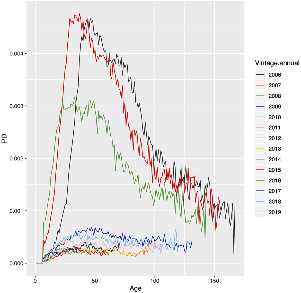
Figure 1. Plot of the annual vintage data for conditional probability of default for Fannie Mae and Freddie Mac 30-year prime conforming mortgage data.
A 10% sample was taken from the $2 trillion in available mortgage data for purposes of model estimation and validation. This created a dataset with 622,452 unique loans of which 4,346 defaulted for a lifetime default rate of 0.7%. This data included vintages from January 1999 through November 2019 with performance data from January 2017 through December 2019 with FICO scores between 660 and 780.
4. Methods
All of the models compared use a panel data approach. Specifically, we create panel behavioral models:
• Multihorizon survival
• Neural network with panel data
• Neural network with APC lifecycle and environment inputs
• Stochastic gradient boosted trees (SGBT) with penal data
• SBGT with APC lifecycle and environment inputs
Each of these methods build one model for each forecast horizon, following the approach of multihorizon survival models for capturing the nonlinear forecast response to delinquency status. In theory, most machine learning methods should be compatible with APC inputs and a multihorizon structure, but only NN and SGBT were found to have libraries that accepted the fixed offsets necessary for this approach.
4.1. Age-Period-Cohort models
Age-Period-Cohort models originated as an estimation method for extracting information from Lexis diagrams [50, 51]. Cohort models were adopted in sociology and epidemiology in the 1960s [52] and their statistical foundations were studied in depth in the decades thereafter [53, 54]. The concepts were independently discovered in application to loan portfolio stress testing [55] where it is commonly referred to as vintage analysis, and APC models or similar variants are now widely used globally for stress testing and lifetime performance forecasting.
Several of the methods described above will use inputs from an initial Age-Period-Cohort (APC) analysis. APC models describe the risk of default at each observation period through the life of the loan as functions of the age a of the loan, the calendar date t, and the vintage date v. These functions can be spline approximations, non-parametric, or other forms. For this analysis, a Bayesian APC algorithm was employed to estimate these functions non-parametrically [36]. Using non-parametric estimations of these functions allows them to capture detailed nonlinear structures even when no cause can be assigned. Leaving the use of explanatory factors to a later stage of the analysis is a primary source of effectiveness for these algortihms.
Because a = t−v, a model specification error exists if no constraints are imposed [56, 57]. In applications to credit risk analysis, the following representation is common.
where b0 is the intercept, b1 and b2 are the linear coefficients for a and v, and F′(a), G′(v), and H′(t) are the nonlinear functions that have zero mean and no linear component. For explanation, these are usually combined as
where F(a) is called the lifecycle measuring the timing of losses through the life of the loan, G(v) is the vintage function measuring credit risk by vintage, and H(t) is the environment function measuring the net impact from the environment (primarily economic conditions). Intuitively, the specification error has been resolved by forcing the environment function to have zero mean. This is most appropriate with long time histories spanning more than one recession, because it is consistent with assuming that a through-the-cycle PD exists. Over spans of just a few years, the macroeconomic environment usually has a net trend of expansion or contraction, so an assumption os zero trend would be unlikely to hold. The misallocation of trends over short time spans is assumed to be a primary cause of the instability in traditional cross-sectional scores that is observed in the model results here, even when the testing environment has only a mild trend.
The primary advantage of APC models is the ability to separate age, vintage, and time effects, so the credit risk function captures the full amount of credit quality variation, but is cleaned of impacts from the macroeconomic environment and normalized for differences in the age of the loans. This analysis can be segmented, as is commonly done by score and term in order to capture corresponding shifts in the lifecycle. In this case, the data was selected so that only one lifecycle is necessary. No state or MSA segmentation was performed for the environment function, which is equivalent to assuming that the loan mix by state geography is relatively constant. This is a reasonable assumption for the Fannie Mae and Freddie Mac data.
4.2. Multihorizon survival model
Traditional credit scores [58, 59] assume a fixed outcome interval, like the first 36 months of a loan, to observe whether any defaults occur during this time, and then attempt to model this via logistic regression. Logistic regression credit scores are ubiquitous for rank-ordering loan risk, but the use of a fixed observation window without indication of when a default might have occurred within that window prevents such models from being integrated effectively with macroeconomic factors, cash flow modeling, and a number of other applications.
A panel logistic regression model can optimize the scoring coefficients over multiple future forecast horizons, possibly with time-varying independent variables. The dependent variable can be taken as a specific number of months into the future h from the last observation date t0.
where the cj are the n estimated coefficients for the scoring factors sij(t0) for account i. The set of scoring factors s are chosen to optimize the Akaike Information Criterion (AIC). In a regression model, some of the scoring variables may be binned to capture nonlinearities. All of the well-known aspects of a scoring model are preserved, except that the data has one observation for each account each month until it defaults or is censored from early pay-off or reaching the end of the data.
Discrete time survival models (DTSM) [60, 61] are a form of panel logistic regression where information on the loan age and macroeconomic environment are added to the regression inputs. Some researchers have included these as dummy variables for each age and calendar date or include parameters for an age function and macroeconomic variables so that the hazard function and macroeconomic sensitivities are estimated concurrently with the scoring factors.
To avoid multicolinearity problems, we prefer to use a multihorizon survival modeling approach where the lifecycle and environment from an APC model as fixed inputs and estimate only the coefficients for the scoring factors. Equation 6 shows this structure. From a regression perspective, F(a) and H(t) are inputs with coefficients equal to 1. In the language of most logistic regression implementations, this is a fixed offset. If the target variable were continuous, we could compute the residuals relative to the APC inputs and model that with only scoring factors. Having a binary target variable requires the use of an offset among the input variables.
Delinquency is obviously correlated to macroeconomic variables such as unemployment, but with this approach, maximum explanatory power is given to macroeconomic factors and account-specific measures such as delinquency are used only to explain the account-level distribution centered about the portfolio trends. A separate model is estimated for each forecast horizon. Comparing the coefficients for the first six horizons shows that they can change rapidly because of the complicated relationship between delinquency at t0 and future defaults. However, the information value of delinquency decays rapidly, so by horizon 12 the coefficients cj will usually have reached their saturation values with delinquency being less important. Of course, this can be tested for specific problems. For the current analysis, all models are estimated through horizon 12.
In order to capture potential nonlinear structure between some of the scoring variables and probability of default, CLTV, LTV, and DTI were binned with separate coefficients estimated for each bin. A backward stepwise regression process was used to select the best set of predictive variables to optimize AIC. This modeling was performed separately for each forecast horizon, h∈[1, 12].
4.3. Artificial neural network
Using artificial neural networks (NN) for credit risk forecasting has been the subject of numerous publications [21, 22, 62]. The problem design is similar to creating a logistic regression credit score, but with the network allowing for non-linearity and interaction effects that would need to be discovered manually and encoded into the inputs of a regression model.
Data for defaults on conforming mortgages does not include the kind of nonlinear alternate data where neural networks are most compelling. The application to mortgage data is just to demonstrate the technique, rather than trying to perform a competition between methods. Because the inputs are traditional financial and loan application information, unintended ethical bias would not be a problem regardless of the amount of nonlinear complexity of the NN.
In order to accelerate the training of the neural network, all continuous variables were standardized to mean = 0, deviation = 1. No binned variables were included, because the NN should be able to learn any nonlinear structure required for incorporating these variables. Binning with a corresponding coefficient estimated for each bin is useful with linear regression models that cannot otherwise capture non-linear structure.
The neural network architecture was simpler than applications involving alternate data. The network had an input layer, 5 fully connected layers with softplus activation functions, and a sigmoid output node. Softplus is less efficient and some argue less interpretable than ReLu activation functions, but it had better convergence performance in this context. The target was the same binary indicator of default within 24 months as used in the logistic regression model with a binary cross-entropy loss function. This architecture was the result of running a small set of tests to explore deeper or wider designs. Some architecture optimization is desirable for best performance, but extensive testing leads to overfitting the test data.
Neural networks do not estimate well when defaults comprise only 0.2% of the training data. Previous research has shown that at least a 4:1 or 3:1 ratio is needed for proper network estimation [63, 64]. In this case, a random undersampling approach was used where all default accounts were included and four times as many non-default accounts were randomly sampled from the dataset. More advanced data sampling methods have been developed, such as Synthetic Minority Over-sampling Technique (SMOTE) [65], Adaptive Synthetic Sampling (ADASYN) [66], or Active Learning [67]. Although these methods may leverage the training data better, they can distort the relationship to the APC inputs. Random sampling allows us to develop easily rebalance the model forecasts to match the default probability distribution of the original training dataset.
Equation 7 provides a closed form solution for rebalancing the predictions, derived using Bayes' Theorem [68].
where p0 and p1 are a priori probabilities for the original data and and are a priori probabilities for the balanced dataset, y is the neural network forecast with the balanced dataset, and y′ is the forecast for the original dataset. The same could be achieved numerically by performing a logistic regression on the NN forecasts to estimate the needed scaling factor for the original dataset. This simple numerical approach works in our case with fixed APC inputs, but other methods have been proposed in general [69].
4.4. NN + APC
In order to combine neural networks with APC lifecycle and environment functions, these inputs should not be included as any other scoring factors, because then we would lose the separability assumption from APC models that resolved the multicolinearity problem. Instead, we created a custom network design as shown in Figure 2 where the APC inputs O(a, t) = F(a)+H(t) in units of log-odds of default are passed to the final node as an offset without modification. The neural network is used only as a replacement for the credit risk component of an APC model, effectively modeling the account-level residuals around the long-term trends of lifecycle and environment.

Figure 2. A neural network architecture designed to take fixed inputs of lifecycle F(a) and enviornent H(t) from an APC decomposition.
This structure was first proposed by Breeden and Leonova [10]. In a behavior scoring context, a separate neural network was estimated for each forecast horizon. In principle, a single network could be created with one output node for each forecast horizon and one offset connected to each output node. However, the approach of having a collection of neural networks was used in order to parallelize the computations.
For proper estimation, the dataset still requires balancing, but Equation 7 is no longer applicable when an offset is supplied to the network. Instead, the input offset needs to be adjusted with an additive constant for any change in default probabilities due to rebalancing. For this study, revised offset, O′ was estimated as a constant added to the original offset in order to incorporate the sample bias. When the network produces forecasts, the original offset O(a, t) is used without the rebalancing adjustment factor. As with the plain NN, the dataset for model estimation under-sampled the loans that never default in order to achieve a 4:1 ratio with loans that eventually will default. Model training was performed on 80% of this balanced dataset and cross-validation on 20% to determine the stopping point.
4.5. Stochastic gradient boosted trees
Decision trees have been used for decades in credit risk modeling [70, 71]. The multidimensional space described by the scoring variables is split by hyperplanes to separate good from bad accounts. In the current research, we created regression trees where regression models are constructed within each resulting hypercube, as in CART [72].
Stochastic gradient boosted trees [73, 74] are essentially an ensemble modeling approach. The algorithm starts with a base learner, which can be any starting model, but is usually implemented as an initial tree. The prediction residuals from the base learner are used to weight the data, more weight on the most poorly predicted points, so that the next tree is built to be an additive refinement of all previous trees. Trees are added to the ensemble until no significant improvement is obtained on a cross-validation set.
Using SGBT models also involves architecture decisions. After experimentation, the optimal depth (number of levels of the tree) was found to be three. This is consistent with the finding that the optimal neural network architecture had only a few layers. The input data does not contain the complexity of analyzing a corporate financial statement or extracting sentiment from call center logs, so the model is correspondingly simple, The number of trees in the ensemble was also kept relatively small in order to avoid overfitting.
The SGBT models were constructed on the same panel data as previous models with one model created for each forecast horizon. In total 80% of the data was used for model estimation and 20% for cross-validation to identify the stopping point.
4.6. SGBT + APC
Because SGBT algorithms are sequential refinements to a base learner, making the base learner an Age-Period-Cohort model would be a natural extension. However, by providing the APC inputs as a fixed offset, all trees are adjusted so that none try to alter the APC structure. Some implementations of stochastic gradient boosted trees allow for the same kind of fixed inputs as logistic regression. Again defining the offset, O(a, t) = F(a)+H(t), as a fixed input allows us to create an SGBT credit risk panel model that is centered around the long-term trends of lifecycle and environment. For proper calibration, the offset O(a, t) must be in units of log-odds of default, not probability of default. The offset is used at the point where the regression trees are constructed in order to normalize for account age and environmental impacts.
The input variables and sampling for cross-validation were the same as the SGBT model without APC inputs. One model was created for each of twelve forecast horizons.
5. Results
All of the data was used to perform the APC decomposition. The resulting lifecycle, environment, and vintage functions are shown in Figure 3 for probability of default and in Figure 4 for probability of prepayment. These estimates are monthly rates conditional on the account being active in the previous month. The PD lifecycle increases vs. the age of the account because of the selection effect where better loans are likely to refinance earlier. The environment function for PD clearly shows the 2001 and 2009 recessions along with annual seasonality. The vintage function for PD shows the poor quality loans booked prior to the 2009 recession and steadily increasing risk through the end of the data.
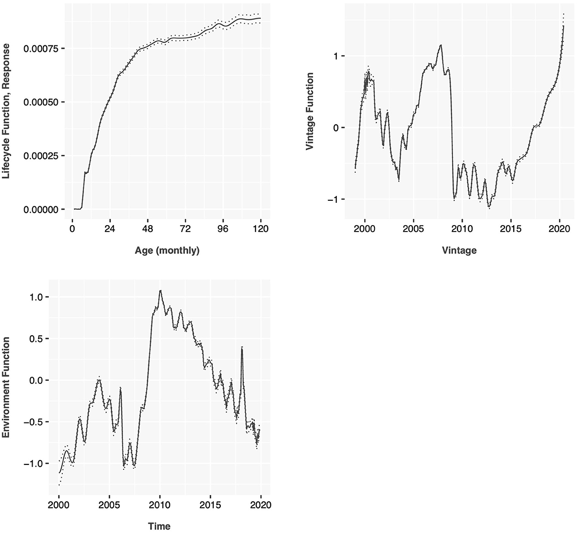
Figure 3. Age-period-cohort decomposition of probability of default for 30-year prime conforming mortgage data.

Figure 4. Age-period-cohort decomposition of probability of prepayment for 30-year prime conforming mortgage data.
The environment and vintage functions for the probability of prepayment, Figure 4 show more volatile structure, because they are dependent on changes in mortgage interest rates.
For development of account-level models, identical samples were used across the model types. A 20% sample was used for model training. The remaining 80% was used for out-of-sample testing during the same time period. A separate data selection was used for out-of-time testing.
For accounts less than 6 months old, an origination score was developed using a discrete time survival model approach with APC inputs of lifecycle and environment. Table 1 shows the coefficients of this model. This table is included primarily as a representation of the kinds of factors that were found to be useful in the modeling.
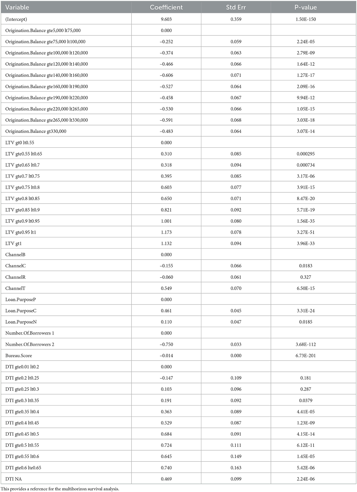
Table 1. Coefficients for a discrete time survival model (no behavioral factors and no dependence upon forecast horizon).
From this example output, the usual factors show up as important. Bureau score is the most important and has a reliably linear relationship with log-odds of default. Loan-to-value (LTV) has a more nonlinear structure, probably due to the pricing changes that occur at certain threshold values. Therefore LTV and debt-to-income (DTI) are both binned prior to modeling in order to allow the regression model to capture some of the non-linearities. Origination balance was found to be predictive, probably because of the implied difference in risk between small loans and jumbo loans, although this might be more predictive in combination with other variables. Most of the p-values are very significant because of the large amount of data available. Some individual coefficients within a set of coefficients for a binned variable may be insignificant, but this just indicates that it is close to the reference level. Individual bins need not be removed from the model. Rather, if none of the coefficients for a binned variable were significant, then the entire variable might be removed.
When delinquency is added to the model, a multihorizon survival model is estimated. Figure 5 shows how the coefficients for delinquency change versus forecast horizon. For the first six months, delinquency is the dominant factor in the model, but beyond six months, the other factors seen in the origination score become more important.
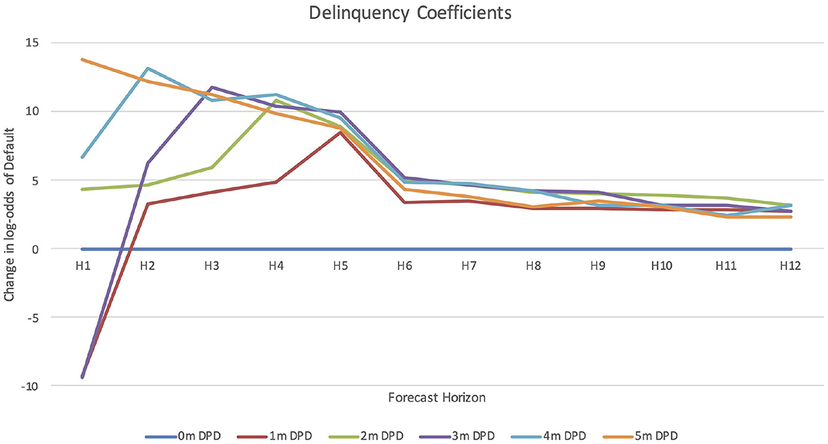
Figure 5. A visualization of the coefficients estimated by forecast horizon for delinquency, binned by number of payments missed.
The same factors were provided as inputs to the stochastic gradient boosted trees and neural network models. These models were estimated separately for each forecast horizon, as was done with the multihorizon survival model. We also create two versions of each, one with APC inputs and one without. Table 2 shows the relative influence of factors in the stochastic gradient boosted trees model with APC inputs included via an offset.
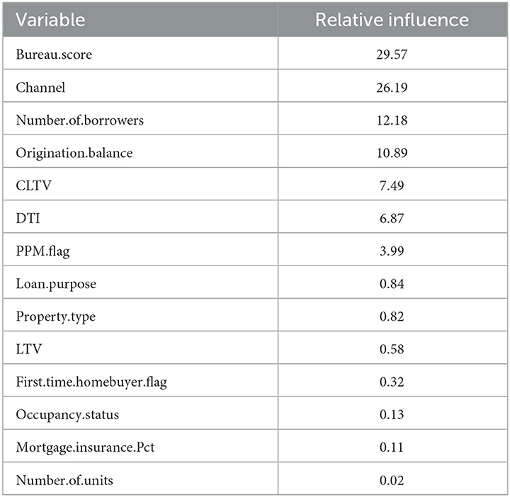
Table 2. Input factor sensitivities for the stochastic gradient boosted tree model with APC inputs for lifecycle and environment (SGBT+APC).
All of the panel models created were designed to predict the probability of default conditional on the account being active in the previous month. In order to run a long-range forecast, we must simultaneously predict the probability of prepayment each month. This could be done with a series of scores comparable to the PD scores described above. However, for purposes of simplifying the tests, only the vintage-level APC models of probability of prepayment were employed to predict the monthly probability of being active. The final test results therefore translate the conditional PDs to unconditional PDs using the pre-payment probabilities.
Table 3 collects the in-sample, out-of-sample, and out-of-time test results for all of the models. The full-period tests mean that a snapshot of accounts was taken in the month prior to the test period and the forecast was run for the full period. Annual tests mean that a new snapshot was taken each year and a series of 12-month tests was conducted with the combined results reported.
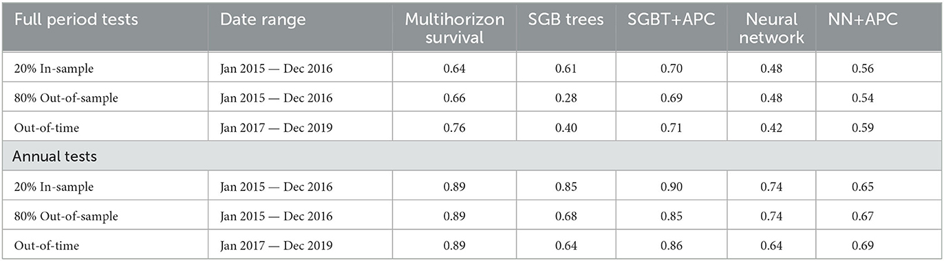
Table 3. Test results comparing the Gini coefficient for the models built on 30-year conforming prime mortgage data.
In most credit scoring competitions, SGBT has been a winning approach. Recent research by Grinsztajn et al. [75] suggests that tree-based models will perform better than neural networks for tabular data structures where neighboring input factors may have no ordering or continuity. Neural networks have been found to excel in sound and image processing applications where the inputs are neighboring pixels in an image or sequential points in the time sampling. Although effort was put into choosing good designs for the neural networks and SGB Trees, they were not optimized so much that we would want to declare a winner between them.
The most important result is that when looking at the SGB Trees and Neural Networks, even accepting a certain amount of testing noise, the models degrade out-of-sample and out-of-time. The neural network degrades less, but it may also have been less overfit in-sample to begin with. For the models with APC inputs: multihorizon survival, SGBT+APC, and NN+APC, no out-of-sample or out-of-time performance degradation is observed. In fact, in all three cases the performance ticked up slightly out-of-time, but that is not easily explainable as anything more than testing noise. One primary goal for providing APC lifecycle and environment as fixed inputs is that the machine learning models focus just on modeling the account distribution about the APC time-varying mean so that the scores generalize better out-of-sample and out-of-time. That appears to be happing.
With this test design, questions about information leakage could arise. The theory behind APC models asserts that the lifecycle, environment, and vintage functions are separable, so using all of the data to estimate the lifecycle does not influence estimation of the panel credit score. Looking out-of-time, the test is using the actual APC environment function to set the mean of the distribution. This is definitely future information, but it will not impact the rank ordering of the account level scoring model. By focusing on a rank ordering statistic (Gini), we are separating the question of how well the future environment can be forecasted from the quality of the account-level discrimination.
Note that the economy was relatively benign during the train and test periods. If a recession had been present in the out-of-time test period, the scoring approaches would be expected to perform much worse whereas the macroeconomic scenarios provided via the APC inputs could continue to guide the forecasts. The models were not explicitly tested on their accuracy in predicting total loss rates, because the models without APC inputs simply could not do so. The aggregate forecast accuracy for the multihorizon survival, SGBT+APC, and NN+APC will depend primarily on the accuracy of the APC model.
6. Conclusion
The purpose of this research was to extend logistic regression insights on long-range forecasting and stress testing to commonly used machine learning methods. Multihorizon survival models have previously been shown to extend logistic regression scoring models for use in account-level lifetime forecasting, stress testing, and volatility analysis. The key to this advancement was adopting a panel data structure and taking age-period-cohort inputs for lifecycle and environment as fixed inputs to the model training. This was found to enhance out-of-sample and out-of-time stability and enable scenario-based forecasting.
Machine learning models have rarely been shown in use with panel-structured data in credit risk modeling, probably because the use case was not compelling. However, by adopting a panel data structure and taking the same APC lifecycle and environment offsets as fixed inputs, we replicated the performance enhancement and gain of function that was seen previously for logistic regression models. Implementations of stochastic gradient boosted trees were found which accepted fixed inputs when regression trees are used. Neural network implementations do not provide this architecture by default, but we were able to replicate it with some simple design changes. Support vector machines, which have also been tested for use in credit scoring, have not been found to support the incorporation of fixed inputs.
Out-of-sample and out-of-time degradation of model performance has been one of the dominant problems in machine learning. Several architectural refinements have been introduced that may reduce overfitting for machine learning models, and those methods may be combined with the technique developed here. However, even with no such refinements, our technique of incorporating APC lifecycle and environment inputs dramatically stabilizes the use of machine learning methods. This would seem to demonstrate that much of the overfitting that has been occurring in machine learning model estimation when applied to credit scoring is an attempt by the algorithm to explain short-term trends that are better explained as a piece of a longer trend due to the product lifecycles or macroeconomic environment. Using pre-trained APC inputs performs better than simply adding account age fixed effects or macroeconomic factors, because correlations to delinquency and other scoring factors could destabilize the model whereas APC analysis has explicit controls to separate these effects.
This approach allows the analyst to leverage long histories of limited data for the APC analysis and then incorporate the APC components into machine learning models on short data sets. Combining the analysis of long, thin datasets with the analysis of short, wide (many input variables) datasets is unique and allows for these long trends to be explained with macroeconomic factors. When only a short time history is available, the same approach applies and the score rank ordering can be enhanced relative to traditional methods, but extrapolating the environment function becomes more challenging. These are the limitations of any stress test model built upon short histories, and the literature on using APC models for forecasting should be reviewed by the analyst before extending the use of the models from simple scoring to cash flow modeling, lifetime loss and yield estimates, capital calculations, etc.
With enough history so that the preceding caveat is resolved, a key advantage of any panel data score is that the monthly forecasts can be summed over any forecast horizon. That means that the same model that is used for account management with a 24-month horizon can be used for Basel II with a through-the-cycle environment function and a 12-month forecast horizon. Similarly, the same model can be used for all stages of estimating IFRS 9 loss reserves where both 12-month and lifetime forecasts are required. This flexibility is a significant business advantage in terms of development, validation, and deployment costs. Questions around using machine learning models for regulatory purposes are left to another discussion.
Although the language and example applications of this article are focused on lending, the methods are generic. These methods have already been tested for predicting the value of fine wines [76]. In any field where vintage data can be found, these methods can be used to improve account-level, item-level, or consumer-level analysis.
Merging vintage analysis with the most popular machine learning techniques means that we can integrate account-level machine learning modeling with portfolio forecasting. A single model backbone can support credit risk modeling needs across a wide range of business functions without introducing compromises.
Data availability statement
Publicly available datasets were analyzed in this study. This data can be found here: https://www.freddiemac.com/research/datasets/sf-loanlevel-dataset, https://capitalmarkets.fanniemae.com/credit-risk-transfer/single-family-credit-risk-transfer/fannie-mae-single-family-loan-performance-data.
Author contributions
JB and YL worked together on developing the algorithms and tests. JB provided the conceptual guidance and wrote the article. Both authors contributed to the article and approved the submitted version.
Conflict of interest
JB and YL are employed by Deep Future Analytics LLC.
Publisher's note
All claims expressed in this article are solely those of the authors and do not necessarily represent those of their affiliated organizations, or those of the publisher, the editors and the reviewers. Any product that may be evaluated in this article, or claim that may be made by its manufacturer, is not guaranteed or endorsed by the publisher.
References
1. Turkyilmaz CA, Erdem S, Uslu A. The effects of personality traits and website quality on online impulse buying. Procedia-Soc Behav Sci. (2015) 175:98–105. doi: 10.1016/j.sbspro.2015.01.1179
2. Tan T, Bhattacharya P, Phan T. Credit-worthiness prediction in microfinance using mobile data: a spatio-network approach. In: Thirty Seventh International Conference on Information Systems, Dublin. (2016).
3. Netzer O, Lemaire A, Herzenstein M. When words sweat: Identifying signals for loan default in the text of loan applications. J Market Res. (2019) 56:960–80. doi: 10.1177/0022243719852959
4. Djeundje VB, Crook J, Calabrese R, Hamid M. Enhancing credit scoring with alternative data. Expert Syst Appl. (2021) 163:113766. doi: 10.1016/j.eswa.2020.113766
5. Wei Y, Yildirim P, Van den Bulte C, Dellarocas C. Credit scoring with social network data. Market Sci. (2016) 35:234–58. doi: 10.1287/mksc.2015.0949
7. Therneau TM, Grambsch PM. Modeling Survival Data: Extending the Cox Model. New York: Springer-Verlag. (2000). doi: 10.1007/978-1-4757-3294-8
8. Singer JD, Willett JB. It's about time: Using discrete-time survival analysis to study duration and the timing of events. J Educ Statist. (1993) 18:155–95. doi: 10.3102/10769986018002155
9. Muthén B, Masyn K. Discrete-time survival mixture analysis. J Educ Behav Statist. (2005) 30:27–58. doi: 10.3102/10769986030001027
10. Breeden JL, Leonova E. When Big Data Isn't Enough: Solving the long-range forecasting problem in supervised learning. In: 2019 International Conference on Modeling, Simulation, Optimization and Numerical Techniques (SMONT 2019). Atlantis Press (2019). p. 229–232. doi: 10.2991/smont-19.2019.51
11. Breeden JL, Crook J. Multihorizon discrete time survival models. J Oper Res Soc. (2020) 73:56–69. doi: 10.1080/01605682.2020.1777907
12. Galindo J, Tamayo P. Credit risk assessment using statistical and machine learning: basic methodology and risk modeling applications. Comput Econ. (2000) 15:107–43.
13. Bhatore S, Mohan L, Reddy YR. Machine learning techniques for credit risk evaluation: a systematic literature review. J Bank Finan Technol. (2020) 4:111–38. doi: 10.1007/s42786-020-00020-3
14. Breeden J. A survey of machine learning in credit risk. J Credit Risk. (2021) 17:342. doi: 10.21314/JCR.2021.008
15. Friedman JH. Greedy function approximation: a gradient boosting machine. Ann Stat. (2001) 29:1189–232. doi: 10.1214/aos/1013203451
16. Friedman JH. Stochastic gradient boosting. Comput Stat Data Anal. (2002) 38:367–78. doi: 10.1016/S0167-9473(01)00065-2
17. Schapire RE. The boosting approach to machine learning: An overview. In: Nonlinear estimation and classification. Springer (2003). p. 149–171. doi: 10.1007/978-0-387-21579-2_9
18. Schapire RE, Freund Y. Boosting: Foundations and Algorithms. London: MIT Press. (2013). doi: 10.7551/mitpress/8291.001.0001
19. Chen T, Guestrin C. Xgboost: A scalable tree boosting system. In: Proceedings of the 22nd ACM SIGKDD International Conference on Knowledge Discovery and Data Mining. (2016). p. 785–794. doi: 10.1145/2939672.2939785
20. Piramuthu S. Financial credit-risk evaluation with neural and neurofuzzy systems. Eur J Oper Res. (1999) 112:310–21. doi: 10.1016/S0377-2217(97)00398-6
21. Angelini E, Di Tollo G, Roli A, A. neural network approach for credit risk evaluation. Quart Rev Econ Finan. (2008) 48:733–55. doi: 10.1016/j.qref.2007.04.001
22. Khashman A. Neural networks for credit risk evaluation: Investigation of different neural models and learning schemes. Expert Syst Appl. (2010) 37:6233–9. doi: 10.1016/j.eswa.2010.02.101
23. Baesens B, Setiono R, Mues C, Vanthienen J. Using neural network rule extraction and decision tables for credit-risk evaluation. Manage Sci. (2003) 49:312–29. doi: 10.1287/mnsc.49.3.312.12739
24. Schebesch KB, Stecking R. Support vector machines for classifying and describing credit applicants: detecting typical and critical regions. J Oper Res Soc. (2005) 56:1082–8. doi: 10.1057/palgrave.jors.2602023
25. Huang CL, Chen MC, Wang CJ. Credit scoring with a data mining approach based on support vector machines. Expert Syst Appl. (2007) 33:847–56. doi: 10.1016/j.eswa.2006.07.007
26. Malekipirbazari M, Aksakalli V. Risk assessment in social lending via random forests. Expert Syst Appl. (2015) 42:4621–31. doi: 10.1016/j.eswa.2015.02.001
27. Ho TK. The random subspace method for constructing decision forests. IEEE Trans Pattern Anal Mach Intell. (1998) 20:832–44. doi: 10.1109/34.709601
28. Ishwaran H, Kogalur UB, Blackstone EH, Lauer MS. Random survival forests. Ann Appl Stat. (2008) 2:841–60. doi: 10.1214/08-AOAS169
29. Hothorn T. Bühlmann P, Dudoit S, Molinaro A, Van Der Laan MJ. Survival ensembles. Biostatistics. (2006) 7:355–73. doi: 10.1093/biostatistics/kxj011
30. Wang P, Li Y, Reddy CK. Machine learning for survival analysis: A survey. ACM Comput Surv. (2019) 51:1–36. doi: 10.1145/3214306
31. Mani D, Drew J, Betz A, Datta P. Statistics and data mining techniques for lifetime value modeling. In: Proceedings of the fifth ACM SIGKDD International Conference on Knowledge Discovery and Data Mining. (1999). p. 94–103. doi: 10.1145/312129.312205
32. Brown SF, Branford AJ, Moran W. On the use of artificial neural networks for the analysis of survival data. IEEE Trans Neural Netw. (1997) 8:1071–7. doi: 10.1109/72.623209
34. Ohno-Machado L. Sequential use of neural networks for survival prediction in AIDS. In: Proceedings of the AMIA Annual Fall Symposium. American Medical Informatics Association (1996). p. 170.
35. Hess KR, Serachitopol DM, Brown BW. Hazard function estimators: a simulation study. Stat Med. (1999) 18:3075–88. doi: 10.1002/(SICI)1097-0258(19991130)18:22<3075::AID-SIM244>3.0.CO;2-6
36. Schmid V, Held L. Bayesian Age-Period-Cohort Modeling and Prediction - BAMP. J Statist Softw. (2007) 21:1–15. doi: 10.18637/jss.v021.i08
37. Faraggi D, Simon R, A. neural network model for survival data. Stat Med. (1995) 14:73–82. doi: 10.1002/sim.4780140108
38. Katzman JL, Shaham U, Cloninger A, Bates J, Jiang T, Kluger Y. DeepSurv: personalized treatment recommender system using a Cox proportional hazards deep neural network. BMC Med Res Methodol. (2018) 18:1–12. doi: 10.1186/s12874-018-0482-1
39. Chen Y, Jia Z, Mercola D, Xie X. A gradient boosting algorithm for survival analysis via direct optimization of concordance index. Comput Mathem Methods Med. (2013) 2013:873595. doi: 10.1155/2013/873595
40. Khajehpiri B, Moghaddam HA, Forouzanfar M, Lashgari R, Ramos-Cejudo J, Osorio RS, et al. Survival analysis in cognitively normal subjects and in patients with mild cognitive impairment using a proportional hazards model with extreme gradient boosting regression. J Alzheimer's Dis. (2022) 85:837–50. doi: 10.3233/JAD-215266
41. Banerjee R, Canals-Cerdaá JJ. Credit risk analysis of credit card portfolios under economic stress conditions. Federal Reserve Bank of Philadelphia, Research Department (2012). doi: 10.21799/frbp.wp.2012.18
42. Bellotti A, Crook J. Forecasting and stress testing credit card default using dynamic models. Int J Forecast. (2013) 29:563–74. doi: 10.1016/j.ijforecast.2013.04.003
43. Breeden JL, Thomas LC, McDonald III J. Stress Testing Retail Loan Portfolios with Dual-time Dynamics. J Risk Model Valid. (2008) 2:43–62. doi: 10.21314/JRMV.2008.033
44. Breeden JL, Leonova E, Bellotti A. Instabilities using Cox PH for forecasting or stress testing loan portfolios. (2019).
45. Sargent DJ, A. flexible approach to time-varying coefficients in the Cox regression setting. Lifetime Data Anal. (1997) 3:13.
46. Tian L, Zucker D, Wei L. On the Cox model with time-varying regression coefficients. J Am Stat Assoc. (2005) 100:172–83. doi: 10.1198/016214504000000845
47. Djeundje VB, Crook J. Dynamic survival models with varying coefficients for credit risks. Eur J Oper Res. (2019) 275:319–33. doi: 10.1016/j.ejor.2018.11.029
48. Medina-Olivares V, Calabrese R, Crook J, Lindgren F. Joint models for longitudinal and discrete survival data in credit scoring. Eur J Oper Res. (2023) 307:1457–73. doi: 10.1016/j.ejor.2022.10.022
49. Bocchio C, Crook J, Andreeva G. The impact of macroeconomic scenarios on recurrent delinquency: A stress testing framework of multi-state models for mortgages. Int J Forecast. (2022) in press. doi: 10.1016/j.ijforecast.2022.08.005
50. Keiding N. Statistical inference in the Lexis diagram. Phys Eng Sci. (1990) 332:487–509. doi: 10.1098/rsta.1990.0128
51. Carstensen B. Age-period-cohort models for the Lexis diagram. Stat Med. (2007) 26:3018–45. doi: 10.1002/sim.2764
52. Ryder NB. The Cohort as a Concept in the Study of Social Change. Am Sociol Rev. (1965) 30:843–61. doi: 10.2307/2090964
53. Holford TR. The estimation of age, period and cohort effects for vital rates. Biometrics. (1983) 39:311–24. doi: 10.2307/2531004
54. Mason WM, Fienberg S. Cohort analysis in social research: beyond the identification problem. Springer. (1985). doi: 10.1007/978-1-4613-8536-3
55. Breeden JL. Modeling data with multiple time dimensions. Comput Stat Data Analy. (2007) 51:4761–85. doi: 10.1016/j.csda.2007.01.023
56. Fu W. A Practical Guide to Age-Period-Cohort Analysis: The Identification Problem and Beyond. Chapman and Hall/CRC. (2018). doi: 10.1201/9781315117874
57. Breeden JL, Thomas LC. Solutions to specification errors in stress testing models. J Oper Res Soc. (2016) 67:830–40. doi: 10.1057/jors.2015.97
58. Thomas L, Crook J, Edelman D. Credit Scoring and Its Applications. Bangkok: SIAM. (2017). doi: 10.1137/1.9781611974560
59. Anderson R. Credit Intelligence & Modelling: Many Paths through the Forest. Oxford: Oxford University press (2019).
60. Stepanova M, Thomas L. Survival analysis methods for personal loan data. Oper Res. (2002) 50:277–89. doi: 10.1287/opre.50.2.277.426
61. De Leonardis D, Rocci R. Assessing the default risk by means of a discrete-time survival analysis approach. Appl Stoch Models Bus Ind. (2008) 24:291–306. doi: 10.1002/asmb.705
62. Desai VS, Crook JN, Overstreet Jr GA, A. comparison of neural networks and linear scoring models in the credit union environment. Eur J Oper Res. (1996) 95:24–37. doi: 10.1016/0377-2217(95)00246-4
63. Laurikkala J. Improving identification of difficult small classes by balancing class distribution. In: Artificial Intelligence in Medicine: 8th Conference on Artificial Intelligence in Medicine in Europe, AIME 2001. Cascais, Portugal: Springer (2001). p. 63–66. doi: 10.1007/3-540-48229-6_9
64. Sundarkumar GG, Ravi V, A. novel hybrid undersampling method for mining unbalanced datasets in banking and insurance. Eng Appl Artif Intell. (2015) 37:368–77. doi: 10.1016/j.engappai.2014.09.019
65. Chawla NV, Bowyer KW, Hall LO, Kegelmeyer WP. SMOTE synthetic minority over-sampling technique. J Artif Intell Res. (2002) 16:321–57. doi: 10.1613/jair.953
66. He H, Bai Y, Garcia EA, Li S. ADASYN: Adaptive synthetic sampling approach for imbalanced learning. In: 2008 IEEE International Joint Conference on Neural Networks (IEEE world congress on computational intelligence). IEEE (2008). p. 1322–8.
67. Aggarwal U, Popescu A, Hudelot C. Active learning for imbalanced datasets. In: Proceedings of the IEEE/CVF Winter Conference on Applications of Computer Vision. (2020). p. 1428–37. doi: 10.1109/WACV45572.2020.9093475
68. Dal Pozzolo A, Caelen O, Johnson RA, Bontempi G. Calibrating probability with undersampling for unbalanced classification. In: 2015 IEEE Symposium Series on Computational Intelligence. IEEE (2015). p. 159–66. doi: 10.1109/SSCI.2015.33
69. Wallace BC, Dahabreh IJ. Improving class probability estimates for imbalanced data. Knowl Inf Syst. (2014) 41:33–52. doi: 10.1007/s10115-013-0670-6
71. Ali K, Pazzani M. Error reduction through learning multiple descriptions. Mach Learn. (1996) 24:172–202. doi: 10.1007/BF00058611
72. Breiman L, Friedman J, Stone CJ, Olshen RA. Classification and regression trees. New York: CRC Press. (1984).
73. Chang YC, Chang KH, Wu GJ. Application of eXtreme gradient boosting trees in the construction of credit risk assessment models for financial institutions. Appl Soft Comput. (2018) 73:914–20. doi: 10.1016/j.asoc.2018.09.029
74. Bastos J. Credit scoring with boosted decision trees. CEMAPRE, School of Economics and Management (ISEG), Technical University of Lisbon; (2007). MPRA Paper No. 8034. Available online at: https://mpra.ub.uni-muenchen.de/8034/ (accessed January 31, 2023).
75. Grinsztajn L, Oyallon E, Varoquaux G. Why do tree-based models still outperform deep learning on tabular data? arXiv preprint arXiv:220708815. (2022).
Keywords: credit scoring, survival models, Age-Period-Cohort, neural networks, stochastic gradient boosted trees
Citation: Breeden JL and Leonova Y (2023) Stabilizing machine learning models with Age-Period-Cohort inputs for scoring and stress testing. Front. Appl. Math. Stat. 9:1195810. doi: 10.3389/fams.2023.1195810
Received: 29 March 2023; Accepted: 23 May 2023;
Published: 08 June 2023.
Edited by:
Raffaella Calabrese, University of Edinburgh, United KingdomReviewed by:
Stefan Lessmann, Humboldt University of Berlin, GermanyWouter Verbeke, KU Leuven, Belgium
Copyright © 2023 Breeden and Leonova. This is an open-access article distributed under the terms of the Creative Commons Attribution License (CC BY). The use, distribution or reproduction in other forums is permitted, provided the original author(s) and the copyright owner(s) are credited and that the original publication in this journal is cited, in accordance with accepted academic practice. No use, distribution or reproduction is permitted which does not comply with these terms.
*Correspondence: Joseph L. Breeden, YnJlZWRlbkBkZWVwZnV0dXJlYW5hbHl0aWNzLmNvbQ==