Bayesian synthetic likelihood for stochastic models with applications in mathematical finance

We present a Bayesian synthetic likelihood method to estimate both the parameters and their uncertainty in systems of stochastic differential equations. Together with novel summary statistics the method provides a generic and model-agnostic estimation procedure and is shown to perform well even for small observational data sets and biased observations of latent processes. Moreover, a strategy for assessing the goodness of the model fit to the observational data is provided. The combination of the aforementioned features differentiates our approach from other well-established estimation methods. We would like to stress the fact that the algorithm is pleasingly parallel and thus well suited for implementation on modern computing hardware. We test and compare the method to maximum likelihood, filtering and transition density estimation methods on a number of practically relevant examples from mathematical finance. Additionally, we analyze how to treat the lack-of-fit in situations where the model is biased due to the necessity of using proxies in place of unobserved volatility.

1. Introduction

Parameter estimation in systems of stochastic differential equations (SDEs) is a crucial task in many practical applications and the ability to quantifying the uncertainty of the parameter estimates is a key feature of modern estimation methods. In mathematical finance, stochastic volatility models are used to describe both the movements of the underlying assets as well as the corresponding latent volatility process. During the last two decades, volatility has become an asset class of its own (see, e.g., [1]), and modeling it using carefully calibrated SDE models is an active research area both in academia and practice. As volatility is not directly observable, one has to rely on volatility proxies in order to calibrate these models under the physical measure which is necessary, e.g., in insurance risk management under the Solvency II framework: For the calculation of available capital, market consistent evaluation of both assets and liabilities given both risk-neutral and real-world stress scenarios is required (cf. [2]). This work is motivated by the necessity of feasible parameter estimation given stock price time series and volatility proxy observation data. For the well-known Heston system of SDEs, both filtering approaches and maximum likelihood estimators have been traditionally used to estimate parameters (see, e.g.,[3–8]). However, the volatility process can not be observed directly and these approaches can be quite sensitive to noise and modeling errors due to the use of volatility proxies. Moreover, filtering approaches require some manual fine tuning and maximum likelihood methods provide merely point estimates without quantifying the inherent uncertainty. On top of that, the computation of the likelihood function is model specific. Therefore a generic model-agnostic estimation procedure with the ability to quantify estimation uncertainty would be desirable. In this work, we introduce such a method which performs well even for comparably small observational data sets and biased indirect observations of the volatility process via proxies. Moreover, we provide a strategy to assess the goodness of the model fit to the data. In order to demonstrate the feasibility of our method, we consider test cases from mathematical finance. We would, however, like to stress once more that the proposed method is generic and may therefore be employed in various fields of application.

SDE systems are commonly written as a sum of a stochastic part and a deterministic evolution model

$\begin{array}{ll}dx=f(x,t;\theta )dt+L(x,t;\theta )w(t),& (1)\end{array}$

where x∈ℝⁿ, f is a drift function, w is an n-dimensional zero-mean white Gaussian process, θ is an unknown parameter vector and the diffusion term L may depend on x, t and θ. A standard method to estimate the parameter vector θ is to approximate the maximum likelihood or the maximum a posteriori (MAP) estimator, conditional on given observational data. Such approaches are well-established in the case of linear SDEs where the transition density p[x(t_k)|x(t_k−1), θ], as a closed-form solution of the Fokker-Planck equation, is available so that the likelihood can be evaluated analytically. This is of course an ideal situation, since in many practically relevant applications the drift function f(·) is non-linear and the diffusion term L depends on the state variables. In that case, the transition density is in general not available in analytical form. To solve such problems, many methods have been implemented. The approach developed in [9] aims to solve the Fokker-Planck equation by an ensemble of simulations that is used to approximate the transition density. likelihood approximation techniques include the simulated maximum likelihood estimation [10] and Hermite expansions [11]. Also filtering approaches have been employed for the estimation of the parameters of such systems, e.g., Kalman or extended Kalman filters, non-linear Gaussian filtering, or ensemble Kalman filters, see for example [12].

In [13], we introduced a distance based approach called correlation integral likelihood (CIL), first proposed by [14], which enables the estimation of both the parameters and their uncertainty, also in the case of non-uniform or sparse data. The focus of this work was on computationally demanding models: We assumed that a sufficiently long time series of data was available, thus allowing the creation of a likelihood for a subset of observations, by subsampling all the available data. The likelihood was computed off-line, and the parameter sampling performed for a subset size data only, thus saving CPU time. In the present work, we study a different way of characterizing the stochastic variability of the state space assuming an in a certain sense complementary setting: Supposing that a sufficient amount of data for a subsampling approach is not available, and that computational limitations do not prevent the use of multiple simulations, we follow the basic idea of synthetic likelihood (SL) by [15], later developed under the title Bayesian synthetic likelihood (BSL) in [16]. In contrast to these works, we employ the idea of [13] using the empirical cumulative distribution function (eCDF) vectors of data as the main way of constructing the statistics. Here the eCDF vectors are based on scalar data directly provided by the SDE systems, unlike the data used in [13]. The likelihood is given by the mean and covariance of the eCDF vectors, which can be empirically estimated. Indeed, the distribution is approximately Gaussian by the Donsker theorem in the case of i.i.d. data, and by more general two sample U-statistic theory in the case of weakly correlated data (see [17]). While the feature vectors may require case-dependent constructions, the approach is otherwise generic. It only requires numerical simulations of the model under consideration, without any further in-depth analysis of the model.

The rest of the paper is structured as follows. Section 2 introduces the BSL method and discusses the details of the implementation with the eCDF as the main summary statistic. Applications of the approach can be found in Section 3. We first apply the method to a toy example, the Ornstein-Uhlenbeck system, where comparisons with analytical solutions and existing filtering methods are also provided. Then, we study the Merton model, where the presence of random jumps renders prediction difficult for filtering methods. Finally, we perform parameter estimation for the Heston model, a common workhorse to model and forecast volatility in the financial industry which is known to reproduce many of the stylized facts observed in real markets. We study parameter estimation for both the case of directly observed volatility and the case of volatility which is indirectly observed via a proxy and we compare our results to an ensemble method introduce in [9].

2. Methods

2.1. Bayesian synthetic likelihood for SDE

The theoretical background of our approach is based on a generalization of the central limit theorem. Instead of the standard mean values we estimate the empirical cumulative distribution function (eCDF) of data. According to the classical Donsker theorem (see [18]), the cumulative distribution function of independent and identically distributed scalar valued data converges toward a Brownian bridge:

Theorem (Donsker, Skorokhod, Kolmogorov). Let F_n be the empirical distribution function of a sequence of independent and identically distributed random variables X₁, X₂, X₃, …X_n which have the distribution function F. Define the centered and scaled version of F_n by

$G_n(x)=\sqrt{n}(F_n(x)-F(x)).$

The sequence of G_n(x), as random elements of the Skorokhod space $\mathcal{D}$, converges in distribution to a Brownian bridge G with zero mean and covariance given by cov(G(s), G(t)) = E[G(s)G(t)] = min(F(s), F(t))−F(s)F(t).

The theorem guarantees asymptotic normality of the empirical distribution function. For further details see [18] or, for more recent presentations, e.g., [19]. In case of a finite-dimensional data the empirical cumulative distribution function is calculated by binning the data. The resulting vector tends to a multi-dimensional Gaussian distribution, with the dimension equal to the number of bins. The examples studied here do not, however, have independent and identically distributed data. Nevertheless, theorems in the U-statistics literature [17, 20] generalize the Donsker theorem for weakly correlated data. In numerical examples the mean and the covariance matrix that define the Gaussian distribution can be estimated by repeatedly computed eCDF vectors. In our examples, we carefully verify the Gaussianity using the χ² test for the set of eCDF vectors, and performing standard normality tests for individual components of the vector. In the present work this likelihood construction is combined with the synthetic likelihood approach.

The synthetic likelihood, or Bayesian synthetic likelihood (BSL), approach aims to approximate the posterior distribution of a set of parameters using simulation-based model fitting. Synthetic likelihood methods are based on the assumption that summary statistics are approximately Gaussian. This allows the construction of a likelihood by estimating the mean and covariance matrix. Similarly to all the likelihood-free methods, this approach is suitable in situations where the likelihood is analytically intractable. The method selects a summary statistic s, which is assumed to store most of the information contained in the observed data y, and is assumed to follow a normal distribution. Depending on the summary statistics, the Gaussianity may be ensured by the central limit theorem, the synthetic likelihood is then asymptotically normal; see [15, 16] for more details.

Given a stochastic model depending on a parameter vector θ and observed data y = (y₁, …, y_N), one aims to estimate the posterior distribution of the model parameters by the Bayes' rule

$\begin{array}{ll}p(\theta |y)~p(y|\theta )p(\theta ).& (2)\end{array}$

In cases where the likelihood is intractable, one constructs a function S:ℝ^N → ℝ^d, which maps the observed data y into a summary statistic vector s_y = S(y) corresponding to the data y. The posterior distribution has the form

$\begin{array}{ll}p(\theta |s_y)~p(s_y|\theta )p(\theta ),& (3)\end{array}$

where p(θ|s_y) should be close to p(θ|y) in distribution. The main issue with this idea is that in many situations where the likelihood on the data is intractable, the same is true for the likelihood on the summary statistic. The idea behind BSL [16] is to use an auxiliary likelihood based on a multivariate normal approximation. Under the assumption that the summary statistic is Gaussian, the estimated synthetic likelihood is of the form $\mathcal{N}(s_y;{\mu }_n(\theta ),{\Sigma }_n(\theta ))$ where μ_n(θ) and Σ_n(θ) are the respective mean and the covariance estimates. In general, the true mean and covariance μ and Σ are unknown and therefore they are estimated by simulating the model n times using the given parameter θ, each time producing a data sample of size N. Based on this synthetic data, the sample mean and sample covariance matrix of the corresponding summary statistic can be calculated. This step can then be embedded in an MCMC algorithm [16]. For each proposed θ, the estimates for μ_n(θ) and Σ_n(θ) are computed, and the proposed candidate is accepted or rejected based on how well s_y fits the constructed likelihood.

The central limit theorem which guarantees asymptotic normality of the synthetic likelihood relies on the strong assumption of multivariate normality of the distribution of the summary statistics. This assumption may not hold in practice, especially when the dimension of the statistics increases. The normality of the summary statistics is naturally guaranteed if the summary is given as a sum of the simulated model values with bounded variance. This may, however, require a high value for the number of repetitions n to ensure empirical normality. Several studies have been carried out to weaken the normality assumption on which the BSL method relies. For example, in [15] the author suggests a transformation of s to achieve multivariate normality, but this may not solve the problem in case of high dimensional summary statistics. The normality assumption is relaxed in [21] by proposing a more flexible density estimator called the extended empirical saddlepoint approximation. The authors of [22] develop a semi-parametric approach to approximate the summary statistics likelihood involving the kernel density estimates for the marginal distributions and a combination of them with a Gaussian copula. In [23], the problem of estimating the parameter posterior is framed as a problem of estimating the ratio between the data generating distribution and the marginal distribution.

In the present work, we avoid such issues by employing the likelihood function based on the eCDF vectors. The Gaussianity is then asymptotically guaranteed by the Donsker theorem—not just an assumption. In our numerical examples we verify the Gaussianity by normality tests, the χ² test for the eCDF vectors, and standard scalar-valued tests for the individual components of the vectors. The so-called ABC methods provide another well-known simulation-based approach for intractable likelihoods, or likelihood-free situations. Our approach differs from them, as we actually do have a well-defined likelihood, that is even normally distributed.

In a nutshell the BSL algorithm proceeds as follows: We simulate the model n times for the proposed parameter value, calculate the eCDF vector of the selected (scalar valued) simulation results, concatenate the vectors (if more than one eCDF is computed) and calculate the mean and covariance of the emerging set of vectors. The synthetic likelihood is thus constructed, and the accept/reject step can be performed as a part of a standard MCMC sampling algorithm.

The basic steps used to find the posterior distribution of the parameters by MCMC sampling are summarized in the Algorithm 1 below. As the likelihood is stochastic, no numerically exact maximum of the likelihood function can exist, but we assume that a robust estimate for the model parameter vector is available, from which to efficiently start the MCMC sampling. In our test cases this is simply the reference value of the model parameter vector used to create the synthetic data, otherwise an optimization step is first performed to match the model to the data. For simplicity we shall call this optimized value the MAP point estimate in the following. However, when fitting a model to real data a bias can be expected, and a test for goodness of fit (or lack of fit) is needed. See the Algorithm 2 and the discussion below for more details about how we perform this test. Before launching the MCMC sampling, we verify the Gaussianity of the synthetic likelihood at the initial point of the MCMC sampling.

ALGORITHM 1

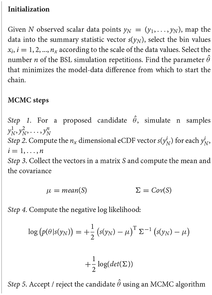
Algorithm 1. MCMC sampling of a Bayesian Synthetic likelihood with eCDF summary statistics.

ALGORITHM 2

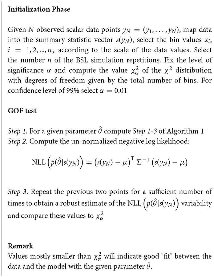
Algorithm 2. Goodness of fit test.

Note that as the likelihood is re-created at every sampling iteration, the log(det(Σ)) term needs to be included. When using eCDFs for summary statistics, one has to select the bin values at which the cumulative sums are evaluated. Too dense bin values produce noisy histograms and CDFs, resulting in close to singular covariance matrices and low acceptance rates in MCMC sampling in our situation. On the other hand, too few values tend to loose information of the data. Earlier experiences [13, 14, 24] have shown that the sampled parameter posteriors are not sensitive with respect to the specific selection of the number n_x of the bins, as long as the above extremes are avoided. Unless otherwise stated, all the examples of this paper are computed using n_x = 10.

Remark: For the sake of readability, Algorithm is formulated assuming only one eCDF vector is used as the summary statistics. More typically we employ several feature vectors. In such a case, the above steps are repeated separately for each feature vector and the resulting eCDF vectors are concatenated to get the final vector. The concatenated vector of Gaussian vectors is Gaussian again, and the mean and covariance of that vector provides the likelihood function. The normality of the combined feature vector is numerically verified in the same way as described earlier.

2.2. Assessing the goodness of the model fits

Above, we assume that a robust estimate of the region of the parameter space at which to start sampling efficiently is available. In case of synthetic data sets there exists, by construction, a region of the parameter space for which the model can quantitatively and qualitatively re-produce the statistics of the reference data. However, when fitting a model to real data a bias can be expected, and a test for goodness of fit (or lack of fit) is needed. Standard criteria, based on residual sums of the fit, are not available in the stochastic setting discussed here. We discuss here how to employ ingredients used to perform the Gaussianity tests employed in the initialization phase of Algorithm for a goodness of fit (GOF) test. Given a set of parameters, this will tell us how appropriate a model is in representing the underlying dynamics that produced the data.

Note that for any fixed set of parameters (as in this GOF tests) the likelihood's mean and covariance are fixed as well and the $\frac{1}{2}log\left[det(\Sigma )\right]$ term is not used for the negative log likelihood (NLL) calculation. The procedure is a version of the classical χ² tests used as a standard tool since [25], only the construction and evaluations of the likelihood function are done in a different way.

In a nutshell the goodness of fit test proceeds as follows:

This procedure can help in several crucial aspects. It can be helpful in understanding whether the model is or is not appropriate to represent the underlying dynamics that generated the data, and indicate possible needs for further model selection. Moreover, before starting the MCMC sampling, it can be used to see if the optimizer has already found an appropriate region of the parameter space. If this is not the case, it shows how far from the data the model is at the initial parameter value. The latter case may be due to a genuine lack of fit, or it may indicate that the optimizer has got stuck in a local minimum. In Section 4, examples of lack of fit are given when using a proxy for the volatility process. We demonstrate how this may result in biased estimates, and show how to avoid it (see Figure 8).

2.3. Kalman filter and kernel density estimation methods

We will compare our results with those obtained by the basic Kalman filter (KF) approach, see for instance [26]. In a more demanding situation, where KF runs into difficulties, we employ a more advanced ensemble approach as an alternative to produce kernel density estimates that approximate the SDE transition probabilities.

Given an infinite number of simulations for SDEs, one could theoretically construct SDE model transition densities to obtain the solution to Fokker-Planck equations. In practice, we are limited to a finite number of simulations which we can use to approximate the transition densities p(y_n+1∣y_n). We can use a kernel density estimator to approximate the transition densities in order to numerically evaluate the likelihood function ${\displaystyle \prod _{n=1}^{N-1}p(y_{n+1}\mid y_n)}$. An ensemble of simulations is computed for each pair of consecutive data points (y_n, y_n+1), starting at the data point y_n. Given more accurate model parameter estimates, the simulated trajectories should follow the data more closely. This results in higher likelihood values for more correct parameters values.

The simulations are then used to construct a transition density which is evaluated at the next data point y_n+1, yielding an estimate for the transition likelihood for the given parameters. Such an approach has been used for maximum likelihood estimation of SDE parameters [9]. We follow the authors in using a Gaussian kernel as the kernel. For more details on the density estimation procedure, see [9]. Instead of maximum likelihood estimation as used by [9], we use the kernel density estimates to compute the likelihood of the SDE model parameters. This enables the use of an MCMC method to estimate the posterior distribution of the SDE model parameters. The BSL and the kernel density estimation (KDE) share the similarity in their approach, that they both rely on ensembles of simulations to construct a likelihood estimate for the SDE parameters. The information provided by the simulations is used in different ways, which results in a considerable difference in the required number of simulations. We discuss this in more detail in Section 4.

2.4. Noisy Markov chain Monte Carlo sampling

As discussed above, we employ empirically Gaussian likelihoods for parameter sampling and standard MCMC sampling algorithms may be used. However, the likelihood values are stochastic by construction, and need to be re-evaluated at each MCMC step during the BSL likelihood sampling. Depending on the data and number of BSL simulations n, the acceptance rate may get low. In such a case, the acceptance rate can be dramatically improved by using higher values for n, in the range 1, 000 < n < 3, 000. Essentially the same parameter posteriors were obtained for high and low values of n by increasing the chain length of sampling for low n. But this comes at the cost of higher CPU demands. The possibility of low acceptance rate for low n values is due to uncertainty in the estimates of the mean and covariance of the BSL likelihood. Increased n values stabilize those estimates, thus leading to higher acceptance rates. A remedy is to use noisy MCMC sampling [27, 28]. A high rejection rate of a stochastic likelihood function typically is due to the fact that the negative log likelihood can get exceedingly low values simply due to the stochasticity. The idea behind the noisy sampling is to re-evaluate the likelihood function at the same parameter value where the sampling has been stuck. In our examples, we perform the re-evaluation if 200 consecutive rejections have taken place. This allows us to achieve reliable posterior estimates with lower values of n.

3. Test cases

The approach introduced in Section 2 is applied here to several SDE models with increasing difficulty of parameter estimation. We start with the well–known Ornstein-Uhlenbeck model that allows for comparison to standard estimation methods. Next, the Merton model is discussed as a situation where these standard methods actually fail. Finally, we study a test case for the widely-used Heston stochastic volatility model.

3.1. Ornstein-Uhlenbeck model

The standard one-dimensional Ornstein-Uhlenbeck model for a mean reverting process is

$\begin{array}{ll}d{X}_t=-\theta X_{t}dt+\sigma d{W}_t,& (4)\end{array}$

where θ is the rate of mean reversion and σ the diffusion coefficient for the Wiener process W_t. As the reference values for the model parameters we will use (θ, σ) = [0.5, 1]. The Euler-Maruyama algorithm with a time step Δt is used for numerical integration to compute the values X_i, i = 1, 2, ..., N. For simplicity, we take data at every integration time step. This setting is used in order to allow for a direct comparison with estimates obtained via a standard filtering method. Filtering methods are based on prediction / correction steps, and so the observation time step cannot be much larger than the integration time step to enable the prediction. Figure 1 exhibits an example trajectory.

FIGURE 1

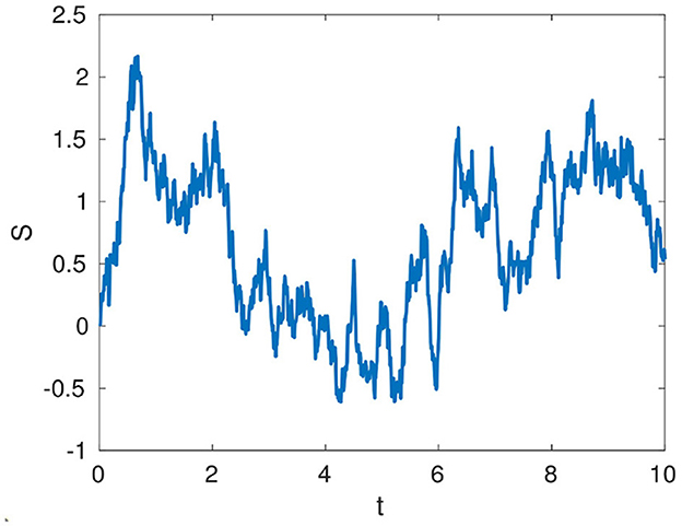
Figure 1. An example Ornstein-Uhlenbeck trajectory with (θ, σ) = [0.5, 1] in the time interval [0, 10], computed by the Euler-Maruyama integration with time step Δt = 0.01.

3.2. Merton model

A more complex example, when it comes to parameter estimation, is the Merton model [29]. It is the Ornstein-Uhlenbeck process where a “jump” component is added via a Poisson process. The model equation can be written as

$\begin{array}{ll}d{X}_t=-\theta X_{t}dt+\sigma d{W}_t+dq;& (5)\end{array}$

where (θ, σ) are the same parameters as in the Ornstein-Uhlenbeck system, and q(t) denotes an independent Poisson process for jumps, with the frequency of the jumps given by a Poisson parameter λ. Moreover, the size for each jump is randomly sampled from Z_t~N(μ, ϵ). Figure 2 exhibits an example trajectory.

FIGURE 2

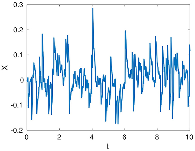
Figure 2. An example Merton trajectory with (θ, σ, λ) = [10; 0.08; 10], and (μ, ϵ) = [0.01, 0.1] in the time interval [0, 10], computed by the Euler-Maruyama integration with time step Δt = 0.01. The expected time of arrival times of the jumps is given by λΔt.

3.3. Heston model

Finally, we demonstrate the feasibility of our method by applying it to a task from the field of insurance risk management. The Heston stochastic volatility model has originally been introduced to price options under the risk-neutral measure [30]. Under the corresponding risk-neutral dynamics, any traded asset, such as, e.g., a non-dividend-paying stock must grow on average at the risk-free rate. While this risk-neutral measure is useful for the valuation of derivatives, it is also artificial, chosen in such a way that pricing corresponds to taking the risk-neutral expectation of the payoff and discounting at the risk-free rate. Risk management, in contrast, requires actual probabilities, e.g., of losing more than 5% of the value of a portfolio of stocks over a given time horizon. The physical measure gives the actual probability of occurrence of events and the Heston model under this measure is commonly used in risk management practice to predict future returns or volatility from historical time series, for instance in Solvency Capital Requirement calculations (see, e.g., [2]). Therefore, we concentrate here on the Heston model for modeling a stock price S under the physical measure, see Figure 3. As is common practice in parameter estimation, we have to stationarize the data which is done by using returns rather than prices. The corresponding system of Heston SDEs reads

$\begin{array}{llll}d{S}_t/S_t& =& (r+\eta v_t)dt+\sqrt{v_t}(\sqrt{1-{\rho }^2}d{W}_t^1+\rho d{W}_t^2),& (6)\end{array}$

$\begin{array}{llll}d{v}_t& =& k(\theta -v_t)dt+ϵ\sqrt{v_t}d{W}_t^2,& (7)\end{array}$

FIGURE 3

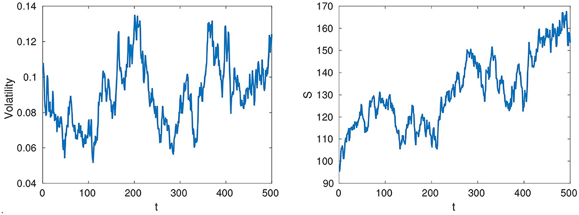
Figure 3. Example Heston trajectories with daily observations in the time interval [0, 500] with reference parameters [θ, k, ϵ, ρ, λ₁] = [0.1, 3, 0.25,−0.8, 4], computed by the QE-scheme. (Left) Instantaneous volatility. (Right) Stock price.

where S denotes the stock price process and v the unobservable instantaneous volatility process. W¹ and W² are independent Wiener processes. Furthermore we have the following model parameters:

• r risk-free rate of return

• θ long run average price variance

• k rate of mean reversion to θ_p

• ϵ volatility of volatility

• ρ correlation parameter between the Wiener processes.

We require the Cox-Ingersoll-Ross process of the volatility v to be strictly positive, therefore we impose the Feller condition 2kθ>ϵ². Under the physical measure, the expected return includes an additional premium in excess of the risk-free rate. This so-called equity premium η is the compensation for the diffusive risk and can be estimated from the stock price time series alone. Note that η could be further partitioned into the compensation for market risk per unit of dW₁ and volatility risk per unit of dW₂, i.e., $\eta ={\lambda }_1\sqrt{1-{\rho }^2}+{\lambda }_2\rho$. However, this partition can not be inferred without including another class of observations, namely option prices observed in the market and therefore we set λ₂ = 0. While both λ₁ and λ₂ could in principle be estimated by including option price time series, this comes at a massive computational cost (cf. [8]), and is therefore left for future research.

In practice, only the time series of the prices S can be observed directly so that in order to estimate the corresponding parameters of the Heston model, a proxy for the unobserved volatility process is required. A number of possible constructions for proxies have been suggested such as realized volatility measures [31, 32], integrated volatility proxies and Black-Scholes implied volatility proxies [6] and more recently, the VIX index published by the Chicago Board Options Exchange (CBOE), see [33], has been used as a proxy for the S&P 500 index volatility (see, e.g., [2, 7, 8, 34]). In our experiments we study the Heston system, first supposing that time series for both S and v have been observed directly—reproducing an experimental setup from [6, 7]. Next, we employ the same data but use only the time series for the stock price S, and create the observational data for the volatility by a proxy, namely, the Black-Scholes implied volatility of an at-the-money option with expiry in one month from the observation time. In both cases, parameter estimation relies on the assumption that the underlying system for the given data is the Heston model. Last, in order to correct for the bias introduced by using the proxy, we propose a model with Heston stock price dynamics and volatility evolving according to the proxy dynamics for use in the estimation algorithm.

It is well-known that the square root function in (6) increases the bias for the standard Euler-Maruyama and Milstein scheme (cf. [35]). In order to simulate both, stock price and volatility data, we therefore employ the QE scheme by Andersen (see [36]). We consider a test setup from [6, 7], to be precise, we use sample lengths of 500 transitions at daily sampling intervals Δ = 1/252. We generate a sample path using the QE scheme using thirty sub-intervals per sampling interval Δ where twenty nine out of every thirty observations are discarded which yields observations at the desired daily frequency. The simulation is initialized with the stock at 100 and the instantaneous volatility v₀ initialized at its long run mean. The parameter values for the generation of the data are [θ, k, ϵ, ρ, λ₁] = [0.1, 3, 0.25,−0.8, 4] and the risk-free rate is fixed at 3.0%. Figure 8C exhibits example trajectories for both the stock price and volatility process. Note, however, that we can not compare our results directly to the those obtained in [6, 9], as these maximum likelihood methods do not allow for uncertainty quantification out of the box, in fact the bias and standard deviation reported there correspond to repeated maximum likelihood computations with different data via a Monte Carlo method, while in the present work we use merely one fixed data set. However, the posterior distributions presented in the next section roughly agree with the variability of the individual parameter uncertainties reported in [6].

Remark: We would like to emphasize here, that our test setting assuming the comparably small number of merely 500 daily observations reflects the requirements of real-world applications. On the one hand, stock price time series with significantly more than 500 daily observations will most probably cover different market regimens so that fitting these with only one set of Heston parameters is in general not feasible. On the other hand, using intraday data to increase the number of observations is also not recommendable as the Heston model does not take into account market micro-structure effects (see, e.g., [37]).

4. Numerical results and discussion

In this section we use the three test models discussed in the previous Section to compare the numerical results obtained by our method to those given by the other methods presented in Section 2, as well as with earlier results presented in literature. Additionally, we assess the goodness of fit for the models to the given observational data.

4.1. Ornstein-Uhlenbeck

In order to use the BSL method with the eCDF summary statistics, two features are extracted from the computed time series: The solutions X_i, and the time differences ΔX_i = X_i+1−X_i. The latter is necessary identify the diffusion parameter σ reliably, see also [13]. Separate eCDFs are computed for both features, which then are combined to build the final feature vector. To further clarify the role of the selected features, Figure 4, shows the impact of employing each feature separately. Using only the feature vector constructed with the eCDF of the state values X_i, i = 1, 2, ..., N, produces a posterior distribution which is narrow with respect to the mean reverting parameter θ but wide (though limited) in the direction of σ. On the other hand, using only the time differences X_i+1−X_i, i = 1, 2, ..., N produces a posterior distribution that is more accurate with respect to σ but wide in the direction of the θ parameter. The intersection of the two posterior regions yields a “small“ set of sampled points. Indeed, using both features, concatenating the respective vectors into one vector, gives the posterior in Figure 4 that roughly coincides with the intersection set.

FIGURE 4

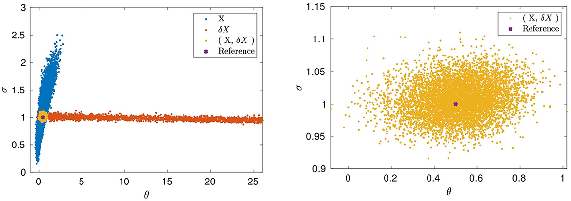
Figure 4. Ornstein-Uhlenbeck posteriors with data in the time interval [0, 10], time step Δt = 0.01, using BSL with n = 100 simulations. (Left) Only the state X used (blue), respectively, only the differences of consecutive points ΔX used (red). (Right) Ornstein-Uhlenbeck posterior when the combination of both (X, ΔX) is used (yellow).

As stated in Section 2 (and see [13]), the normality of the eCDF vectors holds also in non i.i.d. cases, assuming the data is weakly correlated. In our present situation the observations are taken dense in time and clearly are not i.i.d. But the normality can be verified by the χ² test and component-wise scalar normality tests.

In case of the Ornstein-Uhlenbeck model, we can compare the result obtained by with the BSL approach against the estimation results obtained by the well-known Kalman filter likelihood (KF). The comparison with Kalman filter is performed using the Example 11.5 from the textbook [26]. The KF data and posterior come from [26] and for the same fixed data set we perform both the KF and the BSL estimation for data values y_t in the interval t∈[0, 10] with integration time step 0.1, N = 100 data points and n = 100 BSL simulations. The sampled parameter posteriors naturally move depending on the simulated data created for the MCMC sampling experiment. The example in Figure 5 presents a typical case, showing how the BSL posteriors generally agree with the samples by KF. The result comes, however, at higher costs in terms of CPU times: BSL here uses n = 100 simulations for each likelihood evaluation, whereas the KF requires only one. Concerning the comparison to the KDE method we would like to emphasize that the computational complexity of that method exceeds that of the BSL method. We observed that significantly higher numbers of SDE realizations were required for the KDE approach. In order to achieve proper MCMC convergence, we used 1,000 SDE realizations to construct the likelihood estimates. This in clear contrast to the 100 realizations we use for one step of the MCMC sampling with BSL. The problem is further exacerbated in the Merton and Heston cases. For the Merton and Heston models, we use 200 realizations with the BSL MCMC sampling. The KDE approach required 15,000 realizations for proper MCMC sampling.

FIGURE 5

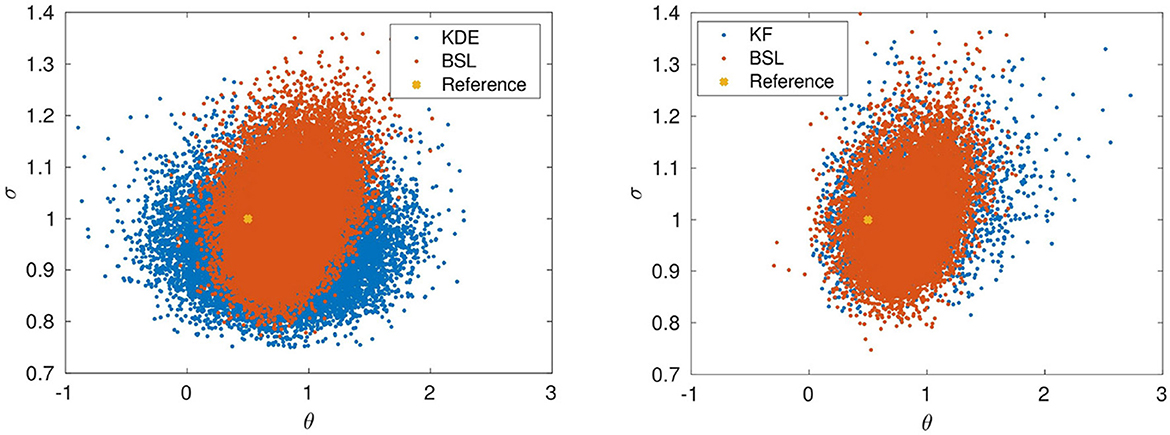
Figure 5. Ornstein-Uhlenbeck posterior for the reference parameters (θ, σ) = [0.5; 1] obtained by (Right) using KF (blue), respectively BSL (red). (Left) Using KDE (blue), respectively BSL (red). N = 100 data points on the interval [0, 10], with integration time step Δt = 0.1.

The two-dimensional posterior distribution obtained with the KDE approach is illustrated in Figure 2. For the kernel density results, we used an MCMC chain with 10⁶ samples. In this case the result shows clearly a wider range of possible values for the speed of mean reversion parameter θ.

To further verify the robustness of the approach with respect to the “tuning” parameters, the selection of the bin parameter n_x and the BSL simulations n, an extensive series of test runs was performed. Both values were varied in a wide range, 6 ≤ n_x ≤ 20 and 100 ≤ n ≤ 3000. For each selection, the MCMC sampling of the parameter posterior was repeated 20 times, each time using different data sets simulated by the Ornstein-Uhlenbeck model with the same settings as those used for producing Figure 5. In each case the outcome was compared with the result obtained by KF. The overall conclusion was that the parameter posteriors obtained by BSL and KF essentially coincide.

Note that the BSL estimation works equally well with arbitrarily sparse (but pairwise, to get the differences X_i+1−X_i) observations, while the KF and other filtering methods need sufficiently close data points to produce meaningful predictions, as they are all based on the prediction/correction steps. In the next example we discuss a case where this property—no prediction required—becomes more crucial.

4.2. Merton

Next, we use the BSL algorithm with eCDF statistics for a jump-diffusion system. Using the Euler-Maruyama integration for Equation (5), we simulate N = 1, 000 data points; for the parameter estimation we use n = 500 BSL simulations. In this case, it is natural that the estimation may fail if the frequency of the jumps is too low compared to the integration time interval—trivially so if no jumps happen to occur in the measurement data set. Also, if the jumps are too small and dense the Poisson jumps dq will be confounded with the Ornstein-Uhlenbeck diffusion process. Figure 2 presents the type of data we are aiming at: A set with sufficiently many jumps, most of them clearly distinguishable, thus enabling the parameter estimation. The number of BSL simulations n must now be increased compared to the previous test case and higher n values produce more stable estimates for the mean and covariance of the likelihood function. Lower n values technically work as well, but lead to more stochastic likelihood value evaluations, and thus lower acceptance rates in the MCMC sampling. Figure 6A shows the BSL parameter posteriors for all the five parameters to be estimated. The two feature vectors are constructed in the same way as in the previous test case, using the state values and the differences of consecutive state values. We can observe that all parameters are well identified, whereas the presence of jumps render the prediction difficult for filtering methods. One way to estimate posterior distributions for the Merton parameters with the kernel density approach is to use two simultaneous models, one without Poisson jumps occurring and a second with a Poisson jump occurring. We used the maximum likelihood estimate to select between these two processes whether a jump occurred at the current increment. The kernel density estimates for the processes were used to compute the maximum likelihood estimates. Note that, this approach does not directly provide an estimate for the Poisson rate parameter λ. However, λ can be estimated via bookkeeping: During the simulation of each MCMC sample, we can save the information whether a jump occurred and the differences between these locations can be used to estimate the Poisson parameter. For the Merton kernel density results, we used an MCMC chain with 5 × 10⁴ samples. Figure 6B shows that the KDE method constructed this way is yields somewhat unreliable results as the reference value for σ does not even lie inside the posterior and is therefore outperformed by the BSL method.

FIGURE 6

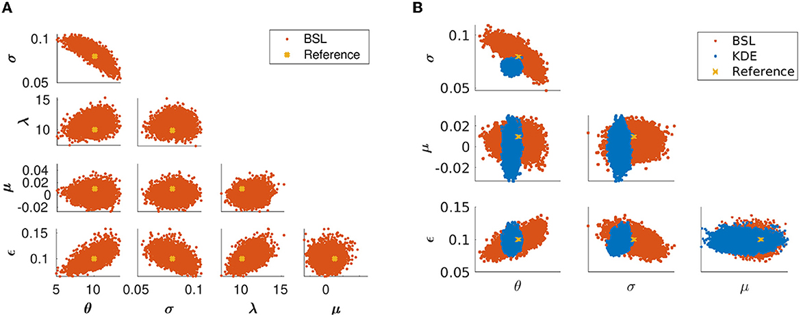
Figure 6. (A) Parameter posteriors of the Merton model for the reference parameters (θ, σ) = [10;0.08] and (λ, μ, ϵ) = [10, 0.01, 0.1], obtained using BSL with data size N = 1, 000 and n = 100 simulations. (B) Comparison with KDE. Parameter posteriors of the Merton model for KDE (blue) and BSL (red).

Remark: Note that in this work, we focus on explaining the novel BSL method and therefore keep the underlying financial models as simple as possible. Nevertheless, it should be emphasized that this method is model-agnostic and works equally well for more sophisticated models that include jumps such as the long memory Fractional Barndorff-Nielsen and Shephard model (cf. [38]).

4.3. Heston

As in the previous examples, we take the state components and their time differences as the scalar quantities whose empirical cumulative density functions give the feature vectors for the likelihood. As our approach requires boundedness of these quantities, we consider the returns (ΔS_t/S_t), with ΔS_t = S_t+1−S_t rather than the state values S_t. The volatility evolves according to the CIR Equation (7) and therefore remains bounded (which is also the case for the volatility proxy introduced below), so both volatilities and their time differences Δv: = v_t+1−v_t can be used to define features. Based on the structure of the model, it is beneficial to add additional feature vectors: As the Wiener processes W¹ and W² in Equations (6) and (7) are connected by the correlation parameter ρ, it is a natural choice to compute the correlation coefficient between the simulated stock price and volatility. The estimation accuracy can be further increased by adding more features extracted from the data, e.g., the mean and standard deviation of the volatility can be used to further stabilize the estimation. For this purpose, we divide the available data into d subsets y⁽¹⁾, …, y^(d) and compute the mean and standard deviation for each of the subsets. An additional feature vector is then constructed for the statistics of this subset data. For example, given N = 500 observed data points, we can cut the data to obtain d = 25 subsets of 20 successive data points each, and compute the corresponding means and standard deviations. For these 25 means and standard deviations, we can again compute the mean and standard deviation of both to arrive at a 4−dimensional vector. The final feature vector is a concatenation of all the feature vectors created.

To sum up, given the stock price S_t and the volatility v_t, the feature vector used for estimating the parameter values of the Heston model is the concatenation of the following:

• empirical CDF of ΔS/S

• empirical CDF of v

• empirical CDF of Δv

• correlation coefficient of ΔS/S with Δv

• the mean and the standard deviation of the mean and standard deviation of the volatility.

For every newly sampled parameter, a set of n samples, each consisting of N points, is simulated. The likelihood is computed at every step by estimating the mean and the covariance matrix of the feature vector as described in Section 2 and evaluated against the given data.

First, we assume that the latent volatility process is observable and we apply both the BSL method with n = 200 simulations and a KDE method using an MCMC chain with 5 × 10³ samples to the observational data. The results are illustrated in Figure 7. Most of the reference values lie within the posteriors for both methods with slightly smaller estimation uncertainty for the BSL method. However, the parameter ρ lies just on the tail of the KDE posterior.

FIGURE 7

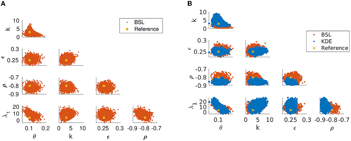
Figure 7. Parameter posteriors of the Heston model with observed volatility for the reference parameters [θ, k, ϵ, ρ, λ₁] = [0.1, 3, 0.25,−0.8, 4], obtained using BSL with data size N = 500 daily observations and n = 200 simulations. (A) Posterior distribution obtained with BSL (red). (B) Comparison of the posterior distributions obtained respectively by using the BSL (red) and KDE (blue) methods.

Next, we consider the more realistic setting where we can only observe a proxy volatility, namely the Black-Scholes implied volatility of an at-the-money option with expiry in 1 month from the observation time. Note that the example data used for the following computation differs from the data used for the previous example and as mentioned earlier, the sampled parameter posteriors naturally move depending on the simulated data created for the MCMC sampling experiment. Figure 8C illustrates the fact that the proxy volatility systematically underestimates the true Heston volatility process. Figure 8B shows the same issue but in a quantitative way via the goodness of fit test, see Algorithm 2. It suggests that we should not fit the Heston model to stock price data simulated according to (6) and volatility data given by the Black-Scholes implied volatility proxy. Figure 8B illustrates what happens if we do so nevertheless: The goodness of fit test for the maximum of the posterior (MAP) indicates a good fit, however, this fit is severely biased regarding the parameters κ and ϵ. Thus, if we are interested in these parameters in the standard Heston model (6), (7), we should replace the true volatility (7) in the BSL simulation with the Black-Scholes implied volatility proxy, thus correcting for the unavoidable observation bias.

FIGURE 8

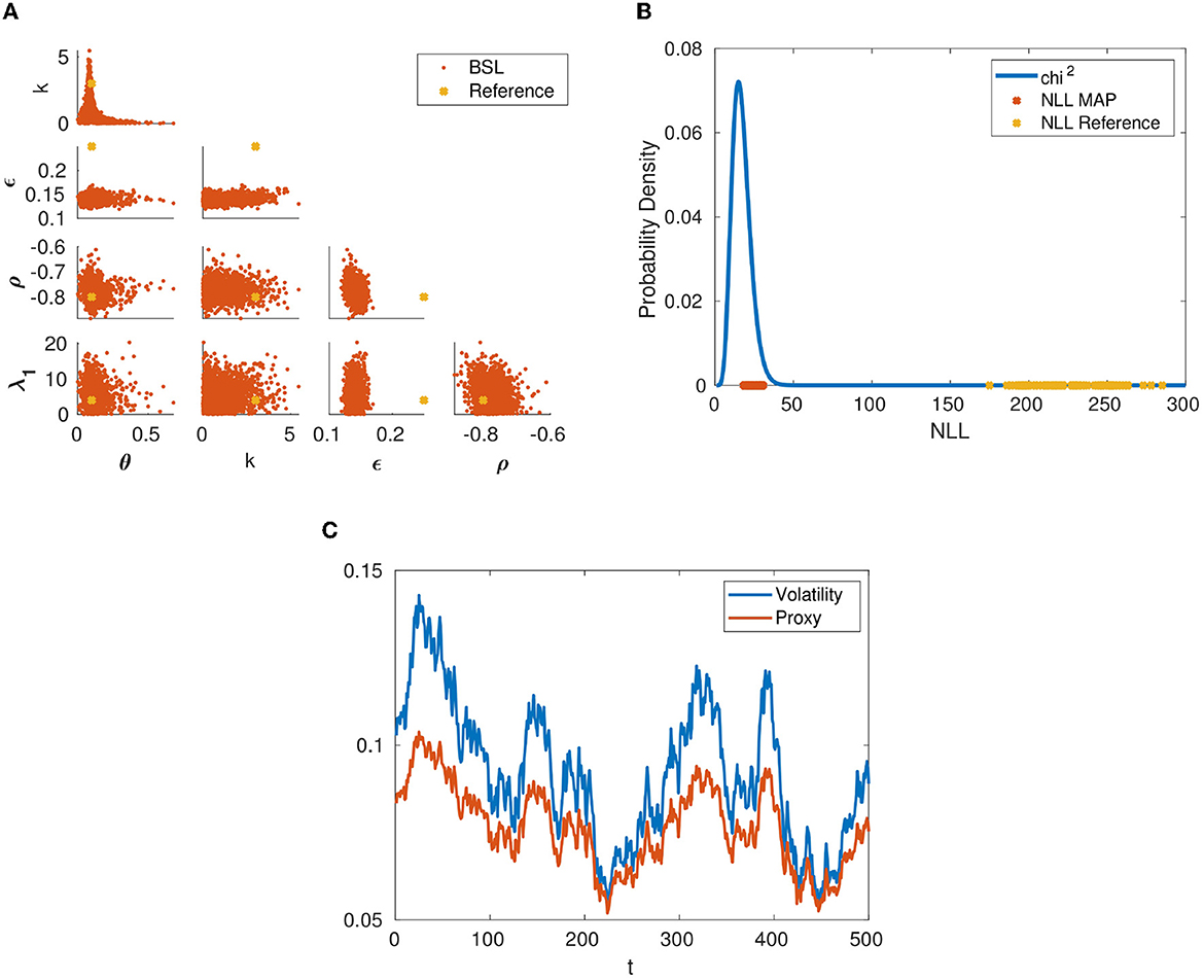
Figure 8. (A) Parameter posterior of the Heston model with observed proxy volatility for the reference parameters [θ, k_p, ϵ, ρ, λ₁] = [0.1, 3, 0.25,−0.8, 4], obtained using BSL with data size N = 500 daily observations and n = 200 simulations. (B) Goodness of fit obtained with the Heston model for the reference parameters [θ, k_p, ϵ, ρ, λ₁] = [0.1, 3, 0.25,−0.8, 4] (yellow) and parameters given by the posterior distribution MAP (red). (C) Comparison between the instantaneous volatility and the volatility proxy for a trajectory obtained with the same parameter values.

As expected, based on the goodness of fit test, the model provides a reasonably good fit to the observed data. The posterior distribution and the goodness of fit test for the estimation using this “corrected” Heston model are illustrated in Figures 9A, B, respectively. Summarizing, we have seen via the goodness of fit test for the MAP estimate, that the observed stock price data and volatility proxy data given by the Black-Scholes implied volatility of an at-the-money option could in principle be fit by the standard Heston model. However, both the posterior distribution and another goodness of fit test for the reference parameter values reveal that the corresponding parameter estimates will be heavily biased. Our BSL estimation using the “corrected” Heston model with the volatility proxy instead of the true volatility (7) does not suffer from this bias. This underlines the importance of testing against synthetic test data in order to validate estimation models, particularly given the fact that it seems to be a usual practice to use the standard Heston model in practical parameter estimation where only proxy data is available.

FIGURE 9

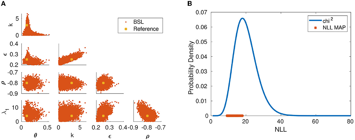
Figure 9. (A) Parameter posterior of the “corrected” Heston model with observed proxy volatility for the reference parameters [θ, k_p, ϵ, ρ, λ₁] = [0.1, 3, 0.25,−0.8, 4], obtained using BSL with data size N = 500 daily observations and n = 200 simulations. (B) Goodness of fit obtained with the “corrected” Heston model for parameters given by the posterior distribution MAP.

We note that [6] also shows results for 5, 000 observations. This case was repeated using the BSL method as well, again with similar estimation accuracies as those reported in [6]. We skip these results here, also since a comparison to the KDE approach turned out to be out of reach, due to the computational complexity of KDE.

5. Conclusions

In this work we have introduced the BSL method for the task of estimating parameters in systems of SDEs from time series data. In principle, a correct way of producing the parameter estimates is via integrating the Fokker-Plank equation and approximate solutions of this equation can be obtained by kernel density estimation methods. However, the parameter posteriors created that way can be unreliable, e.g., for jump diffusion models, and the required ensemble size easily leads to exceedingly high CPU demands. Our approach is based on a characterization of the variability of the data points by cumulative distribution functions. The stochastic feature vector created in this way is Gaussian which allows for the use of standard statistical methods such as MCMC sampling. This estimator has been shown to perform well even for small observational data sets. In cases of theoretically known parameter posteriors such as in the Ornstein-Uhlenbeck model, our results coincide with the analytical ones. For the practically relevant Heston stochastic volatility model, we have provided novel insights on how to construct a robust estimator including uncertainty quantification given proxy volatility data. These findings yield a promising avenue for future research using the BSL approach coupled with the empirical distribution as statistics. We mention the VIX index calculated by the Chicago Board Options Exchange (CBOE) as a volatility proxy. Moreover, the BLS method is model-agnostic so that, e.g., studying the parameter estimation problem for rough volatility models could also be an interesting topic for future research.

Data availability statement

The raw data supporting the conclusions of this article will be made available by the authors, without undue reservation.

Author contributions

HH and MS designed the study with input from all authors. MS has been responsible for the financial aspects presented. RM and SS wrote the code for the BSL approach and the GOF test and carried out the respective simulations while TH took care of the KDE simulations. RM prepared the figures. All authors discussed the results and shared the responsibility of writing the manuscript. All authors contributed to the article and approved the submitted version.

Funding

This work was supported by the Centre of Excellence of Inverse Modeling and Imaging (CoE), Academy of Finland, decision number 312 122. MS would like to acknowledge support by the German Federal Ministry of Education and Research (BMBF) under Grant No. 03FHP191. The content is solely the responsibility of the authors.

Conflict of interest

The authors declare that the research was conducted in the absence of any commercial or financial relationships that could be construed as a potential conflict of interest.

Publisher's note

All claims expressed in this article are solely those of the authors and do not necessarily represent those of their affiliated organizations, or those of the publisher, the editors and the reviewers. Any product that may be evaluated in this article, or claim that may be made by its manufacturer, is not guaranteed or endorsed by the publisher.

References

1. Berkowitz JP, DeLisle RJ. Volatility as an asset class: holding VIX in a portfolio. J Altern Invest. (2018) 21:52–64. doi: 10.3905/jai.2018.21.2.052

CrossRef Full Text | Google Scholar

2. Van Dijk MT, De Graaf CS, Oosterlee CW. Between ℙ and ℚ: the ℙℚ measure for pricing in asset liability management. J Risk Financ Manage. (2018) 11:67. doi: 10.3390/jrfm11040067

PubMed Abstract | CrossRef Full Text | Google Scholar

3. Lautier D, Javaheri A, Galli A. Filtering in finance. Wilmot Mag. (2003) 5:67–83. doi: 10.1002/wilm.42820030315

CrossRef Full Text | Google Scholar

4. Wang X, He X, Zhao Y, Zuo Z. Parameter estimations of Heston model based on consistent extended Kalman filter. IFAC-PapersOnLine. (2017) 50:14100–5. doi: 10.1016/j.ifacol.2017.08.1850

CrossRef Full Text | Google Scholar

5. Ruiz E. Quasi-maximum likelihood estimation of stochastic volatility models. J Econ. (1994) 63:298–306. doi: 10.1016/0304-4076(93)01569-8

CrossRef Full Text | Google Scholar

6. Aït-Sahalia Y, Kimmel R. Maximum likelihood estimation of stochastic volatility models. J Financ Econ. (2007) 83:413–52. doi: 10.1016/j.jfineco.2005.10.006

PubMed Abstract | CrossRef Full Text | Google Scholar

7. Hurn AS, Lindsay KA, McClelland A. A quasi-maximum likelihood method for estimating the parameters of multivariate diffusions. J Econ. (2013) 172:106–26. doi: 10.1016/j.jeconom.2012.09.002

CrossRef Full Text | Google Scholar

8. Hurn AS, Lindsay KA, McClelland AJ. Estimating the parameters of stochastic volatility models using option price data. J Bus Econ Stat. (2015) 33:579–94. doi: 10.1080/07350015.2014.981634

CrossRef Full Text | Google Scholar

9. Hurn AS, Lindsay KA, Martin VL. On the efficacy of simulated maximum likelihood for estimating the parameters of stochastic differential Equations. J Time Ser Anal. (2003) 24:45–63. doi: 10.1111/1467-9892.00292

PubMed Abstract | CrossRef Full Text | Google Scholar

10. Pedersen AR. A new approach to maximum likelihood estimation for stochastic differential equations based on discrete observations. Scand J Stat. (1995) 22:55–71.

PubMed Abstract | Google Scholar

11. Aït-Sahalia Y. Closed-form likelihood expansions for multivariate diffusions. Ann Stat. (2008) 36:906–37. doi: 10.1214/009053607000000622

CrossRef Full Text | Google Scholar

12. Särkkä S. Bayesian Filtering and Smoothing. Cambridge University Press (2013).

Google Scholar

13. Maraia R, Springer S, Haario H, Hakkarainen J, Saksman E. Parameter estimation of stochastic chaotic systems. Int J Uncertain Quant. (2021) 11:49–62. doi: 10.1615/Int.J.UncertaintyQuantification.2020032807

CrossRef Full Text | Google Scholar

14. Haario H, Kalachev L, Hakkarainen J. Generalized correlation integral vectors: a distance concept for chaotic dynamical systems. Chaos. (2015) 25:063102. doi: 10.1063/1.4921939

PubMed Abstract | CrossRef Full Text | Google Scholar

15. Wood SN. Statistical inference for noisy nonlinear ecological dynamic systems. Nature. (2010) 466:1102–4. doi: 10.1038/nature09319

PubMed Abstract | CrossRef Full Text | Google Scholar

16. Price LF, Drovandi CC, Lee A, Nott DJ. Bayesian synthetic likelihood. J Comput Graph Stat. (2018) 27:1–11. doi: 10.1080/10618600.2017.1302882

CrossRef Full Text | Google Scholar

17. Neumeyer N. A central limit theorem for two-sample U-processes. Stat Probabil Lett. (2004) 67:73–85. doi: 10.1016/j.spl.2002.12.001

CrossRef Full Text | Google Scholar

18. Donsker MD. Justification and extension of Doob's heuristic approach to the Kolmogorov-Smirnov theorems. Ann Math Stat. (1952) 23:277–81. doi: 10.1214/aoms/1177729445

CrossRef Full Text | Google Scholar

19. Dickhaus T. Some extensions. In: Theory of Nonparametric Tests. Springer (2018). p. 119–26. doi: 10.1007/978-3-319-76315-6_8

CrossRef Full Text | Google Scholar

20. Borovkova S, Burton R, Dehling H. Limit theorems for functionals of mixing processes with applications to U-statistics and dimension estimation. Trans Am Math Soc. (2001) 353:4261–318. doi: 10.1090/S0002-9947-01-02819-7

CrossRef Full Text | Google Scholar

21. Fasiolo M, Wood SN, Hartig F, Bravington MV. An extended empirical saddlepoint approximation for intractable likelihoods. Electron J Stat. (2018) 12:1544–78. doi: 10.1214/18-EJS1433

CrossRef Full Text | Google Scholar

22. An Z, Nott DJ, Drovandi C. Robust Bayesian synthetic likelihood via a semi-parametric approach. Stat Comput. (2020) 30:543–57. doi: 10.1007/s11222-019-09904-x

CrossRef Full Text | Google Scholar

23. Thomas O, Dutta R, Corander J, Kaski S, Gutmann MU. Likelihood-free inference by ratio estimation. Bayesian Anal. (2022) 17:1–31. doi: 10.1214/20-BA1238

CrossRef Full Text | Google Scholar

24. Springer S, Haario H, Susiluoto J, Bibov A, Davis A, Marzouk Y. Efficient Bayesian inference for large chaotic dynamical systems. Geosci Model Dev. (2021) 14:4319–33. doi: 10.5194/gmd-14-4319-2021

PubMed Abstract | CrossRef Full Text | Google Scholar

25. Pearson K. On the criterion that a given system of deviations from the probable in the case of a correlated system of variables is such that it can be reasonably supposed to have arisen from random sampling. London Edinburgh Dublin Philos Mag J Sci. (1900) 50:157–75. doi: 10.1080/14786440009463897

CrossRef Full Text | Google Scholar

26. Särkkä S, Solin A. Applied Stochastic Differential Equations. Institute of Mathematical Statistics Textbooks. Cambridge University Press (2019).

Google Scholar

27. Nicholls G, Fox C, Watt A. Coupled MCMC with a randomized acceptance probability (2012).

Google Scholar

28. Medina-Aguayo F, Lee A, Roberts G. Stability of noisy metropolis-hastings. Statist Comput. (2016) 26:1187–211. doi: 10.1007/s11222-015-9604-3

PubMed Abstract | CrossRef Full Text | Google Scholar

29. Merton RC. Option pricing when underlying stock returns are discontinuous. J Financ Econ. (1976) 3:125–44. doi: 10.1016/0304-405X(76)90022-2

CrossRef Full Text | Google Scholar

30. Heston SL. A closed-form solution for options with stochastic volatility with applications to bonds and currency options. Rev Financ Stud. (1993) 6:327–43. doi: 10.1093/rfs/6.2.327

CrossRef Full Text | Google Scholar

31. Barndorff Nielsen OE, Shephard N. Non-Gaussian Ornstein-Uhlenbeck-based models and some of their uses in financial economics. J R Stat Soc Ser B. (2001) 63:167–241. doi: 10.1111/1467-9868.00282

CrossRef Full Text | Google Scholar

32. Andersen TG, Bollerslev T, Diebold FX, Labys P. The distribution of realized exchange rate volatility. J Am Stat Assoc. (2001) 96:42–55. doi: 10.1198/016214501750332965

PubMed Abstract | CrossRef Full Text | Google Scholar

33. CBOE. The CBOE Volatility Index–VIX: The Powerful and Flexible Trading and Risk Managment Tool From the Chicago Board Options Exchange. CBOE (2014).

Google Scholar

34. Pfante O, Bertschinger N. Uncertainty of volatility estimates from Heston greeks. Front Appl Math Stat. (2018) 3:27. doi: 10.3389/fams.2017.00027

CrossRef Full Text | Google Scholar

35. Lord R, Koekkoek R, Van Dijk A D. A comparison of biased simulation schemes for stochastic volatility models. Quant Finan. (2010) 10:177–94. doi: 10.1080/14697680802392496

CrossRef Full Text | Google Scholar

36. Andersen L. Simple and efficient simulation of the Heston stochastic volatility model. J Comput Finan. (2008) 11:1–43. doi: 10.21314/JCF.2008.189

CrossRef Full Text | Google Scholar

37. El Euch O, Fukasawa M, Rosenbaum M. The microstructural foundations of leverage effect and rough volatility. Finan Stochast. (2018) 22:241–80. doi: 10.1007/s00780-018-0360-z

CrossRef Full Text | Google Scholar

38. Salmon N, SenGupta I. Fractional Barndorff-Nielsen and Shephard model: applications in variance and volatility swaps, and hedging. Ann Finan. (2021) 17:529–58. doi: 10.1007/s10436-021-00394-4

CrossRef Full Text | Google Scholar