 Bernardo Cockburn
 Shukai Du2
- 1School of Mathematics, University of Minnesota, Minneapolis, MN, United States
- 2Department of Mathematics, University of Wisconsin-Madison, Madison, WI, United States
- 3Facultad de Matemáticas y Escuela de Ingeniería, Instituto de Ingeniería Matemática y Computacional, Pontificia Universidad Católica de Chile, Santiago, Chile
We provide a short introduction to the devising of a special type of methods for numerically approximating the solution of Hamiltonian partial differential equations. These methods use Galerkin space-discretizations which result in a system of ODEs displaying a discrete version of the Hamiltonian structure of the original system. The resulting system of ODEs is then discretized by a symplectic time-marching method. This combination results in high-order accurate, fully discrete methods which can preserve the invariants of the Hamiltonian defining the ODE system. We restrict our attention to linear Hamiltonian systems, as the main results can be obtained easily and directly, and are applicable to many Hamiltonian systems of practical interest including acoustics, elastodynamics, and electromagnetism. After a brief description of the Hamiltonian systems of our interest, we provide a brief introduction to symplectic time-marching methods for linear systems of ODEs which does not require any background on the subject. We describe then the case in which finite-difference space-discretizations are used and focus on the popular Yee scheme (1966) for electromagnetism. Finally, we consider the case of finite-element space discretizations. The emphasis is placed on the conservation properties of the fully discrete schemes. We end by describing ongoing work.
1. Introduction
We present a short introduction to the devising of a particular type of numerical methods for linear Hamiltonian systems. The distinctive feature of these methods is that they are obtained by combining finite element methods for the space-discretization with symplectic methods for the time-discretization. The finite element space discretization of the Hamiltonian system is devised in such a way that it results in a system of ODEs which is also Hamiltonian. This guarantees that, when the system is discretized by a symplectic method, the resulting fully discrete method can conserve the linear and quadratic time-invariants of the original system of ODEs. This is a highly-sought property, especially for long-time simulations.
For a description of the pioneering work and of the development of these methods, the reader can see the Introductions in our papers published in 2017 [1], in 2021 [2], and in 2022 [3] and the references therein. In those papers, other approaches to achieve energy-conserving schemes are also briefly reviewed. Particularly impressive are the schemes proposed in 2019 by Fu and Shu [4] in which the authors construct energy-conserving discontinuous Galerkin (DG) methods for general linear, symmetric hyperbolic systems.
When we began to study this type of numerical methods for linear Hamiltonian systems, we were impressed to see that the methods displayed arbitrary high-order accuracy and preserved (in time) very well the energy and other quantities of physical relevance. Although we were familiar with finite element space discretizations, we were unaware of the relevance and properties of the symplectic time-marching methods. In a way, the paper we present here is the paper we would have liked to read as we plunged into this topic. It is written as an introduction to the subject for numerical analysts of PDEs which, like us, were not familiar with symplectic methods.
We restrict ourselves to the linear case for two reasons. The first is that we have studied those numerical methods for Hamiltonian formulations of acoustic wave propagation, elastodynamics and the Maxwell's equations. So, we do have some experience to share for those systems. The second is that the theory of symplectic time-marching can be covered quite easily and that most of its results also hold in the nonlinear case, although they are not that easy to obtain.
Let us sketch a rough table of contents:
• Hamiltonian and Poisson Systems. (Section 2) We define a general Hamiltonian (and its simple extension, the Poisson) systems, of ODEs or PDEs. We then restrict ourselves to linear systems, give several examples, and discuss the conservation laws associated to them. For the Hamiltonian and Poisson systems, we took material from the books that appeared in 1993 by Olver [5], in 1999 by Marsden and Ratiu [6], in 2004 by Leimkuhler and Reich [7], and in 2010 by Feng and Qin [8]. For the conservation laws, we took the information gathered in our papers on the acoustic wave equation in 2017 [1] elastodynamics in 2021 [2], and electromagnetism in 2022 [3, 9].
• Symplectic and Poisson time-marching methods. (Section 3) We describe the symplectic (and their simple, but useful, extensions to the Poisson) methods for linear Hamiltonian ODEs with special emphasis on how they approximate their linear and quadratic invariants. We took material from the pioneering work of the late 1980's by Feng et al. [10–12], from the popular 1992 review by Sans-Serna [13], from the 2006 book by Hairer et al. [14], and form the 2010 book by Feng and Qin [8].
• Finite Difference space discretizations. (Section 4) We show how to discretize in space the linear Hamiltonian systems by using finite difference methods. In particular, we recast as one of such schemes the popular Yee scheme for electromagnetism proposed in 1966 [15], that is, more than 17 years before the appearance of the first symplectic method. We took material from the work done in 1988 by Ge and Feng [10] and in 1993 by McLachlan [16].
• Finite Element space discretizations. (Section 5) We describe space discretizations based on finite element methods and combine them with symplectic time-marching schemes. We discuss the corresponding conservation properties and show a numerical experiment validating a couple of them. We took material from the work done in 2005 by Groß et al. [17], in 2008 by Xu et al. [18], and by Kirby and Kieu [19], as well as from our own work in 2017 [1], 2021 [2], and 2022 [3, 9].
• Ongoing work. (Section 6) We end by briefly commenting on some ongoing work.
2. Hamiltonian and Poisson systems
2.1. Canonical Hamiltonian systems and their generalization
2.1.1. The canonical nonlinear Hamiltonian systems
A canonical Hamiltonian system is defined on (the phase-space) ℝ2n in terms of the smooth Hamiltonian functional and a structure matrix J by the system of equations
where1
The Hamiltonian has the remarkable property of remaining constant on the orbits of the system, t ↦ u(t). Indeed,
since the matrix J is anti-symmetric. This computation suggests an immediate extension of this Property to other functionals. If is any differentiable functional, we have that
and we can see that remains constant on the orbits of the system, t ↦ u(t), if and only if the Poisson bracket, , is zero. Such quantities are usually called first integrals of the system. They are also called invariants or conserved quantities.2
2.1.2. A generalization
This definition can be generalized by taking a phase space of arbitrary dimension, by allowing J to be an arbitrary anti-symmetric matrix, or by letting it depend on the phase-space variable u, that is, by using J: = J(u). In these cases, the system is called a Poisson system.
A Poisson dynamical system is, see the 1993 books [5, 16], the triplet , where is the phase-space, is the Hamiltonian functional, and {·,·} is the Poisson bracket. The system can then be expressed as
The Poisson bracket {·,·} is a general operator with which we can describe the time-evolution of any given smooth function . This operation is defined for a pair of real-smooth functions on the phase-space satisfying: (i) bilinearity, (ii) anti-symmetry, (iii) Jacobi identity:
and, (iv) the Leibniz' rule:
for . For a constant anti-symmetric matrix J, usually called the structure matrix, these four properties are trivially satisfied by the induced Poisson bracket, see the 1993 book by Olver [5, Corollary 7.5].
2.2. Definition of linear Hamiltonian and Poisson systems
As we restrict ourselves to linear Hamiltonian and Poisson systems, let us formally define them. All the definitions are in terms of the structure matrix J (which is anti-symmetric), but, to alleviate the notation, we omit its mention.
Definition 2.1 (Hamiltonian systems). We say that the linear system
is Hamiltonian if the structure matrix J (which is anti-symmetric) is invertible and the Hamiltonian is a quadratic form for some symmetric matrix H.
Definition 2.2 (Poisson systems). We say that the linear system
is a Poisson system if J is a structure matrix (which is anti-symmetric) and the Hamiltonian is a quadratic form for some symmetric matrix H.
We see that a Poisson system is the straightforward generalization of a Hamiltonian system,3 to the case in which the structure matrix is not invertible.4
2.3. Examples of linear Hamiltonian systems of ODEs
Let us illustrate and discuss examples of linear Hamiltonian systems and their respective symplectic structure.
Example 1. A textbook example of a linear canonical Hamiltonian system is the system modeling the harmonic oscillator. Its Hamiltonian and structure matrix are
This gives rise to the Hamiltonian system of equations
We know that the restriction of the Hamiltonian to the orbits of this system is constant in time, or, in other words, that the quadratic form is a first integral of the system. This implies that the orbits lie on circles. No interesting property can be drawn from a linear first integral of the system since the only one it has is the trivial one.
Example 2. The following is a simple example in which the structure matrix J is not invertible. We work in a three-dimensional space (we take u: = (p, q, r)⊤) and consider the system associated with the following Hamiltonian and structure matrix:
This gives rise to the Poisson system
Let us examine the conserved quantities of the system. Again, we know that the restriction of the Hamiltonian to the orbits of this system is constant in time, or, in other words, that the quadratic form is a first integral of the system. This implies that the orbits lie on spheres. Unlike the previous case, this system has one linear first integral,5 namely, C(p, q, r): = (0, 1, 1)·(p, q, r), as this reflects the fact that q+r is a constant on the orbits of the system. This has an interesting geometric consequence since it means that the orbits of the system lie on the intersection of a sphere and a plane of normal (0, 1, 1), see Figure 1.
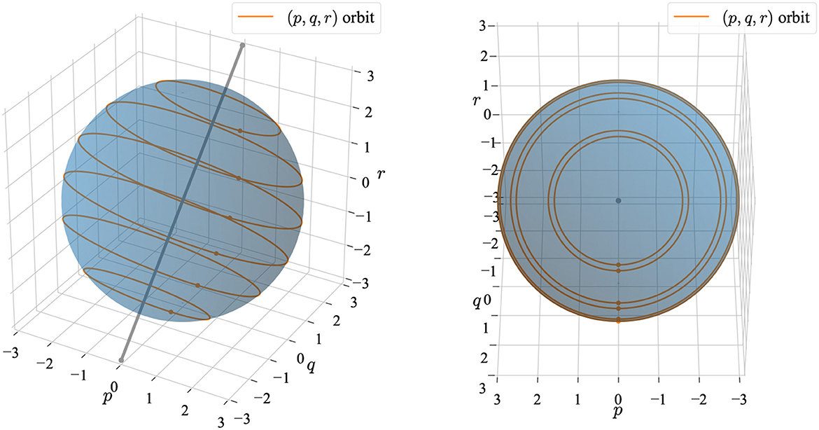
Figure 1. Two views of the orbits (orange solid line) of the Poisson system on the phase-space (q, p, r). The orbits are circles (right) lying on planes (left) with normal (0, 1, 1) so that q + r is a constant. The blue sphere represents the constant Hamiltonian value corresponding to .
2.4. Hamiltonian PDEs: Definition and examples
To extend the definition of finite-dimensional Hamiltonian and Poisson systems, the triplet , to systems of partial differential equations, we need to introduce a phase-space of smooth functions with suitable boundary conditions (periodic for simplicity), a Hamiltonian functional , and a Poisson bracket {·,·}. The definition of the bracket is induced by an anti-symmetric structure operator J, for functionals on the phase-space defined by
It satisfies bilinearity, anti-symmetry, and the Jacobi identity (Leibniz's rule is dropped). In the definition the operation δ/δu denotes the functional derivative defined for functionals on by
for any smooth test function δv in . Thus, a Hamiltonian partial differential equation system is given by
An important simplification occurs in the case when the structure operator J is a constant, anti-symmetric operator whose definition might include spatial differential operators. In this case, the Jacobi identity is automatically satisfied. See Olver [5, Corollary 7.5].
Let us define and illustrate the Hamiltonian6 systems of PDEs we are going to be working with.
Definition 2.3 (Linear Hamiltonian PDE system). We say that the linear system of partial differential equations
is a Hamiltonian system for any constant structure operator J (which is anti-symmetric), inducing the Poisson bracket {·,·}, and the Hamiltonian functional is a quadratic form (meaning that is linear in v).
2.4.1. The scalar wave equation
Let us consider the linear scalar wave equation on a bounded, connected domain Ω ⊂ ℝd with smooth boundary ∂Ω
Where ρ is a scalar-valued function and κ a symmetric, positive definite matrix-valued function. Here the unknown u can be a variety of physical quantities. For example, in acoustics, it represents the deviation from a constant pressure of the medium. In water waves, it represents the distance to the position of rest of the surface of a liquid. Here, we take advantage of its closeness to the vector equations of elastodynamics,7 and we formally assume that u has the dimensions of a length. We can then introduce the velocity variable v, and rewrite the equation as a first-order system of equations as follows:
This system can be written in a Hamiltonian form with Hamiltonian functional, and the canonical structure operator J defined by
Indeed, observe that the variational derivatives of the Hamiltonian functional are
for δu, δv smooth test functions with compact support on Ω.
A second and equivalent Hamiltonian form can be found as follows. We rewrite the scalar wave equations as a first-order system introducing the vector-valued function q = κ▽u and removing u from the equations, this is known as the mixed formulation
This system can also be written in a Hamiltonian form with an equivalent Hamiltonian functional, now in terms of v and q, and the structure operator J defined by
The Poisson bracket is then induced by the operator, for functionals F, G
Thus,
where f = ▽·(κF).
In Tables 1, 2, we describe the conservation laws associated with the linear scalar wave equation. See Example 4.36 in Olver [5], and in Walter [32].
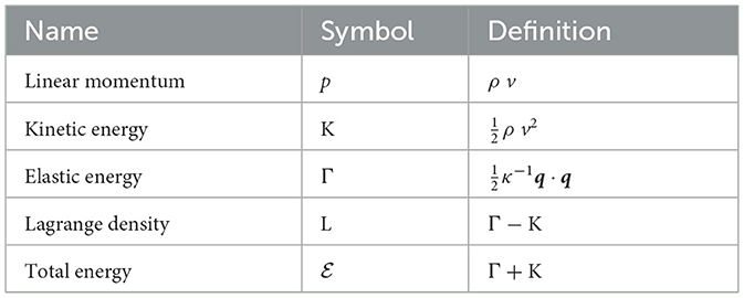
Table 1. Glossary of scalar wave equation quantities.
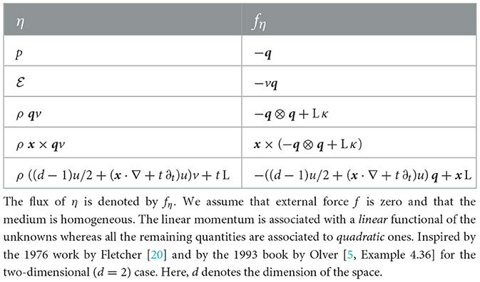
Table 2. Conservation laws for the scalar quantity η, , deduced from the scalar wave equation.
2.4.2. Electromagnetics
Our last example is the Maxwell's equations for the electric and magnetic fields,
The Hamiltonian form of these equations corresponds to the Hamiltonian functional and anti-symmetric operator given by
Where J× satisfies ▽ × J× = J. A second Hamiltonian formulation can be derived by introducing the magnetic vector potential variables A, by μH = ▽ × A, and writing the system as follows
with corresponding Hamiltonian functional and anti-symmetric operator given by
In Tables 3, 4, we describe the rich set of conservation laws associated to the Maxwell's equations. The first two are associated with the conservation of charge, magnetic and electric. The next three are the classic conservation laws of energy and momenta. Less standard are the last three, which were obtained back in 1964 by Lipkin [21]. See the 2001 paper [33] for a recent update on the classification of conservation laws of Maxwell's equations.
Table 3. Glossary of electromagnetic quantities, see Sánchez et al. [3].
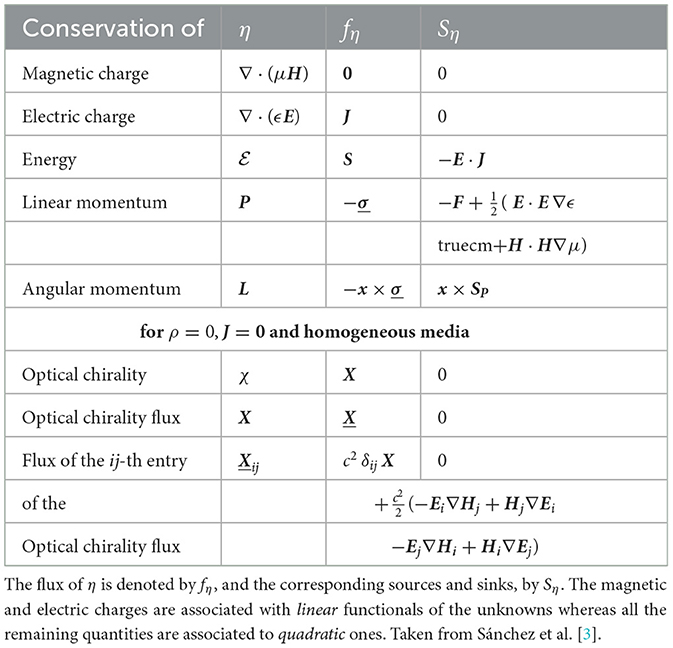
Table 4. Conservation laws for the (scalar or vectorial) electromagnetic quantity η, , deduced from the first two Maxwell's equations.
3. Symplectic and Poisson time-marching methods
As pointed out in the 1992 review by Sanz-Serna [13], the symplectic time-marching methods were devised specifically for the time-discretization of Hamiltonian systems. In this section, we present a simple and direct introduction to the topic, with emphasis on Poisson linear systems, which seems to be new. The approach we take reflects our own path into the subject and is intended for readers that, like us, were utterly and completely oblivious to the relevance of symplectic and Poisson matrices, and were only interested in devising numerical methods for Hamiltonian systems which would capture well their conservation properties. The main objective of this section is to overcome this terrible, terrible shortcoming.
3.1. Symplectic and Poisson matrices
Here, we introduce the symplectic (and their simple extension, the Poisson) matrices which are, as we are soon going to see, deeply related to Hamiltonian (and their simple extension, the Poisson) systems. We use the definitions from the 2006 book by Hairer et al. [14, p. 254].
Definition 3.1 (Symplectic matrices). We say that the invertible matrix E is a symplectic matrix for the structure matrix J (which is anti-symmetric) if J is invertible and if E⊤J−1E = J−1.
Definition 3.2 (Poisson matrices). We say that the invertible matrix E is a Poisson matrix for the structure matrix J (which is anti-symmetric) if it satisfies EJE⊤ = J. If, in addition, E⊤ = Id on the kernel of J, we say that E is a Poisson integrator matrix.
Note that, since
the definition of a Poisson matrix is a straightforward generalization of the definition of a symplectic matrix to the case in which the structure matrix is not necessarily invertible. Note also that the difference between Poisson matrices and Poisson integrator matrices is that the behavior of the transpose of the latter on the kernel of the structure matrix is explicitly specified.
3.1.1. The geometry of Poisson matrices
We next gather what we could call the geometric properties of the Poisson matrices. To state it, we introduce some notation. The kernel of a matrix M is denoted by M−1{0}. Its range is denoted by Mℝd. Although we do not assume the structure matrix J to be invertible, we can always define its inverse on part of the space ℝd. Indeed, since the restriction of J to Jℝd is a one-to-one mapping, we can define J−1 as the inverse of J on Jℝd.
Proposition 3.1 (The geometry of Poisson matrices). Let E be a Poisson matrix. Then
Moreover, if E is also a Poisson integrator matrix, then
for some matrix B: ℝd→Jℝd.
This result states that a Poisson matrix E is one-to-one on the range of J and behaves as a symplectic matrix8 therein, see property (b). Moreover, its transpose is also one-to-one on the kernel of J. If the matrix is also a Poisson integrator, that is, its transpose is the identity on the kernel of J, then E coincides with the identity plus a matrix whose range is included by the range of J.
Proof of Proposition 3.1 Let us prove (a). Since E is a Poisson matrix, we have that EJ = JE−⊤, and so EJℝd⊂Jℝd. We also have that E−1J = JE⊤, and so E−1Jℝd⊂Jℝd. This proves Property (a).
Let us prove (b). Since the restriction of J to Jℝd is a one-to-one mapping, we can define J−1 as the inverse of J on Jℝd. Then, since E is a Poisson matrix, on Jℝd, we have that J = E−1JE−⊤ and so, that J−1 = E⊤J−1E, because EJℝd = Jℝd by Property (a). This proves Property (b).
Let us now prove (c). Since E is a Poisson matrix, we have that JE⊤ = E−1J, and so E⊤J−1{0}⊂J−1{0}. We also have that E−⊤J−1{0}⊂J−1{0}. This proves Property (c).
It remains to prove (d). Since E is a Poisson integrator, the kernel of E⊤−Id includes the kernel of J. As a consequence, the range of E−Id is included in the range of J. This proves Property (d).
The proof is now complete. ⃞
3.1.2. The evolution operator
Our first result states that Hamiltonian (Poisson) systems and symplectic (Poisson) matrix integrators are deeply related in an essential manner.9
Proposition 3.2 (The evolution matrix is a Poisson integrator matrix which commutes with A). Consider the Poisson system , where A = JH. Then,
Proof. Let us prove that E(t) is a Poisson matrix. We have that
because J⊤ = −J. As a consequence, we get that E(t)JE⊤(t) = E(0)JE⊤(0) = J. This proves that E(t)JE⊤(t) = J for all t∈ℝ.
Let us now complete the proof of Property (i) by showing that E⊤(t)v = v for all v in the kernel of J. Observe that
Thus, E⊤(t)v = E⊤(0)v = v.
Property (ii) clearly holds. This completes the proof. ⃞
3.1.3. Conserved quantities
Next, we characterize all possible linear and quadratic functionals which remain constant on the orbits of any linear system. It does not have to be a Hamiltonian system.
Proposition 3.3 (Characterization of linear and quadratic first integrals). Let t↦u(t) be any of the orbits of the linear system . Then,
(i) The mapping ↦ vTu(t) is constant if and only if ATv = 0,
(ii) If the matrix S is symmetric, the mapping t ↦ uT(t)S u(t) is constant if and only if S A + ATS = 0.
For Poisson systems, a couple of simple consequences can be readily obtained. The first is that, in (i), the linear functional t↦v⊤u(t) is constant in time if and only if A⊤v = −HJv = 0. In other words, the system has linear first integrals if only and only if either J or H is not invertible. If they are, then so is A⊤ and the only linear first integral of the system is the trivial one.
The second consequence is that, in (ii), we can take S: = H. Indeed, SA+A⊤S = HJH+HJ⊤H = 0, because J is anti-symmetric. This shows that, for any Hamiltonian system, the Hamiltonian is always a quadratic first integral.
Proof. Let us prove Property (i). We have
This implies Property(i).
Let us now prove Property (ii). We have
and we see that, for the last quantity to be equal to zero, the matrix A⊤S+SA has to be anti-symmetric. Since this matrix is also symmetric, because S is symmetric, it must be identically zero. This implies Property (ii) and completes the proof. ⃞
3.2. Approximate Poisson evolution operators commuting with A
From now on, we focus on finding out when it is possible to guarantee that the linear and quadratic first integrals of the original Hamiltonian system are also maintained constant after discretization. We give a characterization of the Poisson Runge-Kutta methods and show that these methods do conserve the linear and quadratic first integrals of the original Hamiltonian. This exact conservation property is the first main result of this section. It justifies the relevance of Poisson numerical methods for the time-discretizations of Hamiltonian ODEs.
So, consider now the approximation un to u(Δtn) given by the one-step numerical scheme
If EΔt is a symplectic matrix, we say that the scheme is symplectic. If EΔt is a Poisson matrix, we say that the scheme is a Poisson scheme.
Clearly, the discrete evolution matrix EΔt is an approximation to the exact evolution matrix E(Δt) = eAΔt. Since, by Proposition 0.0.2, the exact evolution matrix is a Poisson integrator matrix, one wonders what do we gain by requiring that the discrete evolution matrix EΔt to be also a Poisson integrator matrix.
It is possible to answer that question in a very satisfactory manner if we additionally require that the discrete evolution matrix EΔt commute with A. As we see next, if this is the case, the original Hamiltonian remains constant on the discrete orbits of the numerical scheme.
Proposition 3.4. Assume that
Then the mapping is constant.
Proof. Since
Where , we only have to show that Θ = 0.
We know that Jℝd⊕J−1{0} = ℝd so we can write un = Jw+v, for some w∈ℝd and v∈J−1{0}. Then, we insert this expression into the definition of Θ to obtain
where
by Property (d) of Proposition 3.1. We can rewrite these quantities in a more convenient manner with the help of the following matrix:
Indeed, we can now write that
But
Since EΔt is a Poisson matrix and commutes with A, we have that Φ = 0 on the range of EΔtJ, and, by Property (a) of Proposition 3.1, on the range of J. As a consequence, we get that Θ = v⊤Φv.
It remains to prove that v⊤Φv equals to zero. Since Jℝd⊕J−1{0} = ℝd, we can write that Hv = y+h where y is in the range of J and h in kernel of J. Since we can consider that J−1 is defined on the range of J, we can write that y = J−1x for some element x of the range of J. Then
because of the orthogonality of the kernel of J with its range. This completes the proof. ⃞
3.2.1. Evolution matrices which are rational functions of hA
Next, we consider an important example of evolution matrix EΔt satisfying the assumptions of the previous result, that is, EΔt is a Poisson integrator matrix and commutes with A.
Proposition 3.5. Set A: = JH where J is antisymmetric and H is symmetric. Set also EΔt: = R(ΔtA), where z↦R(z) is a rational function. Then, EΔt is a Poisson integrator matrix if and only if R(z)R(−z) = 1 and R(0) = 1.
This result has a simple and remarkable geometric interpretation. It states that the Poisson numerical methods whose evolution matrix is a rational function of hA are those for which we can recover the point we were evolving from by just applying the same scheme with time reversed, that is, the schemes for which,
Let us now prove the result.
Proof. Set Z: = ΔtA. By definition, the discrete evolution operator EΔt: = R(ΔtA) is a Poisson integrator matrix if
(i) R(Z)JR(Z)⊤ = J,
(ii) R(Z)⊤ = Id on the kernel of J.
We want to show that these two properties are equivalent to
(1) R(z)R(−z) = 1,
(2) R(0) = 1.
Since R is a rational function, there are polynomials P and Q such that R(z) = (Q(z))−1P(z). In terms of these polynomials, the above conditions read
(a) P(z)P(−z) = Q(z)Q(−z),
(b) P(0) = Q(0).
We only prove that (a) and (b) imply (i) and (ii), as the converse is equally easy.
Let v be an arbitrary element of the kernel of J. So (ΔtHJ)ℓv = 0, for ℓ>0, and since P is a polynomial matrix we have
By (b), we get
and then Property (ii) follows.
Let us prove Property (i). Take u: = Jw, where w is an arbitrary element of ℝd. By (a),
and since
because J is anti-symmetric, we get that
As this holds for all elements w of ℝd, we obtain that
and Property (i) follows. This completes the proof. ⃞
3.2.2. Symplectic Runge-Kutta methods
Perhaps the main example of numerical methods whose discrete evolution operator EΔt is a rational function of ΔtA is the Runge-Kutta methods. In fact, if the Butcher array of the Runge-Kutta method is

then
Where 11 is the s-dimensional column vector whose components are one, and, see [31],
This means that the previous result characterizes all the symplectic Runge-Kutta methods. Two important conclusions can be immediately drawn:
(i) No explicit Runge-Kutta method (that is, Q is not a constant) is symplectic.
(ii) Any Runge-Kutta method for which Q(z) = P(−z) is symplectic. Two notable examples are:
(α) The s-stage Gauss-Legendre Runge-Kutta method, which is of order 2s. The function R(z) is the s-th diagonal Padé approximation to ez.
(β) Any diagonally implicit Runge-Kutta method for which
The function R(z) is given by .
3.2.3. Conserved quantities
The Poisson integrator Runge-Kutta methods also maintain constant all the linear and quadratic first integrals of the original Poisson system. As pointed out above, this result unveils the importance of these methods for reaching our objective, namely, the conservation of the first integrals of the original Poisson system.
Theorem 3.1 (Exact conservation of linear and quadratic first integrals). All linear and quadratic first integrals of the original Poisson system remain constant on the orbits n↦un provided by a Poisson integrator Runge-Kutta method. That is,
Proof. Let us prove Property (i). We have
because the evolution matrix for Δt = 0 must be the identity, that is, R(0) = Id. This proves Property (i). Note we did not use that the numerical scheme is Poisson, we only used the form of the evolution operator.
Now, let us prove Property (ii). We have
Since SA = −A⊤S, we have that SP(ΔtA) = P(−ΔtA⊤)S, and, as a consequence, that
We can then write that
since the scheme is a Poisson integrator. This proves Property (ii) and completes the proof. ⃞
3.3. Poisson integrator matrices which do not commute with A
Now, we turn our attention to discrete Poisson methods whose evolution matrix EΔt does not commute with the matrix A defining the original system. The loss of this commutativity property has dire consequences, as the exact conservation of the original Hamiltonian cannot be guaranteed anymore. Indeed, as we saw in the proof of Proposition 3.4, when the structure matrix J is invertible and EΔt is symplectic, we have that
Which means that the original Hamiltonian is not maintained constant, as claimed.
Nevertheless, because the matrix evolution EΔt is a Poisson integrator matrix, we can still get
(i) the existence of a matrix AΔt such that AJ is symmetric and that ,
(ii) the non-drifting property of quadratic first integrals (on bounded orbits) of the original Hamiltonian.
The property (i) states that the discrete dynamics of the numerical scheme is exactly that of a dynamical system (Hamiltonian if EΔt is symplectic) defined by a matrix AΔt which we expect to converge to A as the discretization parameter Δt tends to zero. This property will allow us to obtain the non-drifting property (ii).
The non-drifting property (ii) states that, provided that the orbits are bounded, the original quadratic first integrals oscillate around the correct value for all times and are away from it a number proportional to the size of the truncation error of the numerical scheme. This remarkable, non-drifting property is the second main result of this section. This is why we are interested in working with Poisson integrators of this type.
3.3.1. The approximate Poisson system
We begin by showing that there is a Poisson system whose continuous orbits contain the discrete orbits generated by the evolution matrix EΔt.
Proposition 3.6. Let the mapping Δt → EΔt, where the discrete evolution matrix EΔt is a Poisson matrix, be continuous on (0, T) and such that EΔt = 0 = Id. Then, for Δt small enough,
(i) The matrix is such that AΔtJ is symmetric.
(ii) The orbits n↦un generated by the discrete evolution operator EΔt lie on the orbits t↦u(t) of the Poisson system .
Proof. Let us prove Property (i). We have to show that AΔtJ is symmetric. But, for Δt small enough, we can write
Using the fact that EΔt is Poisson, we get that
and so, we can write that
This proves Property (i).
It remains to prove Property (ii). But the discrete orbits are made of the points
Which lie on the orbit . This proves Property (ii) and completes the proof. ⃞
3.3.2. Closeness of the approximate system
Although Proposition 3.3, with A replaced by AΔt, gives information about the linear and quadratic first integrals of the new system , we are more interested in knowing how close are those invariants to those of the original system. We have then to relate the matrices A and AΔt in order to estimate how well the numerical scheme approximates the original quadratic first integrals.
We show that those matrices are as close as the order of accuracy of the numerical scheme. We say that the order of accuracy of the numerical scheme un+1 = EΔtun is p if
for some constant C independent of Δt.
Proposition 3.7. Assume that Δt ≤ ln(3/2)/max{||A||, ||AΔt||}. Then
Proof. We have that
because This implies that
Since ||etB−Id|| ≤ et||B||−1, we get that
because . This completes the proof. ⃞
3.3.3. Non-drifting of quadratic first integrals
We end by noting that the quadratic first integrals of the original Hamiltonian system do not drift on the discrete orbits generated by the numerical scheme.
Theorem 3.2 (Non-drifting property of the quadratic first integrals). Let the discrete evolution matrix EΔt be a Poisson matrix, and let n↦un denote any of its orbits. Assume that . Then
Proof. Since we have that
This completes the proof. ⃞
In the case in which S = H = J−1A, we can take to get that
and, if the scheme is of order p, we immediately get that
for Δt small enough. Since is constant, we see that does not drift in time, as claimed. Of course, for this to take place, λmin has to be strictly positive, which happens when is never equal to zero on the unit sphere v⊤v = 1.
3.4. Separable Hamiltonians and partitioned Runge-Kutta methods
Since there are no explicit symplectic Runge-Kutta methods for general Hamiltonians, one wonders if the situation changes for some subclass of Hamiltonians. It turns out that this is the case for the so-called separable Hamiltonians. Indeed, there are explicit, partitioned Runge-Kutta which are symplectic when applied to separable Hamiltonian systems. This is the third main result of this short introduction.
3.4.1. Separable Hamiltonians
If the Hamiltonian is separable, that is, if
and if the corresponding Hamiltonian system is of the form
it is interesting to explore schemes which treat the q- and p-components of the unknown u in different ways.
3.4.2. Partitioned Runge-Kutta methods
The so-called partitioned Runge-Kutta methods are of the form
and can be thought as associated to two Butcher arrays,

To emphasize its relation with the standard RK methods, we can rewrite them as
where and . We can see that we recover the standard RK methods whenever and .
3.4.3. Conservation of the original linear first integrals
It is clear that these methods have an evolution matrix which does not commute with A. Because of this, all the results in the previous subsection apply to them when they are symplectic. In addition, they maintain constant all the linear first integrals of the original Hamiltonian, not because of their symplecticity but because of the structure of their evolution matrix.
Theorem 3.3 (Exact conservation of linear first integrals). Suppose that the original Hamiltonian is separable. Then, all linear first integrals of the original Hamiltonian are also first integrals of any partitioned Runge-Kutta method.
Proof. We have that whenever A⊤v = 0. This completes the proof. ⃞
3.4.4. Symplecticity
We end this section by providing a characterization of the partitioned Runge-Kutta methods which are Poisson (or symplectic), see a detailed proof in Appendix A, and by showing that they can be explicit.
Proposition 3.8. Suppose that the original Hamiltonian is separable. A partitioned Runge-Kutta method is Poisson (or symplectic) if an only if
When the partitioned Runge-Kutta methods becomes a standard Runge-Kutta method, this result is equivalent to Proposition 3.5, as it can be seen after performing a simple computation.
3.4.5. Explicit methods
An important example symplectic partitioned Runge-Kutta methods have theA-matrices of the Butcher arrays of the following form:
These methods are charaterized by the two vectors b and , with the obvious notation, and can be efficiently implemented as follows:
There are two, low accuracy methods which, nevertheless, deserve to be mentioned as they are considered as classic. The first is the so-called the Symplectic Euler method. It is associated with the vectors b = 1, , and is first-order accurate. It reads:
The second is the Störmer-Verlet method. It is associated to the vectors b = [0, 1]⊤ and and is second-order accurate. It can be obtained by applying the Symplectic Euler method twice by using the Strang splitting, that is,
We can also write the method as follows:
Where and . This is precisely the time-marching scheme used in the well known Yee's scheme [15] for Maxwell's equations.
We end this section by noting that explicit partitioned Runge-Kutta methods of any (even) order of accuracy can be obtained, as was shown in 1990 by Yoshida [23].
3.5. Illustration
We end this section by illustrating the application of the implicit midpoint method (the lowest order, symplectic Runge-Kutta method) and the symplectic Euler method (the lowest order, symplectic partitioned Runge-Kutta method). We consider Example 2, introduced in Section 2.3. Both methods preserve the linear first integral exactly (see Theorem 3.1 for the implicit midpoint method and Theorem 3.3 for the symplectic Euler method), this is observed in Figure 2 where the approximate orbits lie on planes perpendicular to the kernel of J, the vector (0, 1, 1). The implicit midpoint preserves the Hamiltonian exactly (see Theorem 3.1) and the symplectic Euler computes a non-drifting approximation of it (see Theorem 3.2).
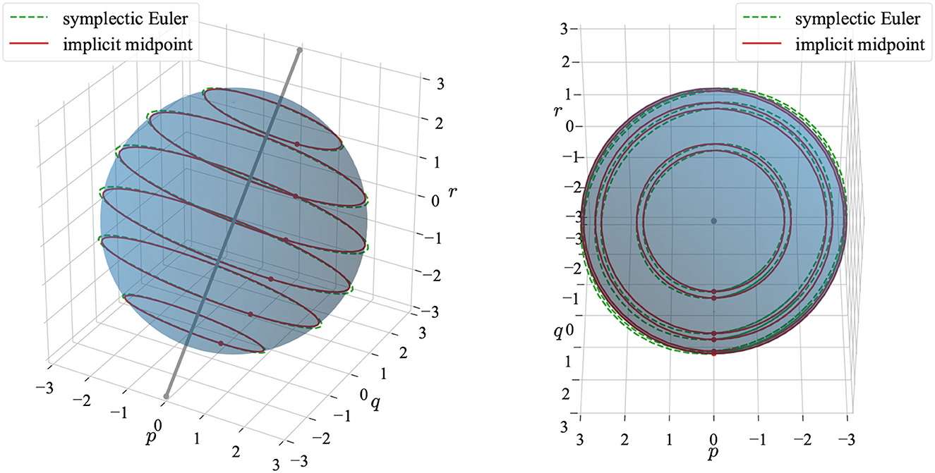
Figure 2. Two views of the approximate orbits of the Poisson system in Example 2 on the phase-space (p, q, r). The approximate orbits lie on planes with normal vector (0, 1, 1) so that q + r is a constant. The orbits in the dashed-green line were computed using the symplectic Euler method are ellipses and the ones in solid-red were computed using the implicit midpoint method and are circles. The blue sphere represents the constant Hamiltonian value corresponding to .
4. Symplectic finite difference methods
The idea of combining symplectic time integrators with finite difference spatial discretizations can be traced back to the late 1980's with the work of Feng and his collaborators [10, 11]. For instance, in 1987, Feng and Qi [11] applied symplectic integrators to the discretization in space by central difference schemes of the linear wave equation. In 1988, Ge and Feng [10] combined symplectic time-marching methods with finite difference schemes for a linear hyperbolic system. In 1993, McLachlan [16] incorporated the Poisson structure from Olver [5] to the design of symplectic finite difference schemes, and applied it to the non-linear waves, the Schrödinger, and the KdV equations. This effort continues. See, for example, the study of multisymplectic finite difference methods [24].
On the other hand, numerical methods (which are essentially symplectic time-marching methods applied to finite difference space discretizations) had been proposed much earlier (than 1980's) when the concept of symplectic time-integrators did not exist or was not systematically studied. A prominent example is Yee's scheme proposed in 1966 [15]. This scheme is also known as the finite-difference time-domain (FDTD) method, for which the acronym was first introduced in Taflove [25]. Later on, Yee's scheme was studied in the multisymplectic framework [26, 27]. However, to the best of our knowledge, no work exists which attempts recasting Yee's scheme as a combination of symplectic time-marching methods with finite difference space discretizations.
In this section, instead of attempting to reach for maximal generality, we focus on the Yee's scheme [15]. We show that the spatial discretization of the scheme leads to a Hamiltonian ODE system, while the time-discretization of the scheme is nothing but the well known, symplectic, second-order accurate Störmer-Verlet method. As a result, all the conservation properties of Section 3 hold for Yee's scheme.
4.1. The time-dependent Maxwell equations
Let us begin by recalling the time-dependent Maxwell's equations in the domain Ω = [0, L1] × [0, L2] × [0, L3]:
With periodic boundary conditions, where E and H represent the electric and the magnetic fields, respectively. If we set u = (E, H)T, we can rewrite the above equations into a more compact form:
where
Note Equation (6) is a Hamiltonian dynamical system with the triplet , where is the phase space, is the Hamiltonian
and the Poisson bracket is defined by
4.2. The space discretization of Yee's scheme
We next consider the spatial discretization of Yee's scheme [15], for which the electric and the magnetic fields are defined on the following grid points:
Namely, the magnetic field is defined on the edges and the electric field is defined on the faces of the cube element [iΔx, (i+1)Δx] × [jΔy, (j+1)Δy] × [kΔz, (k+1)Δz]. Let us denote by
the approximation spaces for the electric field E and the magnetic field H, respectively, and let z∈VE×VH be the vector representing the discretized electric and magnetic fields. Then, the spatial discretization of Yee's scheme introduces the following Hamiltonian system of ODEs:
where
In the above equations,
are the discretizations of the multiplication operation by ϵ and μ, respectively. Moreover,
are two different finite difference discretizations of the ∇ × operator. These operators will be described in full detail in the last subsection. Here we want to emphasize the abstract structure of the scheme as well as the main properties of these operators which are contained in the following result. A detailed proof is presented in Section 4.5.
Proposition 4.1. The operators and are symmetric and semi-positive definite. In addition, we have
Consequently, the operator J defined in Equation (7b) is anti-symmetric, and the operator H defined in Equation (7c) is semi-positive definite.
As a consequence of the above proposition, the ODE system (Equation 7a) is a Poisson dynamical system. In addition, thanks to the structure of J and H (see Equations 7b, 7c), we know its Hamiltonian is separable.
4.3. The fully discrete Yee's scheme
So we can now time-march this system of ODEs by using a symplectic scheme so that all the results of Section 3.4 hold.
In particular, if in the Equation (5), we replace q by E, P by H, Aqp by and Apq by , we obtain
and we recover Yee's scheme [15].
4.4. Conservation laws
Finally, we identify some conservation quantities associated to Yee's scheme. By Proposition 3.3, this task reduces to identify
• The kernel of A⊤. Suppose A⊤v = 0, then v⊤u is conserved in time.
• Symmetric matrix S such that SA+A⊤S = 0. Then, the bilinear form u⊤Su is conserved in time.
Before, we can present the main result, let us introduce some notation. For a given function fi, j, k, we define a shifting operator as follows:
In the above formulation, we allow the indexes i, j, and k to be non-integers so that the operator τ(s1, s2, s3) can be applied to fi, j, k on non-integer grid points. With this notation, we define the discretized Hamiltonian energy function
We also introduce two gradient operators
Where Th is the differencing operator given by
Note that the two gradients are defined on different grid spaces. The gradient ∇h, 0 is defined for function living on integer-grid points (i, j, k), while the gradient is defined on half-grid points . In addition, we remark that the range of ∇h, 0 is VH, and the range of is VE.
Proposition 4.2 (Conservation of energy and electric/magnetic charges). For the Yee's semi-discrete scheme defined by Equation (7a), the energy is conserved in time. In addition, (the weak form of) the electric and magnetic charges
is conserved in time. Here, ϕi (i = 1, 2) are arbitrary test functions.
4.5. Proof of proposition 4.1 and 4.2
In this subsection, we first define the operators , , , and . Then we prove Propositions 4.2 and 4.3.
We introduce two types of central difference operators and , which are defined as
Similarly, we can define , , , and . It is easy to observe that
Note that we have added the additional sub-indexes Hi to indicate the domain of the operators.
Lemma 4.1 (The anti-symmetry of central differences). We have
Proof. We will only prove that . The rest is similar. Notice that
This proves the claim. ⃞
Now, we define two discrete curl operators:
and
We also introduce the multiplication operators such that
The operator can be similarly defined.
Proof of Proposition 4.1 As we have seen, and are semi-positive definite since ϵ and μ are non-negative. Hence, the matrix H is semi-positive definite by its definition (Equation 7c). Moreover, by Lemma 4.1, we have that , and so, J is anti-symmetric. This completes the proof. ⃞
We are next going to prove Proposition 4.2. Before that, we will need a lemma.
Lemma 4.2 (The kernel of the finite difference curlh operators). We have that
Where Th is the differencing operator given by
Proof. We prove the lemma by a direct computation. Note that
Hence, Lemma 4.2-(i) holds. Lemma 4.2-(ii) can be proven in a similar manner. This completes the proof. ⃞
Proof of Proposition 4.2 Note that we have
Hence, to prove that is preserved in time, by Proposition 3.3, we only need to show that HA+A⊤H = 0, which is true since HA+A⊤H = HJH+H⊤J⊤H, J⊤ = −J, and H⊤ = H. Thus, the Hamiltonian is preserved in time on the discrete orbits of the numerical method.
Next, let us prove the conservation of the electric and magnetic charges. By Proposition 3.3, this task reduces to identify the kernel of A⊤. Since
by Lemma 4.2, we have
This completes the proof. ⃞
5. Symplectic-Hamiltonian finite element methods
This section presents the recent development of the so-called symplectic-Hamiltonian finite element methods for linear Hamiltonian partial differential equations. First, we discuss our results on energy-preserving hybridizable discontinuous Galerkin (HDG) methods for the scalar wave equation [1, 28], and then describe our further contributions to finite element discretizations of the linear elastic equation [2] and the Maxwell equations [3, 9]. We analyze in detail four finite element discretizations of the linear scalar wave (Equation 2) based on standard Galerkin methods, mixed methods, and HDG methods, and prove their structure-preserving properties.
5.1. Notation
Let us first introduce some standard finite element notation. For a given bounded domain Ω⊂ℝd, let be a family of regular triangulations of , with mesh-size parameter h the maximum diameter over the elements. We also assume for simplicity the elements are only simplices. For a domain D∈ℝd we denote by (·, ·)D the L2 inner product for scalar, vector and tensor valued functions
for (w, v)∈L2(D), (w, v)∈L2(D)d, and (w, v)∈L2(D)d×d. We extend these definitions for the inner product in (d−1)-dimensional domains. For discontinuous Galerkin methods, we define by the set of all element boundaries ∂K, for , and by the set of all the faces F of the triangulation . Inner product definitions are extended to these sets by
for properly defined scalar-valued functions w, v. Similar definitions are given for vector- and tensor-valued functions.
5.2. The continuous Galerkin method
We now present a standard finite element discretization of the linear scalar wave equation using H1-conforming approximations for the displacement and velocity variables. Let Vh be a continuous piece-wise polynomial subspace of , then the semi-discrete Galerkin method, corresponding to the primal formulation of the wave (Equation 3), reads as follows: Find (uh, vh)∈Vh×Vh such that
The system is initialized by projections of the initial conditions u0 and v0 onto the finite-dimensional space Vh. It is clear that the semi-discrete method inherits the Hamiltonian structure of the continuous (Equation 3) with triplet , where the discrete phase-space is , and the Hamiltonian and Poisson brackets are the respective restrictions to this space, i.e.
for linear functionals F = F[uh, vh], G = G[uh, vh], for uh, vh∈Vh, and where denotes the canonical anti-symmetric structure matrix .
Equivalently, we can formulate the method in its matrix form based on a given ρ-orthonormal basis {ϕi} of the space Vh and define the matrix and vector
Then, the evolution variables are represented in this basis by means of the coefficients u,v, i.e., and . We can write the Hamiltonian functional as a function of the coefficients y = (u,v)⊤ as
Therefore, computing the gradient of the Hamiltonian respect to the coefficients y = (u,v)⊤, we conclude that the standard Galerkin method (Equation 10) is equivalent to
from where its Hamiltonian structure is evident. Note that the resulting system of differential equations is a canonical Hamiltonian system.
The semi-method is then discretized in time using a symplectic time-marching scheme. Here we write down the discretization by an s-stage explicit partitioned Runge-Kutta scheme with coefficients b and . The fully discrete scheme is written in terms of the variables yn = (un,vn)≈(u(tn),v(tn)), for tn = nΔt, n∈ℕ, and time-step Δt, by the iterations
5.3. Mixed methods
In Kirby and Kieu [19] the authors introduce a mixed method for the scalar wave (Equation 4) and prove its Hamiltonian structure, here we review their results and prove that the resulting system of differential equations is a Poisson system.
Let and vh⊂H(div;Ω) be mixed finite element spaces and define the semi-discrete mixed method as follows: Find (vh, qh)∈Wh×vh solution of
The system is initialized by (vh(0), qh(0)), where vh(0) is taken as the L2-projection of the initial data v0 onto Wh, and qh(0)∈vh is solution of the problem
Moreover, the displacement approximation can be computed by . The semi-discrete method is Hamiltonian with triplet with ,
Let {ϕi} be a ρ-orthonormal basis of Wh and {ψi} be a κ−1-orthonormal basis of vh, and denote by v and q the coefficients associated to the solution of system (Equation 11), namely, and , and define the matrix
We write the Hamiltonian functional in term of the coefficients (v,q)⊤ = y by
and thus the matrix system equivalent to the method (Equation 11) is as follows
Finally, the time-discretization is carried out by a symplectic time integrator. For instance, consider the Butcher array with coefficients c,b,A of a symplectic Runge-Kutta method, then the evolution system for the vector variable yn = (vn,qn)⊤≈(v(tn),q(tn))⊤, for tn = nΔt, n∈ℕ and time-step Δt,
and where P(z) = det(I−zA+zeb⊤) and Q(z) = det(I−zA).
5.4. Hybridizable discontinuous Galerkin methods
Note that both finite element discretizations introduced above, the continuous Galerkin and the mixed method, inherit the Hamiltonian structure property of the continuous equations due to the conformity of their finite element sub-spaces. Non-conforming finite element discretizations, such as discontinuous Galerkin methods, present more challenges. Here we discuss two hybridizable discontinuous Galerkin schemes for the approximation of solutions of the linear scalar wave equation, the first one a dissipative scheme and the second one a method that inherits the Hamiltonian property.
5.4.1. A dissipative HDG scheme
Let us consider hybridizable discontinuous Galerkin methods for the formulation of velocity-gradient variables [29, 30]. We define the discontinuous element spaces
Where W(K), v(K), M(F) are local (polynomial) spaces. The semi-discrete HDG method then is as follows: Find such that
The formulation is no longer Hamiltonian, due to the definition of the numerical traces. In fact, we can prove that the discrete energy defined by
is dissipative,
5.4.2. A symplectic Hamiltonian HDG scheme
In Sánchez et al. [1] we rewrote the method using the primal formulation (Equation 3), that is, we reintroduce the displacement variables and compute a steady-state approximation qh. The semi-discrete method is find such that
This system is Hamiltonian with triplet , where the phase space is , {·, ·} is the canonical Poisson bracket and is the discrete Hamiltonian given by
Let {ϕi} the ρ-orthonormal basis of Wh, {ψk} the κ−1-orthonormal basis of vh, and {ηm} a basis of Mh. Define the matrices
Then, the variables are written in terms of the coefficients vectors as follows
The Hamiltonian is then rewritten in terms of the coefficients as
and where the coefficients solve
In effect, it is clear that , and
We rewrite (Equations 13c, 13d) in matrix form, take derivative with respect to u, and multiply on the left by we obtain
which can be expressed as a column vector
Therefore, this proves that
and thus the Hamiltonian form of Equation (13) follows.
5.5. A numerical example
We manufacture a numerical example to test the energy-conserving properties of the schemes presented in this section. Consider the rectangular domain with an obstacle Ω depicted in Figure 3. We solve the scalar wave equation with Homogeneous Neumann boundary conditions at all domain boundaries and initial conditions set as and .
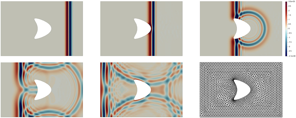
Figure 3. Computational mesh of the rectangular domain Ω with an obstacle (second row, right) used for all the computation. The first row and second (left and middle) show snapshots at t = 0, 2, 4, 6, 8 of the velocity variables vh approximated by the Hamiltonian HDG method (Equation 13) with polynomial approximation spaces of order 3 and the implicit midpoint.
In Figure 3, we present the computational mesh of the domain used in our computations. We compare six numerical schemes:
• CG-symp: Continuous Galerkin with polynomial order 3, and implicit midpoint scheme (symplectic).
• CG-diss: Continuous Galerkin with polynomial order 3 and singly DIRK method of order 3 (nonsymplectic), see Table 5.
• Mixed-symp: Mixed method with Raviart-Thomas spaces of order 3, and Störmer-Verlet scheme (symplectic PRK method of order 2).
• Mixed-diss: Mixed method with Raviart-Thomas spaces of order 3 and singly DIRK method of order 3 (nonsymplectic), see Table 5.
• HDG-symp: Hamiltonian HDG method (Equation 13) with polynomial order 3, and implicit midpoint scheme (symplectic).
• HDG-diss: HDG method (Equation 12) (non-Hamiltonian) with polynomial order 3, and implicit midpoint scheme (symplectic).
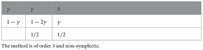
Table 5. Butcher array for a singly diagonally implicit Runge-Kutta method, with .
We illustrate the evolution of the numerical approximation given by the Hamiltonian HDG method with polynomial approximations of order 3 and implicit midpoint in Figure 3. Snapshots are presented at times t = 0, 2, 4, 6, 8.
In Figure 4 we present a comparison of the numerical schemes computing the physical quantities energy (see Table 1), linear momentum, and the norm of the pseudomomentum for the six methods. In the first column, we plot the energy loss, that is, , for the energy computed with each numerical scheme at the time tn. In the second column, we plot the linear momentum loss and, in the third column the evolution of the pseudomomentum. We observe the improved approximation of the energy and pseudomomentum of the symplectic Hamiltonian finite element methods. The linear momentum, which is a first integral of the system, is preserved for each of the numerical schemes.
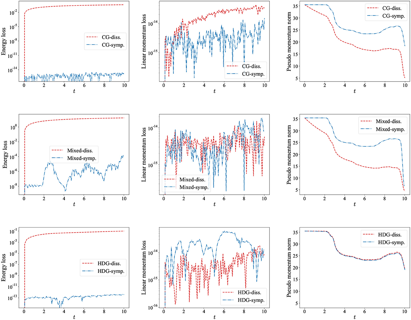
Figure 4. Plots of the approximated physical quantities: Energy loss (left), linear momentum loss (middle), and pseudomomentum. The first row shows a comparison of the continuous Galerkin methods using the implicit midpoint (dot-dashed blue line) and an sDIRK method of order 3 (dashed red line). The second row shows a comparison of the Mixed method using the Raviart-Thomas element with a polynomial approximation of order 3, using the Störmer-Verlet scheme and the sDIRK method of order 3. The third row shows a comparison of the Hamiltonian HDG scheme (Equation 13) and the dissipative HDG scheme (Equation 12), for both we use the implicit midpoint.
6. Ongoing work
As we have seen, the application of a symplectic time-marching method to a Hamiltonian system of ODEs can guarantee the preservation of all its linear and quadratic invariants. On the other hand, to obtain such a system of ODEs, one uses space discretizations which do not guarantee the preservation of all the linear and quadratic invariants of the original Hamiltonian PDEs! Indeed, as far as we can tell, it is not well understood how to obtain all the discrete versions of those invariants for any given space discretization, by finite difference or finite element methods. In fact, although it is almost automatic how to find discrete versions of the energy, the discrete equivalents of other conserved quantities, like the Lipkin's invariants for electromagnetism, for example, remain elusive. This topic constitutes the subject of ongoing work.
Recently, a new class of symplectic Discontinuous Galerkin methods were found whose distinctive feature is the use of time operators for defining their numerical traces, see Cockburn et al. [9]. Work to find how useful this type of methods are is under way.
The combination of Galerkin space discretizations with symplectic time-marching methods to a variety of systems of nonlinear Hamiltonian problems, including the Schrödinger and KdV equations, finite deformation elasticity, water waves and nonlinear wave equations, is also the subject of ongoing work.
Author contributions
All authors listed have made a substantial, direct, and intellectual contribution to the work and approved it for publication.
Funding
BC was supported in part by the NSF through grant no. DMS-1912646. MS was partially supported by FONDECYT Regular grant no. 1221189 and by Centro Nacional de Inteligencia Artificial CENIA, FB210017, Basal ANID Chile.
Acknowledgments
The authors would like to express their gratitude to EC for the invitation to write this article. The authors also want to thank Peter Olver for many useful clarifications on the various concepts used for the systems under consideration and for bringing to their attention the Olver [5, Example 4.36] and Walter [32] about conservation laws for the scalar wave equation.
Conflict of interest
The authors declare that the research was conducted in the absence of any commercial or financial relationships that could be construed as a potential conflict of interest.
Publisher's note
All claims expressed in this article are solely those of the authors and do not necessarily represent those of their affiliated organizations, or those of the publisher, the editors and the reviewers. Any product that may be evaluated in this article, or claim that may be made by its manufacturer, is not guaranteed or endorsed by the publisher.
Footnotes
1. ^What we are denoting by J was originally denoted by J−1. We decided not to keep such notation because it suggests the invertibility of J and this property does not hold in many interesting cases. For example, when extending these definitions from ODEs to PDEs, J−1 naturally becomes a non-invertible differential operator, as already noted in the pioneering 1988 work by Ge and Feng [10, Section 3]. This prompted them to simply drop the notation J−1. No wonder most authors dealing with Hamiltonian PDEs, see, for example, the 1993 book by Olver [5], automatically replace the original J−1 by J, just as we are doing it here.
2. ^This holds when the functional only depends on the phase variable u. If the functional depends also on time, that is, if , the above calculation must be modified to read .
3. ^This generalization is so simple that, in our first reading, the difference between a “Hamiltonian” and a “Poisson” dynamical system completely escaped us.
4. ^A small remark on the matrix A: = JH is in order. For the canonical structure matrix J, it is standard to say that the matrix A is Hamiltonian if J⊤A = H is symmetric. If J is only required to be invertible, one could say that A is a Hamiltonian matrix if J−1A = H is symmetric. Finally, if J is not invertible, one is tempted to say that A is a “Poissonian” matrix if AJ = JHJ is symmetric. We did not find this terminology in the current literature and so dissuaded ourselves to introduce it here, especially because we do not need it in a significant way.
5. ^This is an example of a Casimir: a function C whose gradient ∇C lies in the kernel of J. The functional C is then conserved for any Poisson system with structure matrix J. A Casimir is also called a distinguished function in the 1993 book by Olver [5]. The history of the term Casimir can be found in the notes to Chapter 6 of that book.
6. ^In the framework of PDEs, the fine distinction made between “Hamiltonian” and “Poisson” dynamical systems of ODEs does not seem too popular. In the 2006 book by Harier et al. [14, Section VII.2], a “Poisson” dynamical system is defined as the dynamical system obtained when (in our notation) the structure matrix J is a non-constant matrix which depends on the unknown u, J = J(u). We were perplexed by the explicit absence of the case in which J is constant but not necessarily invertible. However, later we understood that the “constant” case was trivially contained in the more interesting “non-constant” one.
7. ^Everything done for the scalar wave equation can be extended to the equations of elastodynamics very easily. See, for example, the Hamiltonian formulations in our recent work [2] and the six independent conservation laws in the 1976 work by Fletcher [20].
8. ^For a geometric interpretation of the symplecticity of an operator, see the 1992 review by Sanz-Serna [13], the 2006 book by Hairer et al. [14] and the 2010 book by Feng and Qin [8]. In the many discussions with our dynamical system colleagues, we always got the impression that symplecticity enhances the numerical schemes in much better ways than the simple conservation of energy can. We admit that we are more ready to believe their statements than to really understand their arguments. Perhaps because it is difficult to visualize orbits of infinite-dimensional dynamical systems. To be pragmatic, we restrict ourselves to the operational definition of symplecticity given by equality (b).
9. ^To us, the intuition of what is a Poisson integrator matrix can be extracted directly from Proposition 3.2: If the matrix A is of the form JH, with J anti-symmetric and H symmetric, then the matrix etA is a Poisson integrator matrix. We have the impression that the properties defining Poisson integrator matrices can be formulated precisely to match this remarkable relation.
References
1. SánchezMA, Ciuca C, Nguyen NC, Peraire J, Cockburn B. Symplectic Hamiltonian HDG methods for wave propagation phenomena. J Comput Phys. (2017) 350:951–73. doi: 10.1016/j.jcp.2017.09.010
2. SánchezMA, Cockburn B, Nguyen NC, Peraire J. Symplectic Hamiltonian finite element methods for linear elastodynamics. Comput Methods Appl Mech Engrg. (2021) 381:113843. doi: 10.1016/j.cma.2021.113843
3. SánchezMA, Du S, Cockburn B, Nguyen NC, Peraire J. Symplectic Hamiltonian finite element methods for electromagnetics. Comput Methods Appl Mech Engrg. (2022) 396:114969. doi: 10.1016/j.cma.2022.114969
4. Fu G, Shu CW. Optimal energy-conserving discontinuous Galerkin methods for linear symmetric hyperbolic systems. J Comput Phys. (2019) 394:329–63. doi: 10.1016/j.jcp.2019.05.050
5. Olver PJ. Applications of Lie Groups to Differential Equations. Vol. 107 of Graduate Texts in Mathematics. 2nd ed. New York, NY: Springer-Verlag (1993).
6. Marsden JE, Ratiu TS. Introduction to Mechanics and Symmetry. Vol. 17 of Texts in Applied Mathematics. 2nd ed. New York, NY: Springer-Verlag (1999).
7. Leimkuhler B, Reich S. Simulating Hamiltonian Dynamics. Vol. 14 of Cambridge Monographs on Applied and Computational Mathematics. Cambridge: Cambridge University Press (2004).
8. Feng K, Qin MZ. Symplectic geometric algorithms for Hamiltonian systems. In: Zhejiang Science and Technology Publishing House, Hangzhou: Springer, Heidelberg; (2010).
9. Cockburn B, Du S, Sánchez MA. Discontinuous Galerkin methods with time-operators in their numerical traces for time-dependent electromagnetics. Comput Methods Appl Math. (2022) 22:775–96. doi: 10.1515/cmam-2021-0215
10. Ge Z, Feng K. On the Approximations of linear Hamiltonian systems. J Comput Math. (1988) 6:88–97.
11. Feng K, Qin MZ. The symplectic methods for the computation of Hamiltonian equations. In: Numerical methods for partial differential equations (Shanghai, 1987). vol. 1297 of Lecture Notes in Math. Berlin: Springer (1987). p. 1–37.
12. Feng K, Wu HM, Z M. Symplectic difference schemes for linear Hamiltonian systems. J Comput Math. (1990) 8:371–80.
13. Sanz-Serna JM. Symplectic integrators for Hamiltonian problems: an overview. In: Acta Numerica 1992 Acta Numer. Cambridge: Cambridge Univ. Press (1992). p. 243–86.
14. Hairer E, Lubich C, Wanner G. Geometric numerical integration : structure-preserving algorithms for ordinary differential equations. In: Springer Series in Computational Mathematics. Berlin; Heidelberg; New York, NY: Springer. (2006).
15. Yee K. Numerical solution of initial boundary value problems involving Maxwell's equations in isotropic media. IEEE Trans Antennas Propagat. (1966) 14:302–7. doi: 10.1109/TAP.1966.1138693
16. McLachlan R. Symplectic integration of Hamiltonian wave equations. Numer Math. (1993) 66:465–92. doi: 10.1007/BF01385708
17. Groß M, Betsch P, Steinmann P. Conservation properties of a time FE method. Part IV: Higher order energy and momentum conserving schemes. Internat J Numer Methods Engrg. (2005) 63:1849–97. doi: 10.1002/nme.1339
18. Xu Y, van der Vegt JJW, Bokhove O. Discontinuous Hamiltonian finite element method for linear hyperbolic systems. J Sci Comput. (2008) 35:241–65. doi: 10.1007/s10915-008-9191-y
19. Kirby RC, Kieu TT. Symplectic-mixed finite element approximation of linear acoustic wave equations. Numer Math. (2015) 130:257–91. doi: 10.1007/s00211-014-0667-4
20. Fletcher DC. Conservation laws in linear elastodynamics. Arch Rational Mech Anal. (1976) 60:329–53. doi: 10.1007/BF00248884
21. Lipkin DM. Existence of a new conservation law in electromagnetic theory. J Math Phys. (1964) 5:695–700. doi: 10.1063/1.1704165
22. Tang Y, Cohen AE. Optical chirality and its interaction with matter. Phys Rev Lett. (2010) 104:163901. doi: 10.1103/PhysRevLett.104.163901
23. Yoshida H. Construction of higher order symplectic integrators. Phys Lett A. (1990) 150:262–8. doi: 10.1016/0375-9601(90)90092-3
24. Bridges JT, Reich S. Numerical methods for Hamiltonian PDEs. J Phys A. (2006) 39:5287–320. doi: 10.1088/0305-4470/39/19/S02
25. Taflove A. Application of the finite-difference time-domain method to sinusoidal steady-state electromagnetic-penetration problems. IEEE Trans Electromagn Compatibil. (1980) 3:191–202. doi: 10.1109/TEMC.1980.303879
26. Sun Y, Tse PSP. Symplectic and multisymplectic numerical methods for Maxwell's equations. J Comput Phys. (2011) 230:2076–94. doi: 10.1016/j.jcp.2010.12.006
27. Stern A, Tong Y, Desbrun M, Marsden JE. Geometric computational electrodynamics with variational integrators and discrete differential forms. In: Geometry, Mechanics, and Dynamics. vol. 73 of Fields Inst. Commun. New York, NY: Springer (2015). p. 437–75.
28. Cockburn B, Fu Z, Hungria A, Ji L, Sánchez MA, Sayas FJ. Stormer-Numerov HDG methods for acoustic waves. J Sci Comput. (2018) 75:597–624. doi: 10.1007/s10915-017-0547-z
29. Nguyen NC, Peraire J, Cockburn B. High-order implicit hybridizable discontinuous Galerkin methods for acoustics and elastodynamics. J Comput Phys. (2011) 230:3695–718. doi: 10.1016/j.jcp.2011.01.035
30. Cockburn B, Quenneville-Bélair V. Uniform-in-time superconvergence of HDG methods for the acoustic wave equation. Math Comp. (2014) 83:65–85. doi: 10.1090/S0025-5718-2013-02743-3
31. Hairer E, Wanner G. Solving ordinary differential equations. II, volume 14 of Springer Series in Computational Mathematics. 2nd ed. Berlin: Springer-Verlag (1996).
32. Walter AS. Nonlinear invariant wave equations. In: Invariant Wave Equations (Proc. Ettore Majorana International School of Mathematical Physics Erice, 1977), Lecture Notes in Physics, Vol. 73. Berlin: Springer (1978). p. 197–249.
33. Anco SC, Pohjanpelto J. Classification of local conservation laws of Maxwell's equations. Acta Appl. Math. (2001) 69:285–327. doi: 10.1023/A:1014263903283
Appendix
1. Symplectic partitioned Runge-Kutta methods
Here, we provide a proof of Proposition 3.8 which characterizes the Symplectic Partitioned Runge-Kutta (PRK) methods for ODEs. We use the notation of Section 3.4.
We must show that is zero for any u1 and u2 in ℝd. By Theorem 3.3, for any element v of the kernel of J. Thus, we can take u1 and u2 in the range of J. On that subspace, J is invertible and it is enough to prove that is zero.
Inserting the definition of the PRK numerical method EΔt, we obtain
because A = JH. Since we get that
and so
where
Next, we incorporate the information of the Hamiltonian being separable:
and, with , conclude that
by hypothesis. This completes the proof of Proposition 3.8.
Keywords: symplectic time-marching methods, finite difference methods, finite element methods, Hamiltonian systems, Poisson systems
Citation: Cockburn B, Du S and Sánchez MA (2023) Combining finite element space-discretizations with symplectic time-marching schemes for linear Hamiltonian systems. Front. Appl. Math. Stat. 9:1165371. doi: 10.3389/fams.2023.1165371
Received: 14 February 2023; Accepted: 14 March 2023;
Published: 05 April 2023.
Edited by:
Eric Chung, The Chinese University of Hong Kong, ChinaReviewed by:
Guosheng Fu, University of Notre Dame, United StatesLina Zhao, City University of Hong Kong, Hong Kong SAR, China
Yanlai Chen, University of Massachusetts Dartmouth, United States
Copyright © 2023 Cockburn, Du and Sánchez. This is an open-access article distributed under the terms of the Creative Commons Attribution License (CC BY). The use, distribution or reproduction in other forums is permitted, provided the original author(s) and the copyright owner(s) are credited and that the original publication in this journal is cited, in accordance with accepted academic practice. No use, distribution or reproduction is permitted which does not comply with these terms.
*Correspondence: Bernardo Cockburn, YmNvY2tidXJAdW1uLmVkdQ==