 Jorin Dornemann
- Institute of Mathematics, Hamburg University of Technology, Hamburg, Germany
Vehicle routing problems are a class of NP-hard combinatorial optimization problems which attract a lot of attention, as they have many practical applications. In recent years there have been new developments solving vehicle routing problems with the help of machine learning, since learning how to automatically solve optimization problems has the potential to provide a big leap in optimization technology. Prior work on solving vehicle routing problems using machine learning has mainly focused on auto-regressive models, which are connected to high computational costs when combined with classical exact search methods as the model has to be evaluated in every search step. This paper proposes a new method for approximately solving the capacitated vehicle routing problem with time windows (CVRPTW) via a supervised deep learning-based approach in a non-autoregressive manner. The model uses a deep neural network to assist finding solutions by providing a probability distribution which is used to guide a tree search, resulting in a machine learning assisted heuristic. The model is built upon a new neural network architecture, called graph convolutional network, which is particularly suited for deep learning tasks. Furthermore, a new formulation for the CVRPTW in form of a quadratic unconstrained binary optimization (QUBO) problem is presented and solved via quantum-inspired computing in cooperation with Fujitsu, where a learned problem reduction based upon the proposed neural network is applied to circumvent limitations concerning the usage of quantum computing for large problem instances. Computational results show that the proposed models perform very well on small and medium sized instances compared to state-of-the-art solution methods in terms of computational costs and solution quality, and outperform commercial solvers for large instances.
1. Introduction
The capacitated vehicle routing problem with time windows (CVRPTW) is a well-known combinatorial optimization problem that arises in a variety of practical contexts, including delivery scheduling, emergency response planning, and supply chain management. In the CVRPTW, a fleet of vehicles must be routed to deliver goods to a set of customers, subject to capacity constraints and time window constraints, which specify the allowable time periods for the deliveries to be made. Finding the optimal routes for the vehicles is a challenging problem, as it involves balancing the conflicting objectives of minimizing the total distance traveled and maximizing the number of deliveries that can be made within the time window constraints.
Over the years, a wide range of solution approaches have been proposed for the CVRPTW, including exact algorithms, such as branch-and-cut and branch-and-price [1], and heuristics, such as genetic algorithms, simulated annealing, and tabu search [2]. These methods differ in their complexity and the quality of the solutions they produce. In recent years, there has been a growing interest in developing approximate algorithms for the CVRPTW, as these methods can scale to large-sized instances and produce high-quality solutions in reasonable time. Examples of such algorithms include the adaptive large neighborhood search and the variable neighborhood search [3, 4].
Heuristics for routing problems can be divided into two categories: construction heuristics and improvement heuristics [1]. Similarly, machine learning-based methods for solving routing problems also feature these characteristics. Some approaches, such as those in [5] and [6], focus on iteratively improving an existing solution, while others, such as those developed by [7], [8], and [9] generate a solution for the CVRP by adding one node at a time. Improvement approaches typically rely on an initial solution that they can then refine over time. However, it may be challenging to find a suitable starting solution for more complex problems like the CVRPTW. In fact, finding a first feasible solution for the CVRPTW with a fixed number of vehicles is an NP-hard problem on its own [10]. Furthermore, improvement approaches often require multiple iterations to arrive at good solutions, and the number of iterations required tends to escalate with an increase in problem complexity. This non-linear relationship between problem size and iteration count implies that more complex problems require substantially greater computational resources to attain optimal solutions using iterative improvement methods. On the other hand, constructive methods can generate solutions within a set number of steps that is linearly dependent on the size of the problem. But the limited information available about the other tours while constructing new tours node by node can lead to inefficient constructions and obtaining additional information in the space of solutions that are constructed sequentially becomes expensive quickly.
Moreover, there has been a surge of interest in quantum computers and the potential they hold for solving complex optimization problems, that are beyond the capabilities of classical computers. Quantum computers have the ability to perform certain types of optimization tasks much faster and more efficiently than classical computers. As quantum computers might become more advanced and accessible in the nearer future, the development of models for optimization problems that can take advantage of their unique capabilities becomes increasingly relevant.
Our goal in this work is to merge the latest advances in deep learning techniques for routing problems with quantum computing. We do this by adapting the work of [11] for the CVRPTW and creating a constructive heuristic for the CVRPTW that utilizes a deep learning model. We then proceed by developing a novel formulation of the CVRPTW as a quadratic unconstrained binary optimization problem and derive a binary quadratic program from this formulation. We then use the deep learning model as a form of learned problem reduction [12] to reduce the problem instances to a size that can be handled by quantum-inspired computers from Fujitsu and conduct computational experiments for both approaches. We show that our constructive deep learning heuristic model outperforms commercial state-of-the-art solvers such as Gurobi [13] for larger instance sizes for the CVRPTW, while being close to competitive with the highly-optimized LKH heuristic [14] and Google's OR-Tools [15] on smaller instances in terms of solution quality, showing the power deep learning has to handle difficult constraints such as time windows. But for large instances a shortcoming of the constructive nature of the model becomes apparent, as the very limited information on which the next decision is based prevents finding the best solutions. Our quadratic unconstrained binary optimization model, which is solved through quantum-inspired computing, aims at overcoming some of these challenges due to its non-constructive nature. Our results show the potential that the combination of deep learning and quantum computing holds.
The remaining paper is organized as follows: In Section 2, a comprehensive overview of related work on constructive approaches for solving the CVRPTW and variants using deep learning tools is provided. The proposed models are described in detail in Section 3. In Section 4, the computational results obtained from the developed models are presented and discussed. A summary of the results and an outlook for future research is given in Section 5.
2. Related work
Building on the work of [16], who introduced the Pointer Network (PtrNet), which is a deep neural network that uses attention to output a permutation of the input and was trained in a supervised way to solve the Traveling Salesman Problem (TSP), many improvements for this constructive approach have been proposed. An extension to reinforcement learning for using the PtrNet to solve TSPs was proposed by [17]. Nazari et al. [7] adapted this for the CVRP, but replaced the recurrent neural network part [18] of the encoder by a linear embedding layer with shared parameters. Reinforcement learning as the training strategy was also pursued in various other models for TSP variants [19–21] as well as for the CVRP [8, 20, 22, 23], since supervised learning approaches depend on the availability of large sets of high-quality solutions, as noted in [24]. One commonality among these constructive methods is that they are auto-regressive, which means the model must be evaluated every time a new node is added to the tour.
Unlike these auto-regressive methods, Joshi et al. [11] used supervised learning to train a graph neural network to produce a tour for the TSP in the form of an adjacency matrix. This matrix is then converted into a feasible solution for the TSP using beam search, a limited-width breadth-first search [25]. They build on the work of [26], who followed a similar approach to approximately solve the TSP by using a graph neural network [27], but their model performed poorly even on smaller instances. Instead of using graph neural networks, Joshi et al. [11] use deep graph ConvNets [28], which are graph convolutional neural networks that are able to learn from larger training sets, and were able to outperform all other learning-based approaches for the TSP. This outcome is unsurprising since supervised learning techniques tend to perform better than reinforcement learning techniques when enough training data is available. Our approach builds on the work of [11].
However, incorporating time window constraints is a difficult task, and there have been only a few recent proposals for constructive approaches to the CVRPTW that utilize deep learning. The first constructive method using deep learning for the CVRPTW was proposed by [9]. They use the attention model from [8] for the CVRP, which constructs one route at a time by treating all not yet visited nodes as actions and learning a policy model to choose the next node via reinforcement learning. Falkner and Schmidt-Thieme [9] extend this approach for the CVRPTW by constructing multiple routes simultaneously and using the information of all partially constructed routes to choose the next node. Although the computational results of this model are promising, it is computationally intensive to use. Furthermore, their main objective is not to minimize the total distance traveled, but a combination of total distance traveled, waiting times for the vehicles and number of vehicles used as well as also considering soft time windows, where violating time window constraints is penalized rather than forbidden, but through appropriate weighting the objective function could be adjusted to focus on one goal. Falkner et al. [29] extend the work of [9] by replacing the self-attention layers of their model by graph neural networks to encode the problem and propose a Large Neighborhood Search using a learned construction heuristic via reinforcement learning to re-construct partially destructed solutions in an auto-regressive manner. A hierarchical reinforcement learning model based on pointer networks was proposed by [30]. This model involves learning to obtain feasible solutions at a lower level and using these solutions as input for a second decoder to minimize the total distance. However, this approach is only effective for relatively small numbers of customers. Two improvement-based methods for the CVRPTW have been proposed recently. The first one by [31] uses an enhanced version of the graph attention network [32] to learn a heuristic for Very Large-scale Neighborhood Search that includes both improvement and destruction operators. They are able to approximately solve instances with up to 400 nodes, with respect to standard heuristics the improvements in terms of solution quality are at around 4–5 %. Silva et al. [33] propose a reinforcement learning-based model that learns eight different neighborhood functions for a Variable Neighborhood Descent heuristic with tabular Q-learning.
Exact solution methods for the CVRPTW can be divided into three categories according to [1]: Branch and Cut and Price, Branch and Cut, and reduced set partitioning. Most successful algorithms have been based on column generation, where the problem is decomposed into a restricted master problem that selects new routes from a subset of candidate routes and a pricing subproblem that generates new routes to be considered in the restricted master problem. In general, the pricing subproblem obtained is a shortest path problem with resource constraint (SPPRC) [34] which is NP-hard [35]. To obtain better lower bounds in the Branch and Bound search tree different methods have been proposed. Kohl et al. [36] proposed adding valid inequalities dynamically to strengthen linear relaxations, which results in a Branch and Cut and Price algorithm. Other families of inequalities were subsequently proposed over the years [37–39]. Other approaches aim at strengthening the pricing subproblem by using algorithms to generate new routes which include labeling algorithms [34, 40, 41] and heuristics [2, 42], but solving the SPPRC exactly remains an obstacle. Baldacci et al. [43] therefore developed a different relaxation approach for the pricing subproblem, where a set partitioning formulation is used in which routes are dynamically generated via column generation. Their algorithm can be seen as a three-step method, where calculated lower and upper bounds are used to enumerate a subset of all feasible routes whose reduced cost with respect to the dual solution is less than or equal to the gap between the lower and upper bound. Afterwards the CVRPTW is formulated as a mixed integer program (MIP), where the previously determined subset of feasible solutions is incorporated, and solved using a commercial MIP solver. For an extensive review of all exact solution approaches, we refer to the surveys of [44] and [1].
To the best of our knowledge, the combination of quadratic unconstrained binary optimization with techniques from deep learning to solve combinatorial problems has not yet been proposed. Just recently, [45] and [46] proposed unconstrained binary models for variants of the TSP. We refer to [47] for an overview of quadratic unconstrained binary optimization for routing problems. Bengio et al. [24] present a recent survey on combinatorial optimization with machine learning techniques.
3. Problem setting and model
The purpose of this chapter is to provide a comprehensive introduction to the CVRPTW, along with a detailed explanation of the design of the deep neural network. Furthermore, we present two distinct methods for constructing solutions and elaborate on how the information obtained from the network is utilized in both approaches.
3.1. Problem setting
The Capacitated Vehicle Routing Problem with Time Windows (CVRPTW) is an extension of the classical and best known routing problem, the Traveling Salesman Problem (TSP). Given a fleet of K vehicles, the goal is to find routes, such that all nodes are visited and the capacity and time window constraints are met.
More specifically, a CVRPTW instance is given as a directed fully connected graph G = (V, E) with n+1 nodes, where node 0 is the special depot node. The cost for edge e = (i, j) is given by cij and represents the transit costs from node i to j. Besides its coordinates, each node has additional attributes, namely a demand and a time window, imposing conditional constraints on the nodes. Therefore, we can define a problem instance of the CVRPTW to consist of:
• X = {x1, …, xn}, where are the coordinates of node i in the two-dimensional unit square.
• The location of the depot, given as .
• The demands at each node i∈[n], given as D = {d1, …, dn}.
• T = {[a0, b0], [a1, b1], …, [an, bn]}, where [ai, bi] are the time windows for each node i∈[n] and [a0, b0] represents the planning horizon regarding earliest possible departure from and latest possible return to the depot.
• The capacity of the vehicles C.
Moreover each node i∈V requires a specific service duration hi. The aim is to find routes rk, k∈[K], such that all nodes are visited. A tour rk is a sequence of nodes, starting and ending at the depot node 0, representing the order in which vehicle k visits the nodes. A set of tours R = {r1, …, rK} is considered a solution, if ∪k∈[K]rk = V, ∩k∈[K]rk = {0} and all tours satisfy the capacity and time window constraints. The capacity constraint is given as C and the time window constraint states, that the time service starts at node i, si, has to satisfy ai ≤ si ≤ bi. An arrival at node i before ai is considered valid, the vehicle then has to wait until ai to start the service.
The components of the instances contain a few assumptions. We assume a homogenous fleet of K vehicles, so that the capacity and travel time is equal for all vehicles. Furthermore, the edge weights cij represent the transit costs from node i to node j and without loss of generality include the service durations hi of node i.
There are different approaches to formulate the objective function. The classical objective function is to minimize the total distance traveled over all vehicles. But there are more advanced formulations of the objective, for example [9] take a more holistic perspective by also including the waiting times into the objective, searching for a good trade-off between total distance, waiting times and number of vehicles. On the other hand, especially in the operations research literature, the main objective is to minimize the number of vehicles, including the total distance just as a secondary, which has its source in cost reduction being the main focus. Other objectives include minimizing the total distance traveled while using all K vehicles (see [48]). In this work, we focus on the classical approach by minimizing the total distance, but pursuing other objectives would only need small changes in our models.
3.2. Graph convolutional network
For our model we use a graph neural network called Residual Gated Graph ConvNet (GCN) (see [28]), which was adapted for the TSP in [11]. They provide a framework to solve routing problems using the GCN, however, they only adapt it to solve the TSP with no consideration of time windows. In this section, we present our extension to address the CVRPTW, which relies on modifying the layers to adapt additional constraints within the framework and modify the search method for constructing full solutions.
The neural network outputs probabilities over the edges of the graph in order to predict which edges are most promising to be included in a solution. Complete solutions are obtained by converting these probabilities received from the model to valid tours via beam search [25], straightforward heuristics or quantum-inspired computing.
3.2.1. Input layer
The input for the node features is five-dimensional. For node i we have the two-dimensional coordinates , the time window given as [ai, bi] and the normalized demand di/C, where we set d0 = 0 for the depot. These features are concatenated to the five-dimensional input feature vector yi and are then embedded to a -dimensional representation , where h denotes the hidden dimension of our network. Similar to [49], the special depot node gets a separate learned initial embedding parameter. For that, define to be the unit vector with entry one at the first position and zeros otherwise. This is put together as the node input feature as follows:
where , and ·⊕· is the concatenation operator.
For the input edge feature, the edge values cij are embedded as a -dimensional feature vector. We do not integrate the K-nearest neighbor feature used in [11], since, in contrast to the TSP without time windows, the assumption that a node in the solution is usually connected to nodes in its close proximity (see [11]) does not necessarily hold with time window constraints. Instead, we use an indicator function δij of an edge which has the value one for edges connecting nodes i and j, with i≠j and i, j not the depot, and value two for edges connecting nodes with itself. To tag the depot as a special node, the indicator function δij furthermore has value 3 for edges to and from the depot and value 4 for the depot self-loop. Together, the edge input feature is given as:
where and . As for the parameters A2, we apply a separate embedding layer to learn the embedding parameters A4 for our indicator function δij.
3.2.2. Graph convolution layer
In each of the Graph Convolution layers the model updates the edge and node embeddings. Following [11], we leverage the design of the Residual Gated Graph ConvNet developed in [28] by adding an edge feature representation. Let ℓ be the current layer and for node i and edge (i, j), let be the node features vector and the edge features vector. We define the features for layer ℓ+1 in the following way:
where for k∈[5], σ is the sigmoid function, ε is a small value, ReLU being the rectified linear unit, BN stands for batch normalization, N(i) denotes the neighborhood of node i, ·⊙· denotes the Hadamard product operator and being defined as
For the input layer, we set and . We implement as a separate parameter in order to allow the model to distinguish different directions of edges, since in the context of CVRPTW we have directed edges in our solutions. The training labels for the edges are also set accordingly, meaning if edge (i, j) is contained in the solution, then edge (j, i) will have label zero, although edge (i, j) is labeled with a one (see [49]). Batch normalization is a mechanism that normalizes layer inputs in order to reduce internal covariate shifts which allows the usage of higher learning rates and hence accelerates the learning of deep architectures (see [50] for more details).
3.2.3. MLP classifier
A Multi-layer Perceptron (MLP), which is a fully connected feedforward neural network with a number ℓC of hidden layers, is used for generating the desired output, a finite measure that represents probabilities over the edges of our fully connected graph. For each edge embedding of the last Graph Convolution layer L, the MLP outputs the probability pij that this edge is included in the tours of the CVRPTW solution:
The edge representations are linked to the ground-truth tour through a softmax output layer, which allows us to train the model parameters end-to-end by minimizing the cross-entropy loss via gradient descent (see [11]).
In the following sections, we describe two methods which use these edge probabilities to build valid solutions.
3.3. Beam search
To create valid solutions from our network model's output, we cannot simply select the edges with the highest probability until all nodes are visited, as this often results in invalid tours. Instead, we use beam search [25], a limited-width breadth-first tree search, to construct solutions.
Starting from the root node (which may be the depot but can also contain an initial partial solution), in each layer of the search tree, only a subset of the nodes with regard to a scoring policy are further explored. The descendants of a node i in layer ℓ are those nodes that are eligible as the next stop for the partially constructed tour represented in i. In the context of CVRPTW, where we have dynamic parts of partial solutions, such as the current point of time and the already occupied capacity of the vehicle, we apply a masking strategy to efficiently build valid solutions. This is done by masking out invalid descendants in layer ℓ+1 with respect to the time window and demand constraints as well as the already visited nodes in this partial solution. Then, from the set of all nodes in layer ℓ+1, only a subset containing the b best nodes (with respect to the scoring function) are retained, the other nodes are discarded. The parameter b is called the beam width. In our case, the scoring function are the probabilities gained by the GCN and we choose the b nodes whose connecting edges hold the highest probability. This is done iteratively, until all nodes in the graph are visited. If a node contains a full solution, the solution is evaluated and stored. The beam search stops when no more branches are possible on the current level, i.e., when b complete solutions have been found. The final solution then is the one which yields the highest score with respect to the scoring function, which translates to having the highest probability out of the b found solutions regarding the output of our neural network.
Beam search is asymptotically optimal for b = n·2n, but choosing a smaller b allows us to trade quality for computational performance and memory needed, since it decreases the search space but possibly the best solution is pruned. Furthermore, the beam search can take a sparse graph instead of a fully connected graph as an input to accelerate the tree search. This enables us to utilize the neural network in a second manner, as we can set a threshold to the edge probability given by the neural network for an edge to be included in the sparse graph, which is then given as input for the beam search. This can be interpreted as a learned problem reduction [12]. We use a low threshold of at least 10−4, which already excludes most of the edges. For details about the reduction see Section 4.3.1.
The approach of choosing the solution with the highest probability produced by the beam search is called GCNBS in the following. However, out of the b solutions found, we can also select the one having the overall shortest tour. This follows the approach in [17], where they sample a set of solutions and select the shortest one as the final solution out of this set, and can be interpreted as a shortest tour heuristic [11], which is therefore called GCNBSSTH in the rest of the paper.
3.4. Quadratic unconstrained binary optimization
In this section, we present a second approach to build feasible solutions to the CVRPTW using our proposed neural network model. In recent years, the development in quantum technologies led to bigger interest in formulating combinatorial optimization as quadratic unconstrained binary optimization problems (QUBO), as these formulations are suited best to be solved via quantum computing (see [47]). The CVRPTW imposes time window constraints, which are expressed as inequality constraints. Generally speaking, inequalities are known to be particularly difficult to handle within QUBO models (see [45]).
Building on the work of [46], we develop a new formulation for the CVRPTW as an quadratic unconstrained binary optimization problem. We work with an integer linear programming (ILP) formulation based on edge presentations as a starting point, as this approach is best suited to benefit from our learning-based problem reduction presented in Section 3.2. We derive a novel QUBO formulation for the CVRPTW and asymptotically calculate the number of variables needed to model this formulation. From this QUBO formulation, we derive a binary quadratic program (BQP), which is then used to solve the CVRPTW on hardware specialized for solving BQPs and QUBO problems. We use the BQP because it allows us to solve larger problem instances on said hardware. This is explained in detail in Section 3.4.5.
3.4.1. Introduction to QUBO
Oftentimes, optimization problems can be formulated as finding the minimum of a function f which models problem p. The global minimum of f represents the optimal solution of p. Quadratic unconstrained binary optimization aims at formulating optimization problems as quadratic polynomials, where the decision variables are binary. In detail, a QUBO problem is of the form
where x is our decision vector containing the binary decision variables and Q is a square upper-triangular matrix taking values in the reals. The goal is to find the vector x* that minimizes f. This general form includes quadratic as well as linear objective functions, if Q is a diagonal matrix and one notices that for xi∈{0, 1}.
A more comprehensive introduction into QUBO can be found in [51].
3.4.2. General approach from ILP to QUBO
In general, given an ILP problem of the form
where ai, b∈ℝ, we can obtain a QUBO formulation by transforming the equality constraints into the objective function:
obtaining a new function which is equal to the original ILP if and only if the binary decision variables zi fulfill the equality constraint. The value for the penalty constant P∈ℝ≥0 has to be set to weigh the constraints. Now, lets assume we are given an ILP problem, where the variables zi are not binary, but rather integer variables with bounds . Since a QUBO problem is only able to handle binary variables, we have to convert the integer variables to binary by replacing each z with its binary expansion:
where and xz, j are new binary variables. If linear inequality constraints are given of the form
they must be converted into equality constraints by adding slack variables λ to derive . These additional integer slack variables also have to be optimized, resulting in a larger representation of the original problem after applying the binary expansion (9). In order to bound the number of additional variables needed, we can define sharp upper and lower limits for the value the slack variables can take. Generally speaking, it holds that
but problem specific knowledge oftentimes allows to find sharper bounds.
3.4.3. ILP formulation of the CVRPTW
Given the directed graph G = (V, E), with V = {0, …, n} and 0 being the depot, and a fleet of K vehicles each with a capacity of C, let the decision variables xi, j for i, j∈V, with i≠j, be defined as
Note that in order to minimize the number of decision variables needed, the point in time in which the edge is used is not specified with the decision variable. To model the time window constraints, let the variable si represent the time at which the vehicle arrives at node i. Each node i∈[n] has an associated time window [ai, bi] and demand di and the edge costs representing the travel time between nodes is given as cij for edge (i, j). Let yi be the available capacity of the vehicle after visiting node i∈[n]. The ILP for the CVRPTW can be formulated as follows:
where (13) are the assignment constraints requiring each customer to be served by exactly one vehicle (note that the depot is excepted), (14) and (15) are the flow constraints, (16) and (17) are the capacity constraints, where (16) guarantees the demands at each nodes are loaded and (17) restricts the maximal load to the capacity of the vehicle. (18) linearizes the conditional statement that, if edge (i, j) is used, then the arrival time at node j is at least the arrival time at node i plus the cost to get from i to j. The constant M can be set to (see [52]). Constraint (19) guarantees the arrival time to be within the time window, while constraint (20) sets the maximum number of vehicles to be used. Finally, (21) and (22) are the binary and integer constraints. Before we start transforming the ILP problem to a QUBO formulation, we can simplify this ILP formulation in order to minimize the number of variables needed. We are able to remove the inequalities stated in constraint (17) and (19), since the upper and lower bounds for the integer variables are already used while converting those integer variables to binary and therefore are not explicitly needed in the formulation. Note that we do not need to include subtour elimination constraints, as the time window constraints impose a unique route direction and therefore eliminate any subtours (see [52]).
A more natural way to formulate the CVRPTW as an ILP is to define the decision variables as
With the decision variables being structured by also having index k for specific vehicles, one could keep track of the capacity constraints by simply adding the inequality
for each vehicle k∈[K], which eliminates the need for the additional integer variables yi. By using this formulation, the number of inequalities needed to model the CVRPTW would decrease significantly. Specifically, constraint (23) would add only K inequalities, instead of the n2 inequalities required for our formulation of the capacity constraint (16). This reduction in the number of inequalities also leads to a decrease in the number of slack variables needed to reformulate all inequalities to equalities. The final QUBO formulation requires that both integer variables and slack variables are represented in binary form. As a result, the number of variables in the final formulation increases for each additional integer and slack variable. But on the other hand the number of decision variables x would increase to n2K. Since we utilize Fujitsu's Digital Annealer [53] to solve our QUBO formulation, which can handle inequalities without additional slack variables (see Section 3.4.5), we found that our current formulation, that uses a smaller number of decision variables and more inequality constraints, is better suited for our computational experiments, as the higher number of inequalities is comparatively insignificant to the number of decision variables.
3.4.4. QUBO formulation of the CVRPTW
In order to transform this ILP model into a QUBO formulation, we have to change the inequalities to equalities by introducing slack variables. To convert those slack variables into binary variables we have to define upper bounds for each slack variable. Let us start with slack variable for inequality (16). Formula (10) gives us
For the slack variable for constraint (18) we have
The slack variable for constraint (20) clearly can be bounded by λ20 ≤ K. Now we are able to state the full quadratic binary polynomial fQ modeling the CVRPTW. Following [46], for simplicity we state the function including all constraints including those which hold ai+cij>bj. Applying the binary expansion function B, which is defined in (9), with the defined upper bounds for our integer variables and slack variables, the function can be stated as
with
The penalty constants Pi∈ℝ≥0, i∈[4], have to be adjusted accordingly, such that a violation of the constraints in froute, fcap or ftw results in a larger increase of the function value than the decrease it might produces in the value of fobj. Selecting penalty constants for the constraints greater than the optimal tour length provides a theoretical assurance that the QUBO solution with the lowest energy corresponds to a feasible solution. Computational experiments have shown that the performance from the QUBO solver we applied is best when choosing the penalty constants sufficiently large, but not arbitrarily large. Fujitsu's Digital Annealer offers the functionality to automatically adjust the penalty coefficients during the optimization process, a description of that process is found in Section 3.4.5.
Utilizing the lower and upper bounds of integer variables for the binary expansions allows the prevention of excessively large coefficients for the newly introduced binary variables in the majority of cases. But using these binary expansions is still problematic as it can cause difficulties for solvers to find the correct assignments [54]. For example, if an integer variable's value needs to be changed from 16 (binary encoding: 10000) to 15 (binary encoding: 01111) during the optimization process, five bit switches are required. This becomes increasingly more challenging as the values of the integer variables increase, as it leads to large coefficients for the binary variables, further complicating the process of finding the correct assignment for each binary variable. In Section 4, we will investigate the impact of an increasing number of binary expanded variables on the solver's ability to identify solutions.
We are now able to determine the number of variables required for this formulation. For the binary representation of the integer and slack variables, let us look at equation (9) again. For each integer variable z, the number of new binary variables added to the model is exactly . The integer variables si, yi and slack variables therefore require at most , ⌈log2(Q+1)⌉, , and ⌈log2(K+1)⌉ binary variables, respectively. If we define δ to be
then for every integer and slack variable at most δ binary variables are required for the binary encoding. Overall, we need variables to represent the xi, j. For the integer variables si, yi we have variables for the binary encoding. Since we have inequalities, we need additional slack variables in binary form. Thus, in total variables are required for our QUBO formulation of the CVRPTW.
As pointed out earlier, some variables can be removed beforehand in order to lower the total number of variables needed. This holds for example if ai+cij>bj for some i, j∈V or we do not have a fully connected graph to begin with. In the first case we can simply set xi, j = 0. In the latter case, the overall number of variables needed is reduced to .
3.4.5. Fujitsu's Digital Annealer
We use Fujitsu's Digital Annealer (DA) [53] to solve the QUBO formulations presented in Section 3.4.4. We call this approach GCNDA. The DA is a product developed by Fujitsu to fill in the performance gap between classical computers, which hit their limit rather quickly when solving larger QUBO formulations, and quantum computers, which are still in its experimental stage. The DA is a hardware system built by Fujitsu specialized on finding the minimum of binary quadratic polynomials by using parallel computation.
The Digital Annealer in its 3rd generation is able to handle optimization problems with up to 100,000 decision variables, a major improvement from the 8192 supported decision variables in its 2nd generation. This is done by joining multiple Digital Annealer Units (DAU) together. These DAUs are dedicated processors executing the minimization algorithm parallel tempering and can be seen as 2nd generation DAs. Unlike the 2nd generation DA, the 3rd generation DA cannot solve QUBO formulations with up to its maximum number of decision variables fully on the dedicated processor. Using additional software, the large QUBO formulation is decomposed into smaller QUBO formulations, which are then minimized on one or multiple DAUs, depending on the problem size.
Another major improvement from its 2nd to 3rd generation is the ability to handle inequalities. As shown in Section 3.4.4, formulating inequality constraints as binary quadratic polynomials on the one hand is connected to a lot of work, as one needs to convert those inequalities to equalities by adding slack variables. To limit the number of variables needed for the formulation, finding sharp upper and lower bounds for those slack variables is important. On the other hand, adding those slack variables and subsequently converting them to binary variables adds a large number of decision variables to the formulation, which makes it harder to solve. All this is obsolete when using the DA, as one can declare the inequalities separately from the QUBO formulation and is therefore able to solve optimization problems in the form of binary quadratic programming problems (BQP). This means that inequality constraints are not converted to a penalty term and thus do not use any decision variables. Using this feature, we can remove fcap and ftw from the energy function in (24), leaving us with a substantially smaller BQP. A detailed experimental analysis of the size of the problem formulation with and without inequalities is done in Section 4.3.1. There is no sharp upper bound for the number of inequalities the DA is able to handle, but it is limited to a number in the lower 6-digits range. It depends on the complexity of the BQP formulation to solve, which has to be examined experimentally.
The Digital Annealer has additional features such as Auto-Scaling, which automatically scales the penalty factors in the energy function (24). For that, the minimization and penalty terms are passed separately to allow the adjustment of the penalty coefficient Ppenalty. Starting from an preset initial value, Ppenalty is multiplied with an increase value in [1, 2] every time the objective value is not improved for a set number of iterations. For a more detailed explanation including examples concerning the Digital Annealer for fast combinatorial optimization we refer to [55].
4. Computational experiments
We evaluate our approaches on three different problem sizes, ranging from 20 to 100 nodes. For each problem size we train our neural network on different datasets. We report the results of our approaches and compare them to highly developed heuristics like LKH3 [14] and Google's OR-Tools [15], which frequently serve as heuristic baselines in related work, as well as the commercial state-of-the-art exact solver Gurobi [13]. The heuristic LKH3 plays a crucial role in this, as it serves as both the source of training data for our neural network and the benchmark against which the quality of solutions generated by other methods is evaluated. We refer to this as the solution gap, which denotes the disparity between the solutions produced by various methods and the solution obtained by LKH3. The found solutions are compared in terms of costs, solution gap, and computation times. We show that our approaches achieve results close to the LKH3 solutions on smaller to medium sized problem instances, and outperform Gurobi on large instances achieving better results with less computation time.
4.1. Implementation and hyperparameters
All models are implemented in Python 3.9 and run under Linux. The neural network architecture is implemented using PyTorch version 1.12.1 [56]) to use GPU computation with Cuda version 11.3.
Our neural network model does not contain a large number of hyperparameters. The graph convolutional neural network consists of ℓGCN = 30 hidden layers and ℓC = 3 layers in the MLP. We use a hidden dimension h = 300 in each of the layers. For the beam width b we use different values from b = 1, 000 to b = 10, 000. The threshold for edges to be included in the sparse graph is set to 10−5 for GCNBS and GCNBSSTH and ranges from 10−3 to 10−5 for GCNDA.
For Fujitsu's Digital Annealer we use the following parameters: In the energy function (24), P1 is set to one and the penalties P2, P3, and P4 are automatically incrementally adapted to the optimal value. This is done by multiplying them by 1.5, if the result did not improve for 500 iterations. That way, the Digital Annealer focuses on satisfying the side constraints before minimizing the objective fobj. The time limit for the optimization process is set to 1 s per two bits. The selection of the parameter values for the automatic adaption is based on empirical experiments, which demonstrate that the parameters provide a good balance between the performance of the DA and the computational resources required by the optimization process. This amounts on average to a time limit of roughly 300 s for instances with 20 nodes, 800 s for the 50 nodes instances and 1,700 s for instances with 100 nodes, as can be seen in Table 2. Given the substantial differences in underlying technology, making a direct comparison to CPU times is difficult.
For the implementation of the beam search, we define similar to [49] an auxiliary graph G′ = (V′, E′), which is obtained from the input graph G = (V, E) for the beam search (either fully connected or sparse) in the following way: For V = {1, …, n} with 1 being the depot node, let V′ = (1, …, n, n+1, …, 2n−1) be the set of nodes, where we add for each node i in the original graph (except the depot) a new node i′. Connections to these new nodes denote connections via the depot to node i. This allows us to implement the beam search such that at step k in the beam search exactly k of the n nodes are visited, so that comparisons of partial solutions and building the full solution incrementally are more straightforward. The transition probabilities cij for edges (i, j) for i, j∈{1, …, n} are given by the neural network. For edges (i, j′) with j′∈{n+1, …, 2n−1} we follow [49] and set , where multiplication is used so that can still be interpreted as a probability. The factor 0.1 is multiplied to incentivize building as few routes as possible and therefore implicitly minimize the number of vehicles used.
Remember that infeasible connections concerning the demand and time window constraints are masked out in each beam search step, so that a connection from i to a node j′∈{n+1, …, 2n−1} is only included if the travel times from i via the depot to j = (j′ modn−1) are feasible with regard to the time window constraints. On the other hand, if a connection from i to a node j∈{1, …, n} is masked out for a partial solution because of the demand constraint, the connection from i to j′ = j+n−1 is included, as the route via the depot resets the occupied capacity.
4.2. Experiment setup
4.2.1. Data generation
We sample problem instances based on the distribution given in the R201 instance of the benchmark set of [57], which consists of randomly generated geographical data, a long scheduling horizon and short to medium sized time windows allowing only a few customers per route. We follow the approach used in [9] for the data generation.
For the instances, the locations of the nodes are sampled uniformly random in the square [0, 100]2. We set capacities to C20 = 500, C50 = 750 and C100 = 1, 000 with respect to the problem sizes. We choose to sample the demands di for the nodes according to the R201 distribution from a normal distribution , as for the R201 instance the demands have a mean of 17.24 and standard deviation of 9.4175, and then rounding down the values to integers. The time windows are sampled such that they are feasible with respect to the travel time needed from the depot to the node. This is done by defining a suitable horizon for each node i depending on the distance from the depot to node i, sampling the start ai of the time window uniformly from hi and then sampling the end bi uniformly from the interval , where with , .
To generate solutions for the randomly sampled instances, we use the High Performance Computing Cluster available at Hamburg University of Technology, and heuristically solve each instance using one run of LKH3 [14] on machines with two CPUs of type Intel Xeon E5-2680v3 @ 2,50GHz with 12 Cores.
4.2.2. Training and evaluation
For each problem size an individual neural network is trained on 1 million instances with the respective number of nodes, which is split into training, test, and validation sets with a 80/10/10 ratio. We apply a supervised learning procedure, where, given as input a graph with the additional node features time windows and demands, the model is trained to output a probability matrix by minimizing the cross-entropy loss via gradient descent with respect to the adjacency matrix corresponding to the target solution. We utilize the Adam optimizer [58] along with a gradual decrease in the learning rate for smoother convergence, starting at a rate of 10−3. The target solutions are generated using the LKH3 heuristic and are therefore not necessarily optimal. We train using a batch size of 24, which was chosen as the result of manual tests on our GPUs. We train the nets for 1,500 epochs with 500 randomly chosen batches and select the point of training with the lowest validation loss. The training procedure is executed on machines with two CPUs of type Intel Xeon E5-2680v3 @ 2,50GHz with 12 Cores and four NVidia Tesla K80 GPUs with 12GB RAM each. We note however that it is not necessary to use a multi-GPU setup to train or evaluate our models, identical results can be attained by training longer on a single GPU.
For the evaluation of our model GCNBS, we use the same machines as for the training procedure. The preprocessing for the model GCNDA is done on a machine with an Intel Core i7-8650U CPU @ 1.90GHz and one Nvidia Geforce GTX 1050 with 2 GB RAM, the optimization is executed on Fujitsu's Digital Annealer Hardware. The baseline models are run on a machine with two CPUs of type Intel Xeon E5-2680v3 @ 2,50 GHz with 12 Cores.
4.2.3. Baseline models
We compare our models to the commercial exact solver Gurobi version 10.0.0 [13], as well as the highly-optimized heuristic solvers LKH3 [14] and the Google OR-Tools (GORT) version 9.5.2237 library [15], both of which frequently are used as heuristic baselines in related work. Although Gurobi may not be the best exact solution method, it serves as a representative example of commercial solvers. Gurobi is applied to the two-index ILP presented in Section 3.4.3 and solves the model with a single run using all available threads. Since Gurobi strives for finding the best solution, we have to set a time limit after which Gurobi stops searching for better solutions. We set this time limit to 1,800 s, a lower time limit does not yield any high quality solutions for large instances. But this only allows us to use Gurobi on the Solomon benchmark sets [57], as the 1,000 instances test sets would need too long to compute. LKH3 is executed using one run per instance. For GORT, one can choose different configurations regarding the underlying local search heuristic. Experiments have shown the guided local search (GLS) to be best suited for our needs. A time limit of 30 s per instance is set for GORT.
4.3. Results
We compare our results in terms of quality of the solutions and computation time with results from commercial solvers (Gurobi) and heuristics (LKH3, GORT). However, the calculation times are generally difficult to compare, as they depend heavily on different factors such as the implementation (Python vs. C++) and which hardware (GPUs vs. CPUs) was used. Therefore, the comparison of the results and run times can only be done conditionally.
For most algorithms it holds that a trade-off between run time and performance is possible. In our model GCNBS this means choosing the beam width, whereas for the GCNDA the choice of the time limit is the decisive factor. Instead of performing a full analysis and report of the pareto efficiency, we selected values for the beam width based on related literature, reporting the different results in order to provide an overview of the possible trade-off between run time and performance.
4.3.1. Sparsity of graphs
Our goal is to make a specific problem instance smaller by using a threshold on the edge probabilities that are generated by our neural network. This threshold should be set in a way that it allows us to run the GCNBS more efficiently, while also reducing the size of the instance enough to run the GCNDA on the Digital Annealer. Therefore, we first have to evaluate the trade-off between the value of the probability threshold and the number of reduced edges and the resulting instance size.
Table 1 shows the mean number of deleted edges over 10,000 instances for the different problem sizes and edge probability thresholds. One can see that even with a high threshold of 0.001, the neural network confidently excludes most of the edges. The percentaged number of deleted edges for the same threshold increases with the problem sizes, since for larger graphs the percentage of edges irrelevant for the solution increases. A threshold of 0.00001 excludes at least 3/4 of the edges, for graphs with 100 nodes the neural network is even able to exclude all but 10 percent of the edges, which reduces the number of edges included in the graph from 10,201 to just under 1,000 edges on average.
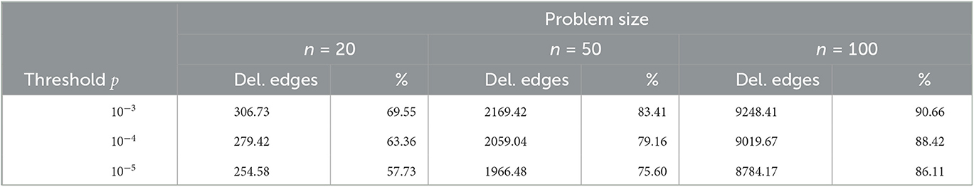
Table 1. Number and percentage of edges deleted for different problem sizes and thresholds (mean over 10,000 instances).
For the GCNDA, these sparse graphs act as a learned problem reduction. Table 2 analyzes the impact of the problem reduction on the size of the instances for the Digital Annealer. For the number of binary variables needed to represent integer variables, for our datasets an upper bound for δ in equation (25) is given as δ = 10. Note however that we can reduce the number of auxiliary binary variables needed by taking into account the upper and lower bound of each integer variable individually before initializing the auxiliary binary variables. As shown in Table 2, the learned problem reduction allows us to reduce the size of our instances, consisting of the QUBO formulation and the inequalities, significantly.
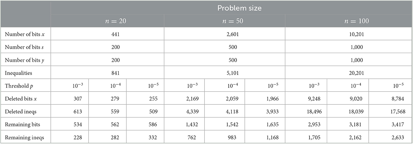
Table 2. Estimation of instance sizes for Digital Annealer after applying learned problem reduction on 10,000 instances.
4.3.2. Experimental results
Tables 3, 4 show the results of our models for the three different problem sizes with beam width b = 1, 000 and b = 10, 000, denoted as 1K and 10K in the model name, for two different datasets and compares our results to results obtained by the previously described exact and heuristic baseline solvers. We report the results for two datasets, the first consists of 1,000 randomly sampled instances from the distribution described in Section 4.2.1. The second dataset is the well-known Solomon benchmark set, which consists of 56 instances with 100 customers. For the smaller problem sizes, we split each instance with 100 customers in two and five instances respectively, with the depot being the same from the original instance. We report the average gap to the groundtruth solution, which was obtained by LKH3, as well as the average calculation time per instance in seconds. As Gurobi was not able to find solutions for all 46 instances of the problem set with n = 50 nodes, the mean cost in Table 5 is not comparable to the other approaches. Even with a time limit of 7,200 s per instance, Gurobi managed to find solutions only for 37 of 46 instances. According to the data presented in Table 4, for instances with n = 20 nodes, Gurobi, an exact solver, exhibited a gap with respect to the best known solutions, although generally not reaching the time limit. This finding can be attributed to Gurobi's inability to identify the globally optimal solutions for all 115 instances of the dataset within the imposed time constraints, despite not reaching the limit for the majority of the cases.
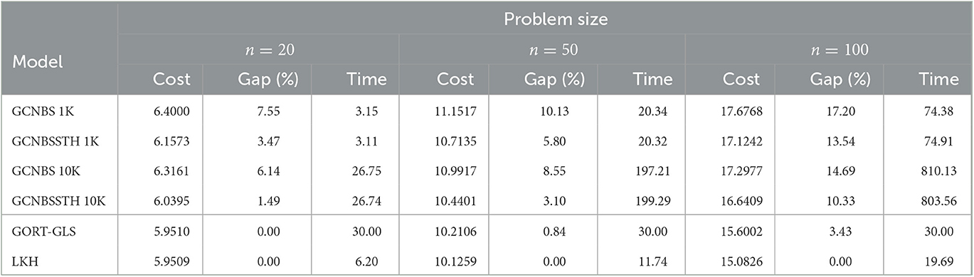
Table 3. Mean cost, gap, and time per instance to solve 1,000 CVRPTW instances.

Table 4. Mean cost, gap, and time per instance to solve the Solomon CVRPTW benchmark set.
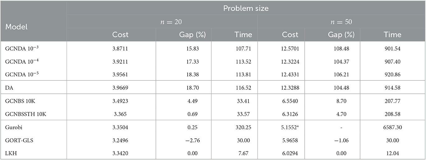
Table 5. Mean cost, gap, and time per instance to solve the Solomon CVRPTW benchmark set R.
In general, our learning-based approach is able to improve its performance over the initial setting by additionally applying the shortest tour heuristic without noticeable implications regarding the computation time. It is evident that both approaches, GCNBS and GCNBSSTH, yield better results for all instance sizes and beam widths for the 1,000 instances dataset in comparison to Solomon's benchmark set [57], which can be attributed to the fact that the neural networks were trained with datasets based on Solomon's benchmark set R [57]. This demonstrates that the performance of the proposed approach is heavily reliant on the selection of training data. In order to achieve generalization within the same problem class, the model must be trained with data that is representative of the underlying distribution, which can vary considerably across different applications. The process of generating suitable training data is a challenging but critical task, as the efficacy of a supervised learning approach is directly influenced by the quality of the data utilized for training.
For small instance sizes, with a beam width of 10,000 GCNBSSTH finds solutions close to the LKH3 results with a mean gap of approximately 1.5% on the dataset used to also train the neural nets and around 2.8% on the Solomon dataset. GCNBS (+STH) outperforms the commercial solver Gurobi [13] in terms of speed for all instance sizes. In fact Gurobi was only able to find solutions for instances with 20 nodes reliably within a time limit of 1,800 s. For instances with 50 nodes, Gurobi was only able to find a valid solution approximately half of the time, whereas for instances with 100 nodes, Gurobi could not find valid solutions within the time limit. Within a setting of similar computation times, the assumption is that similar results regarding solution quality can be expected for instances with 20 nodes by our learning-based approach if trained for the specific dataset distribution. The highly optimized heuristic LKH3 [14] as well as Google's OR-Tools [15] outperformed GCNBSSTH in terms of speed and solution quality on all instance sizes. For smaller instances, Google's OR-Tools perform even better than LKH3, whereas for instances with 100 nodes LKH3 shows the best results. Especially for large instances with 100 nodes the shortcoming of our model becomes apparent, as the beam search becomes computationally expensive for larger instances and beam widths. The computation time mainly depends on the chosen beam width and it seems to be close to a linear correlation between beam width and computation time. Tests have shown that most of the computation time in the current implementation is used in the masking of invalid next nodes with respect to the time windows constraints within the beam search and a more efficient implementation of the masking scheme could lead to significant improvements regarding the computation time.
Table 5 shows the results of our experiments on the Digital Annealer compared to results obtained by GCNBS (+STH) as well as the baseline models. As the amount of time to run experiments on the Digital Annealer was limited, we conducted the experiments on a smaller dataset only consisting of the Solomon benchmark instances from the set R, which was also the baseline distribution for our data generation. The dataset consists of 115 and 46 instances for the problem sizes with 20 and 50 customers, respectively. The asterisk on Gurobi's result for n = 50 indicates that the results are not comparable as for only half of the instances Gurobi was able to find feasible solutions.
The performance of the GCNDA method is inferior to that of GCNBSSTH and especially the baseline models, in terms of both run time and quality of results. The use of integer variables poses a significant challenge for the Digital Annealer (DA) when solving instances of the CVRPTW. As previously mentioned, each integer variable must be represented in binary form, resulting in binary variables for our model, which contains 2n integer variables. As discussed in Section 3.4.4, the requirement to identify the correct assignment of all binary variables introduced for binary expansions poses significant challenges for QUBO and BQP solvers, as it necessitates a considerable number of bit switches. However, the results from Table 5 clearly demonstrate the effectiveness of the learned problem reduction method in improving solution quality by reducing the size of the considered graph for smaller instances. A performance improvement of around 3%, while also accelerating the optimization process, is a promising result. It is reasonable to assume that the decrease in computation time becomes more obvious if a higher time limit is given. As seen in Table 2, the higher the edge probability threshold used in the reduction, the fewer integer variables are required. The risk of the best solutions not being obtained due to the removal of important edges during the reduction process is found to be negligible within the range of solution gaps presented in Table 5. As the size of the CVRPTW problem increases, the optimization of the number of integer variables becomes increasingly challenging. Since the learned problem reduction only applies to the decision variables x, whereas the number of integer variables y and s is not reduced, the effect of the reduction for larger instances is negligible. Given the current version of the DA and the resources available for our experimental study, the limitations of the approach have been reached.
4.3.3. Example solution visualizations
Figures 1, 2 show solution plots for two different instances with 20 nodes as well as the groundtruth tour in the upper left corner and the probabilistic heatmap output of our Graph Convolutional Network in the upper right corner of Figure 1 (left and middle plot in Figure 1, respectively). A darker red color in the heatmap implies a higher probability and only edges with a probability of at least 0.25 are plotted. The gray edges show all edges of the fully connected graph. In Figure 2, one can see the improvement of the solution by applying the shortest tour heuristic. The solution of the beam search in fact uses one vehicle less than the groundtruth tour, but by using one more vehicle, GCNBSSTH is able to lower the total distance traveled and find the best solution. Figure 2 showcases the ability of GCNBSSTH to correctly identify most of the important edges as important, while also excluding most of the irrelevant edges. But in contrast to the solution found in Figure 1, here GCNBSSTH uses one vehicle less than the best solution, illustrating the need for more information regarding other subtours while building the solution in order to find the best solution.
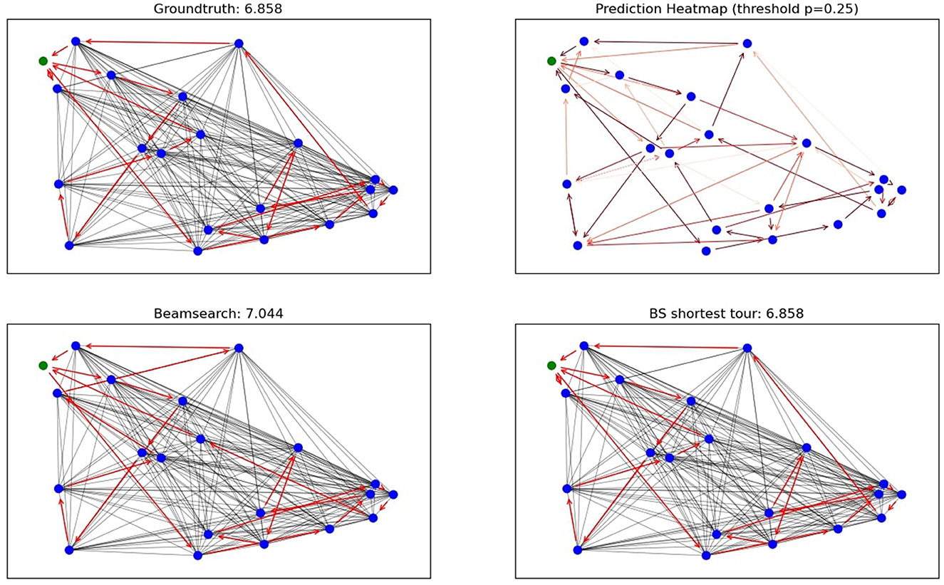
Figure 1. Example solution plot GCNBS and GCNBSSTH for n = 20.
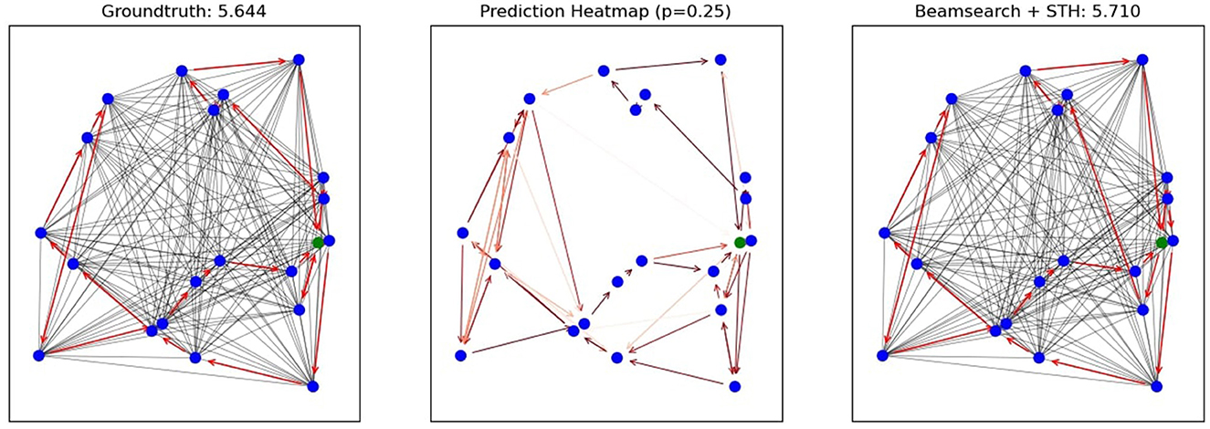
Figure 2. Example solution plot GCNBSSTH for n = 20.
Figure 3 visualizes the optimization process by the Digital Annealer for four different instances. The x-axis refers to the solution time and the two y-axes indicate the energy of the objective function and the constraints (penalties), respectively. The DA starts with a condition where the energy of the objective function is zero and the energy of the penalties is positive. Then the solution is optimized by first decreasing the energy of the penalties to zero, which translates to finding a valid solution, and implies increasing the energy of the objective function. Then, the energy of the objective function is decreased while the energy of the penalties remains at zero.
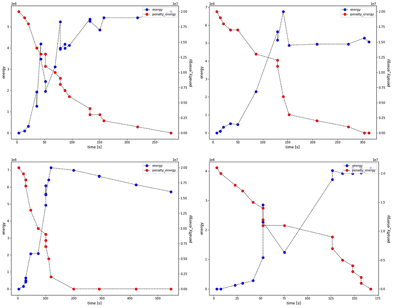
Figure 3. Visualization of the optimization process by the Digital Annealer for four different instances.
5. Discussion
In this paper, we proposed two learning-based approaches to solve the capacitated vehicle routing problem with time windows. The first method combines a Graph Convolutional Network with a classical tree search heuristic, whereas in the second approach the Graph Convolutional Network is used as a learning-based reduction combined with methods from the field of quadratic unconstrained binary optimization in order to solve the problem with quantum-inspired computers.
In conclusion, the proposed approaches for solving the capacitated vehicle routing problem with time windows (CVRPTW) using a Graph Convolutional Network combined with a classical heuristic, a beam search, as well as in combination with quantum-inspired computing methods showed promising results. Although our approach is not as advanced as other existing heuristics and the computational results for the approach using a beam search were not quite as good as those of state-of-the-art highly developed heuristic approaches such as LKH3 [14] and Google's OR-Tools [15], it is still competitive on smaller instances, showing promising results close to the known best results on datasets containing instances with 20 and 50 nodes, respectively, while also outperforming the exact solver Gurobi [13] in terms of solution quality and computation time for larger instances. It is apparent from the computational results that the proposed model is less efficient compared to the highly optimized heuristics that leverage the problem structure through the use of expert knowledge. However, the objective of our approach is to demonstrate the capability of deep learning to construct models capable of solving complex combinatorial optimization problems with minimal dependence on expert knowledge, while simultaneously achieving superior performance compared to existing commercial solvers.
The binary quadratic program (BQP) formulation of the CVRPTW, which we derived from our developed novel quadratic unconstrained binary optimization (QUBO) formulation of the CVRPTW, was solved on Fujitsu's Digital Annealer by applying a deep neural network as a learned problem reduction . This demonstrates the potential of using learned problem reductions in improving solution quality and reducing computation time on quantum(-inspired) computers. However, the large size of CVRPTW instances and the requirement for a significant number of integer variables to model the problem as a quadratic unconstrained binary optimization problem make it challenging to optimize for larger instances, even with the reduction of the instance size. Further research is necessary to identify more efficient problem representations to effectively solve CVRPTW via QUBO and to handle integer variables in a more efficient way. The computational experiments conducted have highlighted a significant dependency of the proposed approach on the training data used, as evidenced by the inferior performance observed for a data set exhibiting a slightly different data distribution when compared to instances sharing the same data distribution.
Our approaches represent novel and innovative learning-based solutions for the CVRPTW and offer an alternative solution that may be suitable for certain applications. Further research is needed to improve the performance and to validate its results on a larger and more diverse set of inputs. To further develop approaches that use deep neural networks build solutions constructively is a promising direction for future research, as the constructive nature allows for efficient handling of hard constraints, such as time windows, which can be difficult for both neural combinatorial optimization and local search heuristics to effectively address. These types of constraints are particularly challenging in these methods due to the need to maintain feasibility while adapting a solution. The use of deep learning in this context represents a promising direction for future work in solving the capacitated vehicle routing problem with hard constraints, but further research is necessary to develop more sophisticated methods for constructing solutions. Moving forward, our research aims to overcome the limitations of the beam search algorithm by incorporating contextual information from partially constructed solutions to guide the selection of the next node, and integrating a deep neural network in an autoregressive manner. Our objective is to enhance the efficiency and accuracy of the search process for complex problems by leveraging these advanced techniques.
Combining classical approaches with deep learning has the potential to improve solution methods for a wide range of combinatorial optimization problems, as it is not necessary to have in-depth, specific knowledge about the structures of the problem and its solution space in order to develop approaches that can provide usable solutions that are faster and better than available commercial solvers.
Data availability statement
The raw data supporting the conclusions of this article will be made available by the authors, without undue reservation.
Author contributions
JD confirms sole responsibility for model conception and design, data generation, computational experiments, analysis and interpretation of results, and manuscript preparation.
Funding
Open Access funded by the Deutsche Forschungsgemeinschaft (DFG, German Research Foundation) Projektnummer 491268466 and the Hamburg University of Technology (TUHH) in the funding programme Open Access Publishing.
Acknowledgments
We would like to express our gratitude to the team at Fujitsu Technology Solutions, particularly Markus Kirsch, for their valuable collaboration and assistance in utilizing Fujitsu's Digital Annealer.
Conflict of interest
The author declares that the research was conducted in the absence of any commercial or financial relationships that could be construed as a potential conflict of interest.
Publisher's note
All claims expressed in this article are solely those of the authors and do not necessarily represent those of their affiliated organizations, or those of the publisher, the editors and the reviewers. Any product that may be evaluated in this article, or claim that may be made by its manufacturer, is not guaranteed or endorsed by the publisher.
References
1. Toth P, Vigo D, editors. Vehicle Routing. Philadelphia, PA: Society for Industrial and Applied Mathematics (2014).
2. Desaulniers G, Lessard F, Hadjar A. Tabu search, partial elementarity, and generalized k-path inequalities for the vehicle routing problem with time windows. Transport Sci. (2008) 42:387–404. doi: 10.1287/trsc.1070.0223
3. Prescott-Gagnon E, Desaulniers G, Rousseau LM. A branch-and-price-based large neighborhood search algorithm for the vehicle routing problem with time windows. Networks. (2009) 54:190–204. doi: 10.1002/net.20332
4. Shaw P. Using constraint programming and local search methods to solve vehicle routing problems. In: Principles and Practice of Constraint Programming – CP98. Berlin, Heidelberg (1998). p. 417–31.
5. Chen X, Tian Y. Learning to perform local rewriting for combinatorial optimization. In: Proceedings of the 33rd International Conference on Neural Information Processing Systems. Vancouver, BC: Curran Associates Inc. (2019). p. 6281–92.
6. Lu H, Zhang X, Yang S. A learning-based iterative method for solving vehicle routing problems. In: 8th International Conference on Learning Representations, 2020 (2020).
7. Nazari M, Oroojlooy A, Snyder LV, Takác M. Reinforcement Learning for Solving the Vehicle Routing Problem. In:Bengio S, Wallach H, Larochelle H, Grauman K, Cesa-Bianchi N, , editors. Proceedings of the 32nd International Conference on Neural Information Processing Systems, NIPS'18. Montréal, QC: Curran Associates Inc. (2018). p. 9861–71.
8. Kool W, van Hoof H, Welling M. Attention, learn to solve routing problems! In: 7th International Conference on Learning Representations, 2019 (New Orleans, LA). (2019).
9. Falkner JK, Schmidt-Thieme L. Learning to solve vehicle routing problems with time windows through joint attention. arXiv preprint arXiv:2006.09100 (2020). doi: 10.48550/arXiv.2006.09100
10. Savelsbergh MWP. Local search in routing problems with time windows. Ann Operat Res. (1985) 4:285–305.
11. Joshi CK, Laurent T, Bresson X. An efficient graph convolutional network technique for the travelling salesman problem. arXiv preprint arXiv:1906.01227 (2019). doi: 10.48550/arXiv.1906.01227
12. Sun Y, Ernst A, Li X, Weiner J. Generalization of machine learning for problem reduction: a case study on travelling salesman problems. OR Spectrum. (2020) 43:607–33. doi: 10.1007/s00291-020-00604-x
13. Gurobi Optimization, LLC,. Gurobi Optimizer Reference Manual. (2022). Available online at: https://www.gurobi.com
14. Helsgaun K. An Extension of the Lin-Kernighan-Helsgaun TSP Solver for Constrained Traveling Salesman and Vehicle Routing Problems. Technical report. Roskilde Universitet, Roskilde (2017).
15. Perron L, Furnon V. Google OR-Tools (2022). Available online at: https://developers.google.com/optimization/
16. Vinyals O, Fortunato M, Jaitly N. Pointer networks. In:Cortes C, Lawrence N, Lee D, Sugiyama M, Garnett R, , editors. Advances in Neural Information Processing Systems. vol. 28. Montréal, QC: Curran Associates, Inc. (2015). p. 2692–700.
17. Bello I, Pham H, Le QV, Norouzi M, Bengio S. Neural combinatorial optimization with reinforcement learning. arXiv preprint arXiv:1611.09940 (2016). doi: 10.48550/arXiv.1611.09940
18. Rumelhart DE, Hinton GE, Williams RJ. Learning internal representations by error propagation. In:Rumelhart DE, McClelland JL, , editors. Parallel Distributed Processing: Explorations in the Microstructure of Cognition, Volume 1: Foundations. Cambridge, MA: MIT Press (1986). p. 318–62.
19. Joshi CK, Laurent T, Bresson X. On learning paradigms for the travelling salesman problem. arXiv preprint arXiv:1910.07210 (2019). doi: 10.48550/arXiv.1910.07210
20. Kwon YD, Choo J, Kim B, Yoon I, Gwon Y, Min S. POMO: policy optimization with multiple optima for reinforcement learning. In:Larochelle H, Ranzato M, Hadsell R, Balcan MF, Lin H, , editors. Advances in Neural Information Processing Systems. vol. 33. Curran Associates, Inc. (2020). p. 21188–98.
21. Kaempfer Y, Wolf L. Learning the multiple traveling salesmen problem with permutation invariant pooling networks. arXiv preprint arXiv:1803.09621 (2018). doi: 10.48550/arXiv.1803.09621
22. Delarue A, Anderson R, Tjandraatmadja C. Reinforcement learning with combinatorial actions: an application to vehicle routing. In:Larochelle H, Ranzato M, Hadsell R, Balcan MF, Lin H, , editors. Proceedings of the 34th International Conference on Neural Information Processing Systems. Curran Associates, Inc. (2020). p. 609–20.
23. Peng B, Wang J, Zhang Z. A deep reinforcement learning algorithm using dynamic attention model for vehicle routing problems. In:Li K, Li W, Wang H, Liu Y, , editors. Artificial Intelligence Algorithms and Applications. Singapore: Springer (2020). p. 636–50.
24. Bengio Y, Lodi A, Prouvost A. Machine learning for combinatorial optimization: A methodological tour d'horizon. Eur J Oper Res. (2021) 290:405–21. doi: 10.1016/j.ejor.2020.07.063
25. Medress MF, Cooper FS, Forgie JW, Green C, O'Malley DHKMH, Neuburg EP, et al. Speech understandingsystems: report of a steering committee. Artif Intell. (1977) 9:307–16.
26. Nowak A, Villar S, Bandeira AS, Bruna J. Revised note on learning algorithms for quadratic assignment with graph neural networks. arXiv preprint arXiv:1706.07450 (2017). doi: 10.48550/arXiv.1706.07450
27. Scarselli F, Gori M, Tsoi AC, Hagenbuchner M, Monfardini G. The graph neural network model. IEEE Trans Neural Netw. (2009) 20:61–80. doi: 10.1109/TNN.2008.2005605
28. Bresson X, Laurent T. Residual gated graph ConvNets. arXiv preprint arXiv:1711.07553 (2017). doi: 10.48550/arXiv.1711.07553
29. Falkner JK, Thyssens D, Schmidt-Thieme L. Large neighborhood search based on neural construction heuristics. arXiv preprint arXiv:2205.00772 (2022). doi: 10.48550/arXiv.2205.00772
30. Wang Y, Sun S, Li W. Hierarchical reinforcement learning for vehicle routing problems with time windows. In: Proceedings of the Canadian Conference on Artificial Intelligence (2021).
31. Gao L, Chen M, Chen Q, Luo G, Zhu N, Liu Z. Learn to design the heuristics for vehicle routing problem. arXiv preprint arXiv:2002.08539 (2020).
32. Veličković P, Cucurull G, Casanova A, Romero A, Licš P, Bengio Y. Graph attention networks. In: 6th International Conference on Learning Representations, ICLR 2018 (Vancouver, BC). (2018).
33. Silva MAL, de Souza SR, Freitas Souza MJ, Bazzan ALC. A reinforcement learning-based multi-agent framework applied for solving routing and scheduling problems. Expert Syst Appl. (2019) 131:148–71. doi: 10.1016/j.eswa.2019.04.056
34. Irnich S, Desaulniers G. Shortest path problems with resource constraints. In:Desaulniers G, Desrosiers J, Solomon MM, , editors. Column Generation. Boston, MA: Springer (2005) p. 33–65.
35. Dror M. Note on the complexity of the shortest path models for column generation in VRPTW. Operat Res. (1994) 42:977–8.
36. Kohl N, Desrosiers J, Madsen OBG, Solomon MM, Soumis F. 2-path cuts for the vehicle routing problem with time windows. Transport Sci. (1999) 33:101–16.
37. Jepsen M, Petersen B, Spoorendonk S, Pisinger D. Subset-row inequalities applied to the vehicle-routing problem with time windows. Operat Res. (2008) 56:497–511. doi: 10.1287/opre.1070.0449
38. Pecin D, Pessoa A, Poggi M, Uchoa E. Improved branch-cut-and-price for capacitated vehicle routing. In:Lee J, Vygen J, , editors. Integer Programming and Combinatorial Optimization. Bonn: Springer Cham (2014). p. 393–403.
39. Pecin D, Contardo C, Desaulniers G, Uchoa E. New enhancements for the exact solution of the vehicle routing problem with time windows. INFORMS J Comput. (2017) 29:489–502. doi: 10.1287/ijoc.2016.0744
40. Feillet D, Dejax P, Gendreau M, Gueguen C. An exact algorithm for the elementary shortest path problem with resource constraints: application to some vehicle routing problems. Networks. (2004) 44:216–29. doi: 10.1002/net.20033
41. Boland N, Dethridge J, Dumitrescu I. Accelerated label setting algorithms for the elementary resource constrained shortest path problem. Operat Res Lett. (2006) 34:58–68. doi: 10.1016/j.orl.2004.11.011
42. Feillet D, Gendreau M, Rousseau LM. New refinements for the solution of vehicle routing problems with branch and price. Inform Syst Operat Res. (2007) 45:239–56. doi: 10.3138/infor.45.4.239
43. Baldacci R, Mingozzi A, Roberti R. New route relaxation and pricing strategies for the vehicle routing problem. Operat Res. (2011) 59:1269–83. doi: 10.1287/opre.1110.0975
44. Baldacci R, Mingozzi A, Roberti R. Recent exact algorithms for solving the vehicle routing problem under capacity and time window constraints. Eur J Operat Res. (2012) 218:1–6. doi: 10.1016/j.ejor.2011.07.037
45. Papalitsas C, Andronikos T, Giannakis K, Theocharopoulou G, Fanarioti S. A QUBO model for the traveling salesman problem with time windows. Algorithms. (2019) 12:224. doi: 10.3390/a12110224
46. Salehi O, Glos A, Miszczak JA. Unconstrained binary models of the travelling salesman problem variants for quantum optimization. Quant Inform Process. (2022) 21, 67. doi: 10.1007/s11128-021-03405-5
47. Suen WY, Parizy M, Lau HC. Enhancing a QUBO solver via data driven multi-start and its application to vehicle routing problem. In: Proceedings of the Genetic and Evolutionary Computation Conference Companion. Boston, MA: ACM (2022). p. 2251–7.
48. Akeb H, Bouchakhchoukha A, Hifi M. A beam search based algorithm for the capacitated vehicle routing problem with time windows. In: Federated Conference on Computer Science and Information Systems 2013 (Kraków). (2013). p. 329–36.
49. Kool W, van Hoof H, Gromicho J, Welling M. Deep policy dynamic programming for vehicle routing problems. In:Pierre Schaus, , editor. Integration of Constraint Programming, Artificial Intelligence, and Operations Research. Los Angeles, CA: Springer International Publishing (2022). p. 190–213.
50. Ioffe S, Szegedy C. Batch normalization: accelerating deep network training by reducing internal covariate shift. In: Proceedings of the 32nd International Conference on International Conference on Machine Learning (Lille). (2015). p. 448–56.
51. Glover FW, Kochenberger GA, Du Y. Quantum Bridge Analytics I: a tutorial on formulating and using QUBO models. arXiv preprint arXiv:1811.11538 (2018). doi: 10.48550/arXiv.1811.11538
52. Kallehauge B, Larsen J, Madsen OBG, Solomon MM. Vehicle routing problem with time windows. In:Desaulniers G, Desrosiers J, Solomon MM, , editors. Column Generation. Boston, MA: Springer US (2005). p. 67–98.
53. Fujitsu. Digital Annealer (2022). Available online at: http://www.fujitsu.com/global/digitalannealer/
54. Vyskočil T, Pakin S, Djidjev HN. Embedding inequality constraints for quantum annealing optimization. In:Feld S, Linnhoff-Popien C, , editors. Quantum Technology and Optimization Problems. Cham: Springer International Publishing (2019). p. 11–22.
55. Sao M, Watanabe H, Musha Y, Utsunomiya A. Application of digital annealer for faster combinatorial optimization. Fujitsu Sci Tech J. (2019) 55:45–51.
56. Paszke A, Gross S, Chintala S, Chanan G, Yang E, DeVito Z, et al. Automatic differentiation in PyTorch. In: NIPS-W (Long Beach, CA). (2017).
57. Solomon MM. Algorithms for the vehicle routing and scheduling problems with time window constraints. Operat Res. (1987) 35:254–65. doi: 10.1287/opre.35.2.254
Keywords: deep learning, graph convolutional network, beam search, vehicle routing, time windows, quadratic unconstrained binary optimization
Citation: Dornemann J (2023) Solving the capacitated vehicle routing problem with time windows via graph convolutional network assisted tree search and quantum-inspired computing. Front. Appl. Math. Stat. 9:1155356. doi: 10.3389/fams.2023.1155356
Received: 31 January 2023; Accepted: 08 June 2023;
Published: 22 June 2023.
Edited by:
Andreas M. Tillmann, Technical University of Braunschweig, GermanyReviewed by:
Alberto Ochoa Zezzatti, Universidad Autónoma de Ciudad Juárez, MexicoJosé Alberto Hernández-Aguilar, Autonomous University of the State of Morelos, Mexico
Sebastian Stiller, Technical University of Braunschweig, Germany
Tim Niemann, Technical University of Braunschweig, Germany, in collaboration with reviewer SS
Copyright © 2023 Dornemann. This is an open-access article distributed under the terms of the Creative Commons Attribution License (CC BY). The use, distribution or reproduction in other forums is permitted, provided the original author(s) and the copyright owner(s) are credited and that the original publication in this journal is cited, in accordance with accepted academic practice. No use, distribution or reproduction is permitted which does not comply with these terms.
*Correspondence: Jorin Dornemann, am9yaW4uZG9ybmVtYW5uQHR1aGguZGU=