On composite length-biased exponential-Pareto distribution: Properties, simulation, and application in actuarial science

The composite length-biased exponential-Pareto (CLBEP) distribution is a new composite distribution that is introduced in this article. This model's probability density function, moments, and quantiles, among other statistical characteristics, are determined mathematically. The parameters' maximum-likelihood estimation and stochastic ordering are discussed. A comparison study with other new composite and conventional distributions is also included. Specifically, using two actual fire insurance data sets, the goodness of fit of this new model is contrasted with the composite exponential-Pareto, composite lognormal-Pareto, and composite Rayleigh-Pareto distributions (Algerian and Danish fire insurance losses).

2010 AMS subject classifications: 62E10; 60E05.

1. Introduction

Currently, digital methods are being used in the fields of biology, economics, physical sciences, statistical sciences, and other fields. In the applications of other fields as well as in daily life, the statistical sciences are essential. Probability distributions are frequently the foundation of statistical science because many problems in these fields frequently do not follow one of the fundamental probability distributions. Actuarial science and finance generally use common distributions to express their data on payments, quantity and number of claims, and premium computation. Examples of these distributions are exponential, Poisson, length-biased exponential, and Pareto.

The length-biased exponential distribution, on the other hand, offers a wide range of practical applications in several industries (reliability, actuarial science, survival analysis, and mathematical financiers). The lifetime of a phenomenon with no memory, no aging, no wear and tear, or the profits of an insurance company, or various models of surpluses and financial assets, are frequently modeled using the length-biased exponential distribution.

The modeling of unimodal insurance loss data with a long tail appeals to actuaries. Distributions that may replicate the heavy tail of insurance loss data are necessary to provide a sufficiently precise estimate of the degree of connected business risk, including gamma, Pareto, length-biased exponential, Rayleigh lognormal, and Weibull.

For example, if there are both modest and significant losses, insurance companies may experience losses. When modeling very large losses, practitioners seem to favor the Pareto distribution for size distribution. Length-biased exponential, lognormal, Rayleigh, or Weibull models are preferred when the losses are composed of smaller values with high frequencies and larger losses with low frequencies [1]. Nevertheless, no conventional size model can simultaneously account for losses that are both minor and significant. Unlike length-biased, lognormal, Rayleigh, or Weibull exponential models, which have a positive general fit but fit the tail poorly, Pareto models actually fit the tail well.

When modeling data that have heavy tails, the composite distributions appear appropriate. For instance, the one-parameter exponential-Pareto (exp-Pareto) model and the one-parameter inverse gamma-Pareto (IG-Pareto) model have both been proposed as potential models for the modeling of insurance data. When they are fitted to well-known insurance data sets, such as the Danish fire insurance data set, they still are unable to perform satisfactorily. So, the model needs to be improved. By exponentiation of the random variable linked to the probability density function (pdf) of an inverse gamma-Pareto distribution, Liu and Ananda [2] suggested an improved version of the one-parameter IG-Pareto model. Their suggested model outperformed the original model significantly across several data sets. Furthermore, there are other composite models such as the composite lognormal-Pareto (cLP) model (see Scollnik [3] and composite Rayleigh-Pareto (cRP) model (see Benatmane et al. [4]). For more details see [5–12].

As a result, we suggest, in this study, a novel composite distribution that blends length-biased and Pareto exponential distributions. This effort aims to introduce a new composite distribution. As a result, the CLBEP distribution has a single parameter. It is simple to determine mathematical qualities in an explicit form. Due to its composition (two types of distributions that can be simulated for survival analysis and actuarial purposes), this new distribution offers advantages. Many real-life data sets can be analyzed using the CLBEP model, which provides suitable fits to these data sets.

The current article is structured as follows: The composite length-biased exponential-Pareto distribution and some of its statistical characteristics are discussed in Section 2. The estimation of parameters is addressed in Section 3. A numerical example with a comparison of various classical and composite models using two real data sets is provided in Section 4.

2. Formulation of the CLBEP distribution

For many theoretical issues, the length-biased exponential and Pareto distributions might not be adequate. We created the composite length-biased exponential-Pareto (CLBEP) distribution, based on the composite transformation, to have a flexible model. Let T be an arbitrary random variable with density function

$f(t;\theta )=\{\begin{array}{cc}c{f}_1(t)& 0<t\le \theta \\ c{f}_2(t)& \theta \le t<\infty \end{array}$

where f₁ is a length-biased exponential density, f₂ is a two-parameter Pareto density, and c is the normalizing constant. Hence,

$\begin{array}{c}\hfill f_1(t)=\frac{t}{{\lambda }^2}\exp \left(-\frac{t}{\lambda }\right),0<t\le \infty ,\hfill \\ \hfill f_2(t)=\frac{\alpha {\theta }^{\alpha }}{t^{\alpha +1}},t>\theta ,\hfill \end{array}$

where λ, α, and θ are unknown non-negative parameters. To obtain a composite smooth density function, we use the continuity and differentiability conditions at the threshold point θ, i.e.,

$\{\begin{array}{c}{f}_1(\theta )=f_2(\theta )\\ \frac{d}{dt}{f}_1(\theta )=\frac{d}{dt}{f}_2(\theta ).\end{array}$

These two restrictions give

$\{\begin{array}{c}\frac{\theta }{{\lambda }^2}\exp \left(-\frac{\theta }{\lambda }\right)=\frac{\alpha }{\theta }\\ \frac{\left(\lambda -\theta \right)}{{\lambda }^3}\exp (-\frac{\theta }{\lambda })=\frac{-\alpha \left(\alpha +1\right)}{{\theta }^2}.\end{array}$

After some calculation, we get

$\{\begin{array}{c}2-\beta +\left({\beta }^2\exp (-\beta )\right)=0\\ \alpha ={\beta }^2\exp (-\beta )\end{array}\text{with }\beta =\frac{\theta }{\lambda }.$

Using the numerical methods, we find

$\{\begin{array}{c}\beta =2.5118\\ \alpha =0.51181.\end{array}$

To find the normalizing constant, we use the density condition $({\displaystyle \underset{0}{\overset{\infty }{\int }}}f(t,\theta )dt=1),$ which has

$\begin{array}{l}c=\frac{1}{e^{-\frac{\theta }{\lambda }}\left(\frac{\theta }{\lambda }+1\right)+2}\\ =\frac{1}{e^{-\beta }\left(\beta +1\right)+2}=0.43766.\end{array}$

Since f(t; θ) can be expressed as

$\begin{array}{ll}f(t;\theta )=\{\begin{array}{cc}\frac{2.7613t}{{\theta }^2}\exp \left(\frac{-2.5118t}{\theta }\right)& 0<t\le \theta \\ \frac{0.224}{t^{1.51181}}{\theta }^{0.51181}& \theta \le t<\infty .\end{array}& (1)\end{array}$

2.1. Statistical properties of the CLBEP distribution

In this subsection, many statistical properties are presented, such as the behavior of PDF and quantile function, as well as the moments and stochastic ordering.

$\underset{t\to 0}{\lim }f(t;\theta )=0\text{ and }\underset{t\to \infty }{\lim }f(t;\theta )=0.$

The following proposition states that there is one shape for the PDF of the CLBEP distribution. Furthermore, the plots of PDF for some parameter value of the proposed model are presented in Figure 1.

FIGURE 1

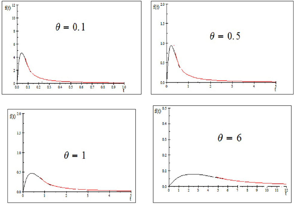
Figure 1. The plots of PDF for some parameter value of θ.

Proposition 1. The PDF f(t; θ) in Equation (1) of the CLBEP distribution is unimodal for θ > 0.

Proof. The first derivative of f(t; θ) is

$\begin{array}{l}\frac{df(t;\theta )}{dt}\\ =\{\begin{array}{cc}-\frac{0.0002}{{\theta }^3}\exp \left(-2.5118\frac{t}{\theta }\right)\left(34679t-13807\theta \right)& 0<t\le \theta \\ -\frac{0.33865}{t^{2.5118}}{\theta }^{0.51181}& \theta \le t<\infty .\end{array}\end{array}$

The CLBEP distribution is unimodal with maximum value at the point $\widehat{t}=0.39814\theta ,$ where the unique mode is t_mod = 0.39814θ.

2.2. Cumulative distribution function and moments of the CLBEP distribution

The cumulative distribution function (c.d.f.) of this composite model is

$\begin{array}{ll}F(t;\theta )=\{\begin{array}{cc}0.43768\left(1-(1+\frac{2.5118t}{\theta })\exp \left(\frac{-2.5118t}{\theta }\right)\right)& 0<t\le \theta \\ 1-0.43768{\left(\frac{\theta }{t}\right)}^{0.51181}& \theta \le t<\infty \end{array}& (2)\end{array}$

The kth moment about the origin of the CLBEP distribution can be obtained as:

$\begin{array}{l}E\left(T^k\right)=-\frac{0.43768{\theta }^k}{{\left(2.5118\right)}^k}\left(\Gamma \left(k+2,2.5118\right)-\Gamma \left(k+2\right)\right)\\ +{0.224{\theta }^{0.51181}\left(\frac{x^{k-1.5118}}{k-1.5118}\right)|}_{\theta }^{\infty },\end{array}$

which E(T^k) = ∞ (infinite), for k ≥ 2.

The mean of the CLBEP distribution is given by

$E\left(T\right)=0.16003\theta +0.43767.$

2.3. The quantile function of the CLBEP distribution

The quantile function of the CLBEP distribution is given in the following theorem.

Theorem 1. The quantile function of the CLBEP distribution is

$F_T^{-1}\left(u\right)=\{\begin{array}{c}\frac{-\theta }{2.5118}-\frac{\theta }{2.5118}{W}_{-1}(\frac{u}{0.43768e}-e^{-1})\text{ if 0}<u<u_0\\ \theta {\left(\frac{0.43768}{\left(1-u\right)}\right)}^{1.9539}\text{ if }{u}_0<u<\text{1}\end{array}$

where u₀ = 0.43768.

Proof. For u ∈ ]0;u₀[, we have to solve the equation F(t) = u with respect to t, t > 0

$\begin{array}{l}0.43768\left(1-(1+\frac{2.5118t}{\theta })\exp \left(\frac{-2.5118t}{\theta }\right)\right)=u\\ -(1+\frac{2.5118t}{\theta })\exp \left(\frac{-2.5118t}{\theta }\right)=\frac{u}{0.43768}-1\end{array}$

Multiplying by e⁻¹ both sides, we find

$\begin{array}{l}-(1+\frac{2.5118t}{\theta })\exp \left(\frac{-2.5118t}{\theta }\right)e^{-1}=(\frac{u}{0.43768}-1)e^{-1}\\ W(z)exp(W(z))=z\end{array}$

We see that $-(1+\frac{2.5118t}{\theta })$ is the Lambert W function of the real argument $(\frac{u}{0.43768}-1)e^{-1}.$ Then, we have

$\begin{array}{ll}W(\frac{u}{0.43768e}-e^{-1})=-1-\frac{2.5118t}{\theta }.& (3)\end{array}$

Moreover, for any θ, t > 0, it is immediate that $-(1+\frac{2.5118t}{\theta })<0,$ and it can also be checked that

$(\frac{u}{0.43768e}-e^{-1})\in \left]\frac{-1}{e};0\right[$ since u ∈ ]0;u₀[

Therefore, by taking into account the properties of the negative branch of the Lambert W function, Equation (3) becomes

$W_{-1}(\frac{u}{0.43768e}-e^{-1})=-(1+\frac{2.5118t}{\theta }).$

Finally, ∀θ > 0, $t=F_T^{-1}(u),$

$F_T^{-1}\left(u\right)=\frac{-\theta }{2.5118}-\frac{\theta }{2.5118}{W}_{-1}(\frac{u}{0.43768e}-e^{-1}),\text{where }0<u<u_0.$

Now, for u ∈ ]u₀; 1[, we have to solve the equation F(t) = u with respect to t, t > 0

$1-0.43768{\left(\frac{\theta }{t}\right)}^{0.51181}=u$

it is easy to find

$F_T^{-1}\left(u\right)=\theta {\left(\frac{0.43768}{\left(1-u\right)}\right)}^{1.9539}\text{ where }{u}_0<u<1.$

2.4. Stochastic ordering

Consider two random variables Z₁ and Z₂. Then, Z₁ is said to be smaller than Z₂ in the following cases:

1. Stochastic order (Z₁ <_S Z₂ ), if F_Z1(t) < F_Z2(t), ∀t.

2. Convex order (Z₁ ≤_cx X₂), if for all convex functions Ψ and provided expectation exists, E[Ψ(Z₁)] ≤ E[Ψ(Z₂)].

3. Hazard rate order (Z₁ ≤_hr Z₂), if h_Z1(t) ≥ h_Z2(t), ∀t.

4. Likelihood ratio order (Z₁ <_lr Z₂), if $\frac{f_{Z_1}(t)}{f_{Z_2}(t)}$ is decreasing in t.

Remark 1. Likelihood ratio order ⇒ hazard rate order ⇒ stochastic order, If E[Z₁] = E[Z₂], then convex order ⇔ stochastic order.

Theorem 2. Let Z_i ∽ CLBEP distribution (θ_i); i = 1, 2 be two random variables. If θ₁ ≤ θ₂, then Z₁ <_lr Z₂, Z₁ <_hr Z₂; Z₁ <_S Z₂ and Z₁ ≤_cx Z₂.

Proof.

Case I: 0 < t ≤ θ

We have

$\frac{f_{Z_1}(t;{\theta }_1)}{f_{Z_2}\left(t;{\theta }_2\right)}=\frac{{\theta }_2^2}{{\theta }_1^2}\exp \left(\frac{-2.5118t}{{\theta }_1}+\frac{2.5118t}{{\theta }_2}\right).$

Using the $ln\left(\frac{f_{Z_1}(t;{\theta }_1)}{f_{Z_2}(t;{\theta }_2)}\right)$ for simplification, we can find

$\frac{d}{dt}\ln \left(\frac{f_{Z_1}(t;{\theta }_1)}{f_{Z_2}\left(t;{\theta }_2\right)}\right)=\frac{2.5118{\theta }_2^2}{{\theta }_1^2}\left(\frac{{\theta }_1-{\theta }_2}{{\theta }_1{\theta }_2}\right).$

To this end, if θ₁ ≤ θ₂, we have $\frac{d}{dt}ln\left(\frac{f_{Z_1}(t;{\theta }_1)}{f_{Z_2}(t;{\theta }_2)}\right)\le 0$. This means that Z₁ <_lr Z₂.

Case II: θ ≤ t < ∞

We have

$f_{Z_1}(t;{\theta }_1)-f_{Z_2}\left(t;{\theta }_2\right)=\frac{0.26148}{t^{1.51181}}\left({\theta }_1^{0.51181}-{\theta }_2^{0.51181}\right).$

We can see, if θ₁ ≤ θ₂, then f_Z2(t; θ₂) ≤ f_Z2(t; θ₂). Furthermore, according to Remark 1, the theorem is proved.

3. Generating random values from the CLBEP distribution

3.1. Parameter estimation

In this section, we will introduce two methods of estimating the unknown parameter θ.

3.1.1. An ad hoc procedure based on percentiles

The following ad hoc procedure provides a closed form for the parameter θ, estimated using percentiles. Let t₁, t₂, …, t_n be a random sample from the CLBEP model. Assume that t₁ ≤ t₂ ≤… ≤ t_n and t_m ≤ θ ≤ t_m+1. Based on percentiles, the parameter θ can be estimated, as the pth percentile, where p = F(θ)

$p=0.43768\left(1-(1+\frac{2.5118\theta }{\theta })\exp \left(\frac{-2.5118\theta }{\theta }\right)\right)=0.31299.$

According to Klugman et al. [1], we have a smooth empirical estimate of the pth percentile given by

$\widehat{\theta }=(1-h)t_m+h{t}_{m+1}$

with

$\begin{array}{ll}\{\begin{array}{c}m=[(n+1)p]\\ h=(n+1)p-m.\end{array}& (4)\end{array}$

The Pareto distribution or the length-biased exponential distribution will be a more superior model than the composite length-biased exponential-Pareto distribution according as $\widehat{\theta }$ is closer to t₁ or t_n.

3.1.2. Maximum-likelihood estimation

Assume again that t₁ ≤ t₂ ≤… ≤ t_n and t_m ≤ θ ≤ t_m+1. Then, the likelihood function is

$\begin{array}{l}L(t_1,\mathrm{\dots },t_n;\theta )={\displaystyle \prod _{i=1}^{n}f}(t_i)={\displaystyle \prod _{i=1}^m{f}_1}(t_i){\displaystyle \prod _{i=m+1}^n{f}_2}(t_i)\\ ={\displaystyle \prod _{i=1}^{m}2}.7613\frac{t_i}{{\theta }^2}\exp \left(-2.51181\frac{t_i}{\theta }\right){\displaystyle \prod _{i=m+1}^n\frac{\left(0.224\right)}{t_{i.}^{1.51181}}}{\theta }^{0.51181}\\ ={\left(2.7613\right)}^m{\left(0.224\right)}^{n-m}{\theta }^{0.51181\left(n-m\right)-2m}{e}^{\frac{-2.51181}{\theta }{\displaystyle {\sum }_{i=1}^m{t}_i}}\\ \frac{{\displaystyle \prod _{i=1}^m{t}_i}}{{\displaystyle \prod _{i=m+1}^n{t}_i^{1.51181}}}\\ =k{\theta }^{0.51181n-2.51181m}{e}^{\left(\frac{-2.51181}{\theta }{\displaystyle {\sum }_{i=1}^m{t}_i}\right)}.\end{array}$

with

$k={\left(2.7613\right)}^m{\left(0.224\right)}^{n-m}\frac{{\displaystyle \prod _{i=1}^m{t}_i}}{{\displaystyle \prod _{i=m+1}^n{t}_i^{1.51181}}}.$

Define $lnL=lnk+(0.51181n-2.51181m)ln\theta +\left(\frac{-2.51181}{\theta }\sum _{i=1}^m{t}_i\right)$.

Differentiating ln L with respect to θ gives

$\frac{d\ln L}{d\theta }=\frac{0.51181n-2.51181m}{\theta }+\frac{2.51181{\displaystyle {\sum }_{i=1}^m{t}_i}}{{\theta }^2}.$

Hence, the solution of the likelihood equation $\frac{dlnL}{d\theta }=0$ is

$\begin{array}{ll}\widehat{\theta }=\frac{2.51181m{\overline{t}}_m}{2.251181m-0.51181n},\text{ if }\frac{n}{m}\ne 4.9\text{ and }{\overline{t}}_m=\frac{{\displaystyle {\sum }_{i=1}^m{t}_i}}{m}.& (5)\end{array}$

Since this estimator requires the value of m, we recommend the following algorithm (see Teodorescu and Vernic [13]):

4. Numerical and application examples

In this section, the estimation procedure described in Section 3 has been explained using two data samples generated from the CLBEP model. The generating algorithm used is based on the inversion of the c.d.f. (Equation 2).

4.1. Example

The data set given in this subsection, consisting of 108 values, was sampled from a length-biased exponential-Pareto population with parameter θ = 5 (see Table 1 in the Appendix).

The estimated values of the parameter are:

- By Algorithm 1, m = 39: ${\widehat{\theta }}_1=5.0536.$

- By Algorithm 2, MLE Step 1: ${\widehat{\theta }}_2=4.9812.$

- By Algorithm 2, MLE Step 2 : ${\widehat{\theta }}_3=4.9810.$

ALGORITHM 1

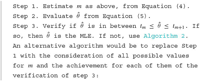
Algorithm 1. Estimate θ using MLE.

ALGORITHM 2

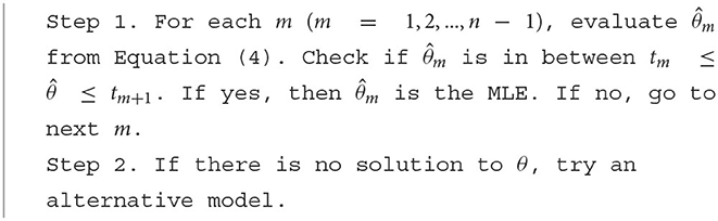
Algorithm 2. Estimate θ using percentiles.

We notice that Algorithm 2 in Step 1 gives a more accurate value. We also applied the χ² test to check the distribution fitting, and the results for ${\widehat{\theta }}_3$ are given in Tables 1–4.

TABLE 1

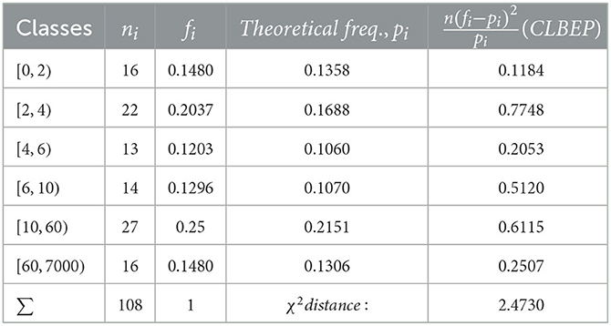
Table 1. Test for θ = 5.

TABLE 2

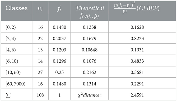
Table 2. Test for ${\widehat{\theta }}_1=5.0536$.

TABLE 3

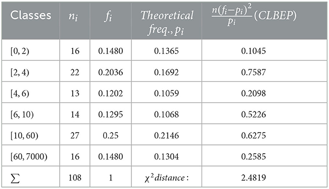
Table 3. Test for ${\widehat{\theta }}_2=4.9812$.

TABLE 4

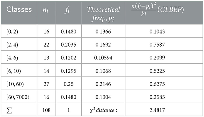
Table 4. Test for ${\widehat{\theta }}_3=4.9810$.

The χ² distances calculated for all the estimated values of the parameters are

$\begin{array}{l}{\chi }^{2}distance\left({\widehat{\theta }}_1\right)=2.4591\\ {\chi }^{2}distance\left({\widehat{\theta }}_2\right)=2.4819\\ {\chi }^{2}distance\left({\widehat{\theta }}_3\right)=2.4818.\end{array}$

The χ² test accepts the length-biased exponential Pareto model for all values of the parameter as expected, which $d^2\left({\widehat{\theta }}_1\right)$ is a minimum.

4.2. Goodness of fit

In this subsection, we apply the composite length-biased exponential-Pareto model to two real insurance data sets.

Data set I: is 100 Algerian (SAA company) fire insurance losses (see Appendix).

We provide in Table 5 the estimated value of fitted models and the values of the −LL, AIC, AICc, and BIC evaluated at the maximum-likelihood estimators.

TABLE 5

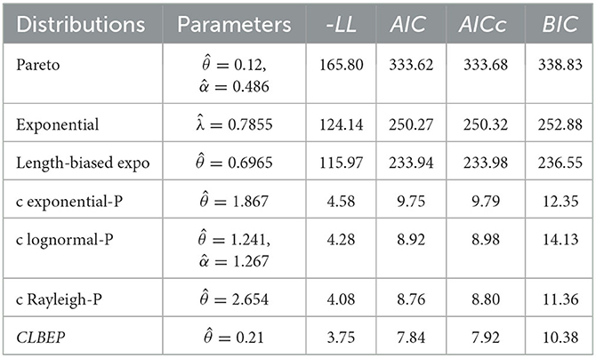
Table 5. Estimated values of fitted models and −LL, AIC, AICc, and BIC data set I.

Data set II: is 2, 156 Danish fire insurance losses.

We use the same analysis, we find

Tables 5, 6 indicate that the CLBEP model outperforms classical distributions, composite Rayleigh-Pareto, composite exponential-Pareto, and composite lognormal-Pareto models in terms of −LL, AIC, AICc, and BIC for data sets I and II. In addition, in data set II, the Pareto model outperforms the conventional model since it covers a larger loss (n = 2, 156).

TABLE 6

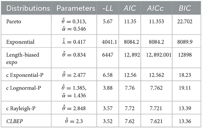
Table 6. Estimated values of fitted models and −LL, AIC, AICc, and BIC data set II.

5. Conclusion

A unique distribution known as the composite length-biased exponential Pareto generated is suggested for application. Some of the mathematical features of this distribution include the quantile function, stochastic ordering, moments of the CLBEP, and maximum-likelihood estimation. In contrast to other conventional and new composite distributions, the distribution proposed in this work gives very satisfactory results. The goodness of fit of this novel model is compared to different conventional and new composite models, such as composite exponential-Pareto, composite lognormal-Pareto, and composite Rayleigh-Pareto distributions, using two real fire insurance data sets (Algerian and Danish fire insurance losses). Compared to the standard models, the composite models provided a far better fit to the data. The composite exponential-Pareto, composite lognormal-Pareto, and composite Rayleigh-Pareto distributions do not fit as well as the CLBEP model provides. We predict that researchers interested in statistical sciences and their applications, such as dependability and actuarial sciences, will be drawn to the CLBEP model. A future research may examine the Bayesian estimation of the CLBEP parameter, introducing the truncated version of the CLBEP distribution. In addition, it is interesting to use similar composite distributions to model the epidemic problem.

Data availability statement

The original contributions presented in the study are included in the article/Supplementary material, further inquiries can be directed to the corresponding author.

Author contributions

All authors listed have made a substantial, direct, and intellectual contribution to the work and approved it for publication.

Acknowledgments

The authors acknowledge the Editor, FM and the referees of this journal for their constant encouragement to finalize the paper.

Conflict of interest

The authors declare that the research was conducted in the absence of any commercial or financial relationships that could be construed as a potential conflict of interest.

Publisher's note

All claims expressed in this article are solely those of the authors and do not necessarily represent those of their affiliated organizations, or those of the publisher, the editors and the reviewers. Any product that may be evaluated in this article, or claim that may be made by its manufacturer, is not guaranteed or endorsed by the publisher.

Supplementary material

The Supplementary Material for this article can be found online at: https://www.frontiersin.org/articles/10.3389/fams.2023.1137036/full#supplementary-material

References

1. Klugman SA, Panjer HH, Willmot G. Loss Models: From Data to Decisions. New York, NY: Wiley (2008).

Google Scholar

2. Liu B, Ananda MMA. Analyzing insurance data with an exponentiated composite Inverse-Gamma Pareto Model. Commun Stat Theory Methods. (2022) 2022:399. doi: 10.1080/03610926.2022.2050399

CrossRef Full Text | Google Scholar

3. Scollnik DPM. On composite Lognormal-Pareto models. Scand Actuarial J. (2007) 2007:20–33. doi: 10.1080/03461230601110447

CrossRef Full Text | Google Scholar

4. Benatmane, C, Zeghdoudi H, Shanker R, Lazri, N. Composite Rayleigh-Pareto distribution: application to real fire insurance losses data set. J Stat Manag Syst. (2021) 24:545–57. doi: 10.1080/09720510.2020.1759253

CrossRef Full Text | Google Scholar

5. Elbatal I, Aryal G. A new generalization of the exponential Pareto distribution. J Inf Optim Sci. (2017) 38:675–97. doi: 10.1080/02522667.2016.1220079

CrossRef Full Text | Google Scholar

6. EL-Sagheer RM, Mahmoud MAW, Abdallah SHM. Statistical inferences for new Weibull-Pareto distribution under an adaptive type-ii progressive censored data. J Stat Manag Syst. (2018) 21:1021–57. doi: 10.1080/09720510.2018.1467628

CrossRef Full Text | Google Scholar

7. Aminzadeh MS, Deng, M. Bayesian predictive modeling for Inverse Gamma-Pareto composite distribution. Commun Stat Theory Methods. (2019) 48:1938–54. doi: 10.1080/03610926.2018.1440595

CrossRef Full Text | Google Scholar

8. Cebrian A, Denuit M, Lambert PH. Generalized Pareto fit to the society of Actuaries' large claims database. North Am Actuarial J. (2003) 7:18–36. doi: 10.1080/10920277.2003.10596098

CrossRef Full Text | Google Scholar

9. Preda V, Ciumara R. On composite models: Weibull-Pareto lognormal-Pareto. A comparative study. Rom J Econ Forecast. (2006) 3:32–46.

Google Scholar

10. Cooray K, Ananda MA. Modeling actuarial data with a composite Lognormal-Pareto model. Scand Actuarial J. (2005) 5:321–34. doi: 10.1080/03461230510009763

CrossRef Full Text | Google Scholar

11. Teodorescu S, Vernic R. Some composite exponential-Pareto models for actuarial prediction. Rom J Econ Forecast. (2009) 12:82–100.

Google Scholar

12. Teodorescu S, Vernic R. On composite pareto models. Math Rep. (2013)15:11–29.

Google Scholar

13. Teodorescu S, Vernic R. A composite exponential–pareto distribution. The Annals of the “Ovidius” University of Constanta. Math Series. (2006) XIV:99–108.

Google Scholar