 Marc Bocquet
- CEREA, École des Ponts and EdF R&D, Île-de-France, France
The outstanding breakthroughs of deep learning in computer vision and natural language processing have been the horn of plenty for many recent developments in the climate sciences. These methodological advances currently find applications to subgrid-scale parameterization, data-driven model error correction, model discovery, surrogate modeling, and many other uses. In this perspective article, I will review recent advances in the field, specifically in the thriving subtopic defined by the intersection of dynamical systems in geosciences, data assimilation, and machine learning, with striking applications to physical model error correction. I will give my take on where we are in the field and why we are there and discuss the key perspectives. I will describe several technical obstacles to implementing these new techniques in a high-dimensional, possibly operational system. I will also discuss open questions about the combined use of data assimilation and machine learning and the short- vs. longer-term representation of the surrogate (i.e., neural network-based) dynamics, and finally about uncertainty quantification in this context.
1. Introduction
Computer vision and natural language processing have immensely benefited from the emergence of deep learning neural networks (NNs) and the availability of huge datasets over the past 15 years. It has long been recognized that arbitrarily large and deep NNs represent functional models for non-linear regressors [1]. But progresses in non-linear optimization due to a better derivation of the adjoint model1 and much richer datasets have allowed us to practically demonstrate the considerable potential of the approach [2, 3]. However, climate sciences (or more generally sciences of the atmosphere, oceans, land surfaces, their respective constituents, and biosphere) are far more error-prone and far less idealized than computer vision and natural language processing, which slowed down transfers between disciplines. The fabulous achievements of the methods nonetheless outweighed the hurdles, and the techniques finally percolated into the fields of geoscience.
Yet, geosciences have specificities. Modelers rely on comprehensive, though imperfect, scale-depend, costly numerical models, such as the dicretisation of the primitive equations for the geofluids. Earth scientists acquire and exploit huge observation datasets, but which do not offer full coverage of the system, neither in space nor in time. This challenge led to the development of data assimilation (DA) techniques that aim to optimally merge information from the observations and the numerical models to obtain a more accurate representation of the physical fields and parameters of the models.
Both machine learning (ML) to which deep learning belongs and DA are statistical estimation/inverse problems techniques which can offer predictions of the dynamical system under study and which share methodologies because they can both root in statistical and Bayesian principles. However, the acceleration of technical achievements, particularly the deep learning differentiable libraries, and its subsequent hype, made it very attractive to test ML techniques in geosciences. To address model deficiencies, which is critical for better forecasts and hindcasts, the emphasis is then more on data-driven rather than model-driven solutions.
In the following, I will first describe and justify this beneficial infusion of ideas to the geo- and climate sciences from a viewpoint at the intersection of the geoscientific dynamical systems, DA and ML. I will review some of the recent accomplishments through deep learning in the field, and in particular how the power of ML can be embedded in the Bayesian framework of DA, with a view to more accurate forecasts and surrogate modeling. I will give a realistic numerical example of a deep learning-based surrogate model for numerical weather prediction (NWP).
In the second part of this perspective paper, I will discuss aspects of these developments that may play a key role in the future success or represent significant challenges that must be addressed. I will first examine whether building a data-driven surrogate model requires focusing on very short-term dynamics (which amounts to equations discovery) or on longer-term dynamics (which amounts to building a surrogate resolvent of the dynamics). I will then return to the beneficial iterative combination of DA and ML to discover not only dynamics but also DA methods and their solver. I will then describe the potential of online vs. offline ML+DA schemes. As a third perspective, I will briefly discuss uncertainty quantification, where DA and ML can benefit from each other, before giving my final thoughts.
2. State-of-the-art
The Earth's climate is composed of several compartments with heterogeneous space and time scales: the atmosphere and its trace gases and aerosols, the oceans and its biological and chemical species, the land surface and its biosphere, the cryosphere (Arctic, Antarctic, Greenland, glaciers, and permafrost), etc. Its state and evolution, of critical importance for everyday life as well as the whole biosphere's fate, are estimated using numerical models of the geofluids and of the species' fate and using Earth's observation through constellations of satellites, ground stations, aircrafts, ships, buoys, radiosondes, and other remote sensors. Despite this impressive coverage, these observations remain noisy, can be non-local2, and can either be considered sparse or infrequent, depending on the instrument's platform and the Earth's compartment. Most geofluids are chaotic, which severely limits the Earth system's predictability. Predictions are computed through the optimal mathematical combination of these observations and the numerical forecasting models, i.e., DA, which has met success even beyond the boundaries of geoscience [5].
Note that the handling of these observations is a Big Data problem. At the same time, these numerical models are often computationally very demanding. They are orders of magnitude slower than the inference of large NNs. Thus, DA for operational numerical weather prediction is considered a high-performance computing challenge [6].
The precision of the forecasts is driven by the number of observations, their instrumental errors, as well as the fidelity of the numerical models. It is impacted by the relevance and consistency of the employed DA technique [7, 8]. It eventually depends on the accuracy of the sensitivity map established by the observation operator between the model variables and the observations, the so-called representation error [9].
Data assimilation in geosciences is the counterpart to training in ML and vice versa; they are both parts of estimation theory or inverse problems and combine a numerical model of either physical or statistical origin and possibly huge datasets (the larger, the better) [10]. There are known correspondences between them. For instance, the adjoint models [11] required by the gradients in variational DA draw from the branch of applied mathematics known as optimal control [12] and have been named backpropagation in deep learning [13]. They both ultimately rely on fine numerical optimization techniques. Yet, they diverge in their use of the model. In ML, the models are essentially statistical and fast to infer, while in DA, they are essential of physical origin and are usually significantly slower.
In contrast to computer vision and natural language processing which are well-delineated computer science problems, forecasting geophysical systems cannot be so neat a mathematical problem. Indeed, geophysical system have many sources of significant error mentioned above (model, data, and methods), they are often intrinsically multiscale and heterogeneous, and they are rarely isolated. Then, why should we bother with the recent progress of ML in computer vision and natural language processing if those could be specific and difficult to transfer to the climate sciences? The deep learning achievements are so spectacular that they cannot be ignored, nor are the reasons behind their success. Deep learning revived the NN techniques of the 90's by proving their relevance, by the availability of very large training databases, by demonstrating that deeper, i.e., multiple internal layers, and larger NNs can counter the curse of dimensionality of estimation theory, often met in ML and DA [14]. On a more technical level, this progress was critically accompanied by substantial software developments supported by Google, Facebook, Apache, Nvidia, etc. They propose open, easily accessible, and fast evolving deep learning libraries to efficiently implement the new methods on CPUs, GPUs, TPUs, and mobile/embedded devices. But the key ingredient is the ability of these software packages to generate the adjoint of any of the deep learning models, yielding differentiable models. This capability allows the generation of any loss function gradient relying on the NN model. Whether based on graph generation of the codes or eager execution (less numerically efficient but handling conditional branching in the code), they offer partial to almost complete remarkable solutions to the fundamental computational sciences problem of automatic differentiation. Examples of these tools are TensorFlow/Keras [15], PyTorch/Lightning [16], Jax [17], numpy, and autograd [18], which are mainly used on top of python or entirely new programming languages such as Julia/Flux [19].
In the meantime, over the past 20 years, progress has been slower in DA applied to the geosciences. Automatic differentiation was recognized as a critical challenge by this research community, especially since the advent and the remarkable success of the 4D-Var method and its implementation at the ECMWF, Météo-France, the UK MetOffice, Environment Canada, the Japan Meteorological office, and the Korean Meteorological Administration [20]. Researchers got help from computer scientists and experts in automatic differentiation but never got the means of the aforementioned high-tech companies. Besides, the presence of numerous physical thresholds (implemented via if statements in numerical geophysical codes) complicates the task As a consequence, the generation of adjoints was and can still be limited to key components of forecasting models and implemented by hand. This limitation significantly hampered the efforts to optimize key physical or statistical parameters of the DA and forecasting systems. Alternatives to variational-based DA methods exist, such as the ensemble Kalman filter [21–25]. They are excellent for forecasting but they are limited in their ability with non-linear higher-dimensional problems, where non-linear gradient-based optimization is the golden tool. Exceptions are iterative ensemble-variational techniques that mimic gradient-based optimization and, when numerically affordable, particle filters.
Because handling model error is key to making progress in geofluid forecasting, parameter estimation is also an important area of geophysical DA (e.g., [26]). Yet, efficient parameter estimation also relies on the ability to generate the adjoint of the models (whichever is present in the numerical chain from the parameters to the observations). Exceptions are some ensemble-variational techniques (e.g., a comparison of adjoint-based and iterative ensemble-based DA methods is given in [27]) but they come with their own problems such as time-dependent localization [28, 29]. As a consequence, efforts were also mitigated by this computer science issue.
As a result, deep learning techniques were welcomed into the geosciences. Among the first specialists to experiment with these techniques were the climatologists. They already have significant experience, if not advanced expertise in statistics and more traditional ML techniques. These techniques were applied to past events, reanalysis, and Coupled Model Intercomparison Project datasets, with decade-long forecast lead times, in contrast to the short-term geophysical forecasts where DA is deemed necessary. It was then proposed to apply advanced ML techniques to derive parameterizations of physical processes such as subgrid turbulent physics and convection, which are crucial for both accurate climate and shorter-term NWP models [30–34]. Over the past few years, in the realm of NWP and DA applied to the geosciences, deep learning was also seriously considered, with the research community shifting gears under ML influence. Obviously, it was partly due to the computer vision successes and legitimate exposure of these fashionable techniques. But my take is that the ML blood flow into NWP and DA is also due to other fundamental reasons. First, deep learning offers efficient non-linear regression tools that the DA community craves. Second, as mentioned earlier, the deep learning libraries offer solutions to the automatic differentiation core problem of DA, at the very least wherever NN architectures from these libraries are used, and with the promise to go beyond with Jax and Julia. Third, the possibilities offered by the deep learning methods and the related software freed our minds from many constraints and limitations of traditional DA-based parameter estimation. We can now attempt ambitious parameter estimation techniques, i.e., with millions of parameters non-linearly related to the observations and based on combined DA and deep learning. Moreover, this endeavor blurred the lines between NWP DA and ML experts in the geo- and climate sciences, making the community larger and its impact deeper with faster communication streams. Even ML/deep learning specialists from the industry attracted by the challenges of NWP and climate modeling brilliantly joined the collective efforts (e.g., Google, Nvidia, Huawei, and Microsoft [35–40]). Despite these references and the amazing accurate surrogate skills of their deep learning weather models, they still crucially rely on re-analysis data of the ECMWF patiently produced from complex and large physical models, huge datasets of meteorological observations, and increasingly sophisticated DA methods to combine them [41].
The following is focused on the recent and ongoing developments at the intersection of the dynamical systems in geoscience, DA and ML, that we (R. Arcucci's team at Imperial as well as mine) dubbed MLDADS for ML, DA, and dynamical systems. Despite the appearance of a niche subject, it reinvigorated past DA and ML open problems and witnessed a significant blooming of published works in geo- and environmental sciences (and beyond).
Let us list a few MLDADS opportunities and challenges aiming to combine DA and ML techniques. Deep learning can help us with subgrid parameterization as a powerful non-linear regression tool (e.g., [42, 43]). Most current parameterizations of geoscientific forecasting models are based on physical models with many tuned physical parameters. They alternatively rely on linear regressions, as for instance used in downscaling and upscaling [44]. Deep learning techniques hence offer more systematic non-linear regression tools provided that the datasets are large enough. More generally, it could help us with model error correction of forecasting systems [45–47]. Deep learning could help us build surrogate models of part or the whole dynamical systems either from pure observations or from data of high resolution simulations. In the first case, it bypasses the requirement for physical principles and modeling. In the second case, it can offer an acceleration to forecasting, or a way to simplify automatic differentiation of the represented physical model since its NN counterpart can easily be differentiated [48], or a fast means to generate ensembles, etc. It can also be a very appealing versatile tool to help with traditional DA methods, for instance in the tuning of statistical parameters needed to regularize covariances in ensemble DA methods, or help carry out non-linear adaptive transformation such as DA methods based on Gaussian anamorphosis.3
Creating data-driven surrogate models of low-order models of geofluids, which are meant to capture the key difficulties inherent to high-dimensional numerical models was one of the first objectives of the research community. There are by the end of 2022, dozens of ML papers in the literature dealing with the problem of data-driven surrogate dynamics, even if most of them focus on low-order models. The problem can be addressed by typical ML techniques, such as the projection on a regressor frame or basis, random forests, analogs, diffusion maps, reservoir computing, long short-term memory NN, and other NN approaches (e.g., [49–59]).
However, most ML techniques assume almost noiseless and complete observations which are fundamental limitations to extrapolating them to the geosciences. By contrast, most DA methods can handle noisy and sparse observations. That is why surrogate modeling in this context can be tackled using a conjunction of ML and DA techniques to exploit noisy and incomplete observations such as those met in realistic geoscience systems [60–64]. For high-dimensional systems, the relative lack of information can be mitigated by additionally using past trajectories or information on the system such as an approximate model derived from physical laws [65–67].
In a variational context, the mathematical problem of estimating the dynamical model and the state trajectory can be framed into a rigorous Bayesian formalism [60–63, 68–70]. Generalizing a classical short-window DA rational [71] yields a cost function for variational DA, where ML tools are leveraged upon:
where is the observations operator at time k, is the resolvent of the statistical dynamical model, typically a NN with weights and biases stacked in the p vector; the yk and xk for k = 0, …, K are the observation and the state vectors of the physical system over the time interval [0, K], respectively. The matrices Rk and Qk are the observation and model error covariance matrices, respectively. The background term −2ln p(p, x0), which corresponds to the prior density function on the initial condition x0 and the parameters p, is neglected here for the sake of simplicity. Besides, the sensitivity to x0 vanishes in the large K limit for chaotic dynamics, a standpoint at variance with classical DA where K is small and regularization of p is usually addressed via a stopping criterion built on the validation loss and dropout layers (although a Tikhonov term is also sometimes summoned). Accounting for this approximation, is given up to terms that do not depend on p and xk.
This cost function is rigorously obtained from Bayes' rule under Gaussian assumptions on some of the errors of the problem. This resembles a typical weak-constraint 4D-Var cost function [72]. This DA standpoint is remarkable as it allows for noisy and partial observations of the physical system, whereas most ML approaches do not account for this significantly noisy and partial data. Note that the solution of this problem is a trajectory for the state over the time interval, a deterministic NN model parameterized by p⋆, and a stochastic correction over the deterministic surrogate model, whose predefined statistics is normal with model error covariance matrix Qk. It is possible to partially estimate this stochastic correction through the expectation-maximization algorithm (see [62, 73, 74]).
Let us assume that the dynamics to be learned fully and directly observed, i.e., Hk ≡ I, and that the observation errors vanish, i.e., Rk → 0. Then the observation term in the cost function gets frozen and imposes that xk ≃ yk, so that, in this limit, becomes
This cost function coincides with a typical ML loss function provided Qk ≡ I.
Note that it is also possible to accomplish the same goal of joint estimation using ensemble-based DA methods [75, 76]. It then appears as a much more ambitious parameter estimation problem than in traditional DA. It has however a potentially higher numerical complexity than the variational approach. In particular, the size of the ensemble may have to match the number of global parameters plus the number of a single copy of the local parameters, in addition to careful use of localization to regularize ensemble-based covariances.
3. Perspectives
Let us discuss a selection of important open questions of the domain.
3.1. Physical and statistical hybrid models and their resolvent vs. tendency corrections
Learning the full dynamics of the atmosphere or the ocean, not to mention a holistic Earth system model from pure observations to build a surrogate dynamical model could be possible but would not yet compete with state-of-the-art physical models. An intermediate, reasonable step would be to use a hybrid representation of the dynamics. In this framework, the statistical data-driven model is a correction to a well-tuned physical numerical model [65, 66, 77, 78]. For instance, the partial differential equations of the physical model could be corrected, i.e., the tendencies using NWP terminology:
where x ↦ φ(x) is the physical tendency and x ↦ n(p, x) is the tendency correction. Alternatively, one could correct the resolvent which would be a substitute for the statistical model in the cost function :
where x ↦ Φ(x) is the resolvent obtained from the physical model whereas is the corrective statistical model. When possible, this hybrid formulation has the key advantages of (i) limiting the number of NN parameters, (ii) providing the learning step with the physical model as a first guess, and consequently (iii) accelerating the learning step. Hence, this approach has been favored in several recent and ambitious surrogate models. One potential issue can appear if the adjoint of the physical model is not available. In that case, the tendencies cannot be learned through non-linear optimization; only the resolvent approach would be easily implementable since it would not require the physical model's adjoint. In both cases, the NN correction's adjoint is obtained by automatic differentiation. These options for learning corrections of chaotic models are still largely unexplored.
Finally, note that surrogate modeling of geofluids has a lot of connections with, and could gain from recent surrogate modeling endeavors, in computational fluid dynamics and engineering (e.g., [79–82]).
3.2. MLDADS optimization system
An algorithm proposed to minimize as defined in Equation (1), on both the state trajectory and the statistical NN model parameters consists of iteratively (i) estimating the state trajectory using classical DA methods with (ii) optimizing the NN parameters using ML methods [61]. This is illustrated in Figure 1. A DA smoother (e.g., 4D-Var, ensemble-based smoothers) is typically used in the DA step while deep learning is used in the ML step. This has been reckoned mathematically as a coordinate descent for non-linear optimization, with iterations of the loop until convergence [62]. Moreover, it has been demonstrated to be successful with low-order models [62]. Nonetheless, this could seem numerically costly for higher dimensional problems, such as NWP, so that one should first focus on the first half steps of this loop. In this framework, traditional DA can be considered as order–1/2 of the loop, while order–1, i.e., DA followed by ML has been studied in [78] and coincides with model error correction using analysis increments of DA runs. Note that the notation order–1/2 merely means that DA only represents half of the loop, the first step out of two in the surrogate model estimation. This has the potential to be used in an NWP context, since the analysis increments are natural outputs of operational DA. Order–3/2 consists in additionally using the NN model error correction of the order–1 loop to improve NWP based on DA with an improved forecast model [78]. This in turn means uncovering a state trajectory closer to the true one which, in realistic conditions, cannot be accessed directly since the observations are both sparse and noisy. It certainly remains to implement these in an NWP framework. If order–2 (and beyond) has been proven to be consistent and have a lot of potential for low-order models [62], it would be interesting to demonstrate this potential with higher dimensional models and NWP. This entails a second application of ML, and hence obtaining a more accurate surrogate model or model error correction in the hybrid case. Nonetheless, this is expected to be a significant numerical challenge.
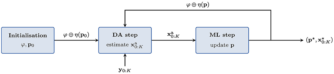
Figure 1. Schematic of the coordinate descent alternating DA and ML which aims to minimize and is expected to converge to the maximum a posteriori estimator. φ represents the physical model, η is the deep learning model that depends on parameters p, and φ ⊕ η(p) is the hybrid model.
One idea would be to skip the estimation of the state trajectory, or marginalizing it out, and hence to compute the sensitivity of the observations with respect to the parameters directly. This idea is put forward by the Ensemble Kalman Inversion technique [83] and has been experimented with but on a small number of parameters [84]. It remains to be investigated whether the method can be applied to larger sets of parameters, or even deep learning NNs. This approach would likely call for model reduction, explicitly or implicitly, which would be implemented by deep learning.
Figure 2 illustrates learning the dynamics of the global atmosphere from the ERA5 dataset [41]. We used the setup, data, and ECMWF Integrated Forecasting System model runs provided by the WeatherBench platform [85]. A residual deep NN model of about 1.5 × 10⁶ parameters is learned from 38 years of meteorology at coarse 5.625° × 5.625° spatial resolution. This surrogate model is independently tested on the years 2017–2018 over many forecast runs, on the 500 hPa geopotential fields using the root mean square error (RMSE) and the auto-correlation (ACC), as functions of the forecast lead time up to 14 days. The surrogate model uses 3 levels of geopotential and 3 levels of temperature. Its forecast skill is compared to global and daily climatologies, to the persistence model, and to the ECMWF model at truncation T42 (about 2.8° grid-cell at the equator). We observe that in spite of its coarser resolution (about T21 truncation), the surrogate model outperforms the ECMWF model at T42 projected on T21. The shades around the skill curves represent the variability of the forecast scores induced by the variability of the ERA5 meteorology over the test years 2017–2018, which is in turn mostly decided by the distribution of initial states on (part of) the current attractor of the chaotic dynamics and by forcings (radiation, ocean). They were obtained by running 5, 000 forecasts in the test period starting from as many distinct initial conditions and computed from the dispersion of this ensemble of forecasts. Provided the surrogate model is a good enough representation of the truth, this variability is not expected to depend much on the surrogate model solution, since it is mainly driven by the dynamics.4 Surprisingly, this uncertainty (or risk of the forecast scores) is usually not provided in the ML surrogate modeling literature, where the focus is only on deterministic forecasts without their uncertainty.
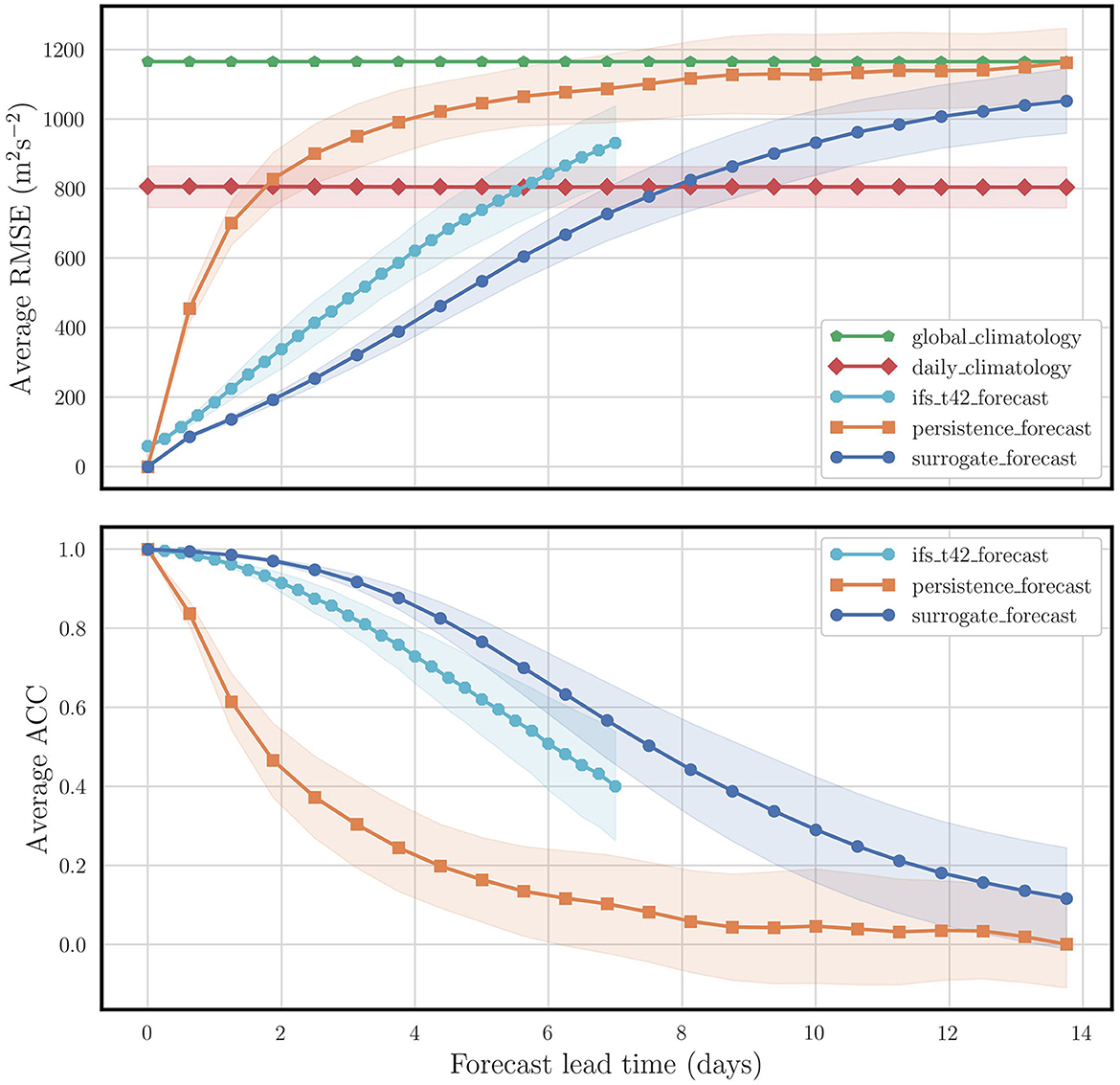
Figure 2. RMSE (top) and ACC (bottom) for the 500 hPa geopotential predicted by the learned neural network model that simulates weather at coarse resolution, and comparison to uniform and daily climatologies, persistence, and the ECMWF model forecasts at T42 (see text for details).
Among the fundamental open problems in combining DA with ML is the ability of the ML+DA schemes to assimilate fresh observations. Upon receiving them, one would update our knowledge of not only the state and possibly a few physical model parameters (as in classical DA) but would also update any neural network used within the sequential algorithm, whether it is related to correcting the evolution model, the observation model, or any block of the assimilation scheme itself. In other words, one wishes to obtain from online/sequential ML+DA algorithms what has been achieved in offline variational ML+DA. This challenge has been explored with low-dimensional to intermediate models with ensemble Kalman filters [75, 76] and with variational schemes [67, 78] where the model (or a compartment thereof) and the state trajectory were both updated when new observations are acquired. We expect this topic to thrive in the coming years since (i) it aligns with the conditions of operational forecasting centers, (ii) it proposes algorithms for incremental learning over very long periods of time where data are generated/acquired, and since (iii) later observations better capture the current trends in a time-dependent model in the context of climate change.
A more systemic approach to applying ML tools on DA is to learn the DA scheme itself. This clearly requires that the building blocks of the DA scheme be differentiable so that gradients with respect to the outputs of the DA scheme, typically the analysis products, could be efficiently computed [86–88]. Such a typical holistic approach has been coined end-to-end in ML. Learning the output of a local ensemble Kalman filter in conjunction with the intermediate global circulation model SPEEDY was proposed very early [89, 90]. A radically different approach consists in optimizing the internal cogs of DA schemes by finding an efficient latent space representation for either the ensemble Kalman filter [91–94] or the variational schemes [95]. One can also try to learn the solvers of, for instance, variational schemes since these are critical to the DA analysis and its numerical efficiency and cost [96, 97]. Beyond supplementing ML techniques to DA schemes as was originally proposed, one may further replace key components of the DA scheme with advanced NNs such as transformers and multi-headed attention [98]. Possibilities of combining ML and DA from this end-to-end standpoint seems endless as hinted at by the previous examples. But the existence of a more powerful, unifying and enlightening way to do so is still to be investigated.
3.3. Uncertainty quantification
Uncertainty quantification, i.e., the ability to quantify the confidence we have in one of our statistical estimator, is in the genes of DA and NWP. In particular, most DA methods have an underlying Bayesian rationale that helps to formalize or connect to uncertainty quantification. Ensemble Kalman filtering and ensemble-variational methods in geoscience are based on an ensemble of states, or state trajectories because ensembles provide an estimate of the uncertainty of the state trajectory through the ensemble spread and other empirical moments. The confidence in weather forecasts is assessed with ensemble forecasts which could be initialized with the ensemble from an ensemble Kalman filter [99]. However, uncertainty quantification with variational DA methods is challenging since it requires estimating a Hessian in high dimension, which is a dreadful task. There are nowadays several methods meant to address this, such as an ensemble of DA for sequential DA [100, 101], approximating the Hessian of cost functions [102], or randomized singular value decomposition [103, 104]. Finally, model error estimation is one of the most critical issues of DA in geoscience [115, and references therein].
For the same reason, uncertainty quantification in basic ML is far from natural and simple. Besides, it does not have the same rigorous basis as in DA despite seminal papers that paved the way (e.g., [105, 106]) but were insufficiently followed. However, a wealth of solutions have been proposed, most of them unsatisfactory in view of the standards of uncertainty quantification. Some of them underwent a preliminary investigation in geoscience. First of all, learning models from several random initializations of the weights and biases and from distinct randomization of the data, hence generating a deep ensemble, yields some measure of uncertainty quantification for the statistical model per se and its internal parameters through e.g., generating an ensemble of model variants [107]. But this quantification is unlikely to match, or even target, the uncertainty of surrogate model estimates. Indeed, those perturbations of the weights and biases are not sampled according to their conditional likelihood. Dropout layers are used as a regularization scheme which, through the increased robustness to noise in the NN, mitigates overfitting. Optimizing these layers is a priori used in the learning step while they are kept frozen in the inference (i.e., the forecasts). Yet, again, the technique should in general fail to target the uncertainty of the estimate [108]. Additionally, stochasticity can be introduced again in the forecasts to build an ensemble [107, 109, 110]. Whether this generated ensemble is a proper quantification of uncertainty is however questionable. Alternatively, one can try to augment the NN and predict statistical hyperparameters such as the standard deviation of the variable estimates, or some parameters of their a priori statistics. This is reminiscent of variational auto-encoders where the hyperparameters nonetheless lie in the bottleneck layer. Yet, such an approach is much more difficult to train [111]. Indeed, those hyperparameters would be at the second level in a Bayesian hierarchy and requires more testing and investigations. At the first hierarchy level, the NN could output biases [112]. Another approach consists of estimating probability density functions of some of the output variables (marginals), using a softmax layer for a categorical output of the density or a convolutional layer for a continuous density [110]. More generally, one could account for the weights uncertainty by including them as part of the outputs, using Bayes' rule, an approach even closer to the principles of DA. These NNs are Bayesian neural networks [113]. Even though basic ML does not genuinely account for uncertainty, it is hoped that the flexibility of deep learning will allow designing augmented architectures that address uncertainty quantification. Yet, the subject remains in its infancy in ML. It could benefit from the seminal papers of the field [105, 106] and from the expertise developed on Bayesian uncertainty quantification within geophysical and in particular meteorological DA. Finally, let us highlight out that the subject is complementary to all of the topics mentioned in Section 3.2.
4. Final thoughts
In the previous section, a few key MLDADS challenges have been examined. The field is nonetheless evolving very fast. So where does this lead us?
I believe supplementing DA with the power of ML tools is already a success and, as a topic, should continue to thrive for many years, boosting DA research, with still many applications to explore. Furthermore, the DA+ML topic may not have clear boundaries yet; the merging of DA and ML is at the beginning.
On the one hand, model error correction and surrogate modeling, which is at the core of MLDADS, undergo much faster progress than when they were only addressed by pure DA and dynamical systems techniques. On the other hand, they rely on either high-resolution simulations of existing models or from re-analysis, a product of DA techniques, observation, and numerical modeling. As recently proven by the industry artificial intelligence research teams and others, the potential of surrogate modeling for short-term meteorological forecasting is extraordinary but critically relies on the modelers' expertise through the reanalysis products. That is why a long-term challenge in the geoscience domain is to build surrogate models from large database of observations only, without relying on physical and numerical expertise which, for now, remains critical.
Moreover, the potential of such dynamical surrogate modeling for longer time-scales, i.e., for climate modeling, is far from established and the topic is nascent (e.g., [114]). Accounting for slow-evolving trends and limited time reanalysis data from a climate standpoint as opposed to numerical weather prediction, is likely to make the surrogate and model error correction challenges quite difficult.
Data availability statement
Publicly available datasets were analyzed in this study. This data can be found here: https://github.com/pangeo-data/WeatherBench.
Author contributions
The author confirms being the sole contributor of this work and has approved it for publication.
Funding
This work was granted access to the HPC resources of IDRIS under the allocations 2020-AD011011184R1 and 2021-AD011011184R2 made by GENCI; this was used for generating Figure 2 of the manuscript.
Acknowledgments
The author would like to acknowledge the many useful suggestions of two reviewers on the manuscript. The author would also like to express his gratitude to the many colleagues with whom he has collaborated on the topic or who offered their insight: A. Farchi, A. Carrassi, J. Brajard, L. Bertino, M. Bonavita, P. Laloyaux, M. Chrust, T. Janjić, T. S. Finn, C. Durand, J. Dumont Le Brazidec, P. Vanderbecken, R. Fablet, S. Ouala, P. Tandéo, R. Arcucci, S, Gratton, S. Penny, and I. Szunyogh. CEREA is a member of the Institut Pierre-Simon Laplace (IPSL).
Conflict of interest
The author declares that the research was conducted in the absence of any commercial or financial relationships that could be construed as a potential conflict of interest.
Publisher's note
All claims expressed in this article are solely those of the authors and do not necessarily represent those of their affiliated organizations, or those of the publisher, the editors and the reviewers. Any product that may be evaluated in this article, or claim that may be made by its manufacturer, is not guaranteed or endorsed by the publisher.
Footnotes
1. ^More precisely, the adjoint operator of the sensitivity of the model output to the input variables.
2. ^Non-local observations are typically linear or non-linear functions of spatially extended variables. Typical examples in the geosciences are the radiance measurements of space-born instruments which often probe full columns of the atmosphere. See for instance The Frontiers' Research Topic Data Assimilation of Non-local Observations in Complex Systems [4].
3. ^Daisuke Hotta, communication at ISDA online 2021.
4. ^In particular, this variability is not the uncertainty attached to the learning process from the dataset. However, it shows how easy it is to pick initial conditions with flattering forecast scores.
References
4. Hutt A, Bocquet M, Carrassi A, Lei L, Potthast R. Editorial: data assimilation of nonlocal observations in complex systems. Front Appl Math Stat. (2021) 7:658272. doi: 10.3389/fams.2021.658272
5. Carrassi A, Bocquet M, Bertino L, Evensen G. Data assimilation in the geosciences: an overview on methods, issues, and perspectives. WIREs Climate Change. (2018) 9:e535. doi: 10.1002/wcc.535
6. Bauer P, Quintino T, Wedi N, Bonanni A, Chrust M, Deconinck W. The ECMWF Scalability Programme: Progress Plans. ECMWF (2020). Available online at: https://www.ecmwf.int/node/19380
7. Magnusson L, Källén E. Factors influencing skill improvements in the ECMWF forecasting system. Monthly Weather Rev. (2013) 141:3142–53. doi: 10.1175/MWR-D-12-00318.1
8. Bauer P, Thorpe A, Brunet G. The quiet revolution of numerical weather prediction. Nature. (2015) 525:47–55. doi: 10.1038/nature14956
9. Janjić T, Bormann N, Bocquet M, Carton JA, Cohn SE, Dance SL, et al. On the representation error in data assimilation. Q J R Meteorol Soc. (2018) 144:1257–78. doi: 10.1002/qj.3130
10. Geer AJ. Learning earth system models from observations: machine learning or data assimilation? Philos Trans R Soc A. (2021) 379:20200089. doi: 10.1098/rsta.2020.0089
12. Le Dimet FX, Talagrand O. Variational algorithms for analysis and assimilation of meteorological observations: theoretical aspects. Tellus A. (1986) 38:97–110. doi: 10.1111/j.1600-0870.1986.tb00459.x
13. Baydin AG, Pearlmutter BA, Radul AA, Siskind JM. Automatic differentiation in machine learning: a survey. J Mach Learn Res. (2018) 18:5595–637.
14. Bocquet M, Pires CA, Wu L. Beyond Gaussian statistical modeling in geophysical data assimilation. Monthly Weather Rev. (2010) 138:2997–3023. doi: 10.1175/2010MWR3164.1
15. Abadi M, Agarwal A, Barham P, Brevdo E, Chen Z, Citro C, et al. TensorFlow: large-scale machine learning on heterogeneous systems. arXiv preprint arXiv:1603.04467 (2015).
16. Paszke A, Gross S, Massa F, Lerer A, Bradbury J, Chanan G, et al. PyTorch: an imperative style, high-performance deep learning library. In: Advances in Neural Information Processing Systems 32. Curran Associates, Inc. (2019). p. 8024–35.
17. Bradbury J, Frostig R, Hawkins P, James Johnson M, Leary C, Maclaurin D. JAX: Composable Transformations of Python+NumPy Programs (2018). Available online at: http://github.com/google/jax
18. Maclaurin D, Duvenaud D, Adams RP. Autograd: effortless gradients in numpy. In: ICML 2015 AutoML Workshop. (2015).
19. Bezanson J, Edelman A, Karpinski S, Shah VB. Julia: a fresh approach to numerical computing. SIAM Rev. (2017) 59:65–98. doi: 10.1137/141000671
20. Rabier F, Järvinen H, Klinker E, Mahfouf JF, Simmons A. The ECMWF operational implementation of four-dimensional variational assimilation. I: experimental results with simplified physics. Q J R Meteorol Soc. (2000) 126:1143–70. doi: 10.1002/qj.49712656415
21. Evensen G. Sequential data assimilation with a nonlinear quasi-geostrophic model using Monte Carlo methods to forecast error statistics. J Geophys Res. (1994) 99:10143–62. doi: 10.1029/94JC00572
22. Burgers G, van Leeuwen PJ, Evensen G. Analysis scheme in the ensemble Kalman filter. Monthly Weather Rev. (1998) 126:1719–24. doi: 10.1175/1520-0493(1998)126<1719:ASITEK>2.0.CO;2
23. Evensen G, van Leeuwen PJ. An ensemble Kalman smoother for nonlinear dynamics. Monthly Weather Rev. (2000) 128:1852–67. doi: 10.1175/1520-0493(2000)128<1852:AEKSFN>2.0.CO;2
24. Asch M, Bocquet M, Nodet M. Data Assimilation: Methods, Algorithms, and Applications Fundamentals of Algorithms. Philadelphia, PA: SIAM (2016).
25. Evensen G, Vossepeol FC, van Leeuwen PJ. Data Assimilation Fundamentals: A Unified Formulation of the State and Parameter Estimation Problem. Cham: Springer International Publishing (2022).
26. Hansen JA, Penland C. On stochastic parameter estimation using data assimilation. Phys D. (2007) 230:88–98. doi: 10.1016/j.physd.2006.11.006
27. Bocquet M, Sakov P. Joint state and parameter estimation with an iterative ensemble Kalman smoother. Nonlinear Process Geophys. (2013) 20:803–18. doi: 10.5194/npg-20-803-2013
28. Bocquet M, Sakov P. An iterative ensemble Kalman smoother. Q J R Meteorol Soc. (2014) 140:1521–35. doi: 10.1002/qj.2236
29. Bocquet M. Localization and the iterative ensemble Kalman smoother. Q J R Meteorol Soc. (2016) 142:1075–89. doi: 10.1002/qj.2711
30. Brenowitz ND, Bretherton CS. Prognostic validation of a neural network unified physics parameterization. Geophys Res Lett. (2018) 45:6289–98. doi: 10.1029/2018GL078510
31. Gentine P, Pritchard M, Rasp S, Reinaudi G, Yacalis G. Could machine learning break the convection parameterization deadlock? Geophys Res Lett. (2018) 45:5742–51. doi: 10.1029/2018GL078202
32. Jiang GQ, Xu J, Wei J. A deep learning algorithm of neural network for the parameterization of Typhoon-ocean feedback in Typhoon forecast models. Geophys Res Lett. (2018) 45:3706–16. doi: 10.1002/2018GL077004
33. O'Gorman PA, Dwyer JG. Using machine learning to parameterize moist convection: potential for modeling of climate, climate change, and extreme events. J Adv Model Earth Syst. (2018) 10:2548–63. doi: 10.1029/2018MS001351
34. Reichstein M, Camps-Valls G, Stevens B, Denzler J, Carvalhais N, Prabhat. Deep learning and process understanding for data-driven Earth system science. Nature. (2019) 566:195–204. doi: 10.1038/s41586-019-0912-1
35. Ravuri S, Lenc K, Willson M, Kangin D, Lam R, Mirowski P, et al. Skilful precipitation nowcasting using deep generative models of radar. Nature. (2021) 597:672–7. doi: 10.1038/s41586-021-03854-z
36. Keisler R. Forecasting global weather with graph neural networks. arXiv preprint arXiv:220207575 (2022). doi: 10.48550/arXiv.2202.07575
37. Pathak J, Subramanian S, Harrington P, Raja S, Chattopadhyay A, Mardani M, et al. FourCastNet: a global data-driven high-resolution weather model using adaptive Fourier neural operators. arXiv preprint arXiv:2202.11214 (2022). doi: 10.48550/arXiv.2202.11214
38. Bi K, Xie L, Zhang H, Chen X, Gu X, Tian Q. Pangu-Weather: a 3D high-resolution model for fast and accurate global weather forecast. arXiv preprint arXiv:2211.02556 (2022). doi: 10.48550/arXiv.2211.02556
39. Lam R, Sanchez-Gonzalez A, Willson M, Wirnsberger P, Fortunato M, Pritzel A, et al. GraphCast: learning skillful medium-range global weather forecasting. arXiv preprint arXiv:2212.12794 (2022). doi: 10.48550/arXiv.2212.12794
40. Nguyen T, Brandstetter J, Kapoor A, Gupta JK, Grover A. ClimaX: a foundation model for weather and climate. arXiv preprint arXiv:2301.10343 (2023). doi: 10.48550/arxiv.2301.10343
41. Hersbach H, Bell B, Berrisford P, Hirahara S, Horanyi A, Munoz-Sabater J, et al. The ERA5 global reanalysis. Q J R Meteorol Soc. (2020) 146:1999–2049. doi: 10.1002/qj.3803
42. Bolton T, Zanna L. Applications of deep learning to ocean data inference and subgrid parameterization. J Adv Model Earth Syst. (2019) 11:376–99. doi: 10.1029/2018MS001472
43. Zanna L, Bolton T. Deep learning of unresolved turbulent ocean processes in climate models. In: Deep Learning for the Earth Sciences: A Comprehensive Approach to Remote Sensing, Climate Science, and Geosciences. John Wiley & Sons Ltd (2021). p. 298–306.
44. Barthélémy S, Brajard J, Bertino L. Super-resolution data assimilation. Ocean Dyn. (2022) 72:661–78. doi: 10.1007/s10236-022-01523-x
45. Watson PAG. Applying machine learning to improve simulations of a chaotic dynamical system using empirical error correction. J Adv Model Earth Syst. (2019) 11:1402–17. doi: 10.1029/2018MS001597
46. Bonavita M, Laloyaux P. Machine learning for model error inference and correction. J Adv Model Earth Syst. (2020) 12:e2020MS002232. doi: 10.1029/2020MS002232
47. Chen TC, Penny SG, Whitaker JS, Frolov S, Pincus R, Tulich S. Correcting systematic and state-dependent errors in the NOAA FV3-GFS using neural networks. J Adv Model Earth Syst. (2022) 14:e2022MS003309. doi: 10.1029/2022MS003309
48. Hatfield S, Chantry M, Dueben P, Lopez P, Geer A, Palmer T. Building tangent-linear and adjoint models for data assimilation with neural networks. J Adv Model Earth Syst. (2021) 13:e2021MS002521. doi: 10.1029/2021MS002521
49. Brunton SL, Proctor JL, Kutz JN. Discovering governing equations from data by sparse identification of nonlinear dynamical systems. Proc Natl Acad Sci USA. (2016) 113:3932–7. doi: 10.1073/pnas.1517384113
50. Lguensat R, Tandeo P, Ailliot P, Pulido M, Fablet R. The analog data assimilation. Monthly Weather Rev. (2017) 145:4093–107. doi: 10.1175/MWR-D-16-0441.1
51. Harlim J. Data-Driven Computational Methods: Parameter and Operator Estimations. Cambridge: Cambridge University Press (2018).
52. Pathak J, Hunt B, Girvan M, Lu Z, Ott E. Model-free prediction of large spatiotemporally chaotic systems from data: a reservoir computing approach. Phys Rev Lett. (2018) 120:024102. doi: 10.1103/PhysRevLett.120.024102
53. Dueben PD, Bauer P. Challenges and design choices for global weather and climate models based on machine learning. Geosci Model Dev. (2018) 11:3999–4009. doi: 10.5194/gmd-11-3999-2018
54. Fablet R, Ouala S, Herzet C. “Bilinear residual neural network for the identification and forecasting of dynamical systems,” In: EUSIPCO 2018, European Signal Processing Conference. Rome (2018). p. 1–5.
55. Champion K, Lusch B, Kutz JN, Brunton SL. Data-driven discovery of coordinates and governing equations. Proc Natl Acad Sci USA. (2019) 116:22445–51. doi: 10.1073/pnas.1906995116
56. Scher S, Messori G. Generalization properties of feed-forward neural networks trained on Lorenz systems. Nonlinear Process Geophys. (2019) 26:381–99. doi: 10.5194/npg-26-381-2019
57. Weyn JA, Durran DR, Caruana R. Using deep learning to predict gridded 500-hPa geopotential height from historical weather data. J Adv Model Earth Syst. (2019) 11:2680–93. doi: 10.1029/2019MS001705
58. Arcomano T, Szunyogh I, Pathak J, Wikner A, Hunt BR, Ott E. A machine learning-based global atmospheric forecast model. Geophys Res Lett. (2020) 47:e2020GL087776. doi: 10.1029/2020GL087776
59. Nadiga BT. Reservoir computing as a tool for climate predictability studies. J Adv Model Earth Syst. (2021) 13. doi: 10.1029/2020MS002290
60. Bocquet M, Brajard J, Carrassi A, Bertino L. Data assimilation as a learning tool to infer ordinary differential equation representations of dynamical models. Nonlinear Process Geophys. (2019) 26:143–62. doi: 10.5194/npg-26-143-2019
61. Brajard J, Carrassi A, Bocquet M, Bertino L. Combining data assimilation and machine learning to emulate a dynamical model from sparse and noisy observations: a case study with the Lorenz 96 model. J Comput Sci. (2020) 44:101171. doi: 10.1016/j.jocs.2020.101171
62. Bocquet M, Brajard J, Carrassi A, Bertino L. Bayesian inference of chaotic dynamics by merging data assimilation, machine learning and expectation-maximization. Found Data Sci. (2020) 2:55–80. doi: 10.3934/fods.2020004
63. Arcucci R, Zhu J, Hu S, Guo YK. Deep data assimilation: integrating deep learning with data assimilation. Appl Sci. (2021) 11:1114. doi: 10.3390/app11031114
64. Gottwald GA, Reich S. Supervised learning from noisy observations: combining machine-learning techniques with data assimilation. Phys D. (2021) 423:132911. doi: 10.1016/j.physd.2021.132911
65. Wikner A, Pathak J, Hunt B, Girvan M, Arcomano T, Szunyogh I, et al. Combining machine learning with knowledge-based modeling for scalable forecasting and subgrid-scale closure of large, complex, spatiotemporal systems. Chaos. (2020) 30:053111. doi: 10.1063/5.0005541
66. Brajard J, Carrassi A, Bocquet M, Bertino L. Combining data assimilation and machine learning to infer unresolved scale parametrisation. Philos Trans R Soc A. (2021) 379:20200086. doi: 10.1098/rsta.2020.0086
67. Farchi A, Bocquet M, Laloyaux P, Bonavita M, Malartic Q. A comparison of combined data assimilation and machine learning methods for offline and online model error correction. J Comput Sci. (2021) 55:101468. doi: 10.1016/j.jocs.2021.101468
68. Hsieh WW, Tang B. Applying neural network models to prediction and data analysis in meteorology and oceanography. Bull Am Meteor Soc. (1998) 79:1855–70.
69. Abarbanel HDI, Rozdeba PJ, Shirman S. Machine learning: deepest learning as statistical data assimilation problems. Neural Comput. (2018) 30:2025–55. doi: 10.1162/neco_a_01094
70. Penny SG, Smith TA, Chen TC, Platt JA, Lin HY, Goodliff M, et al. Integrating recurrent neural networks with data assimilation for scalable data-driven state estimation. J Adv Model Earth Syst. (2022) 14:e2021MS002843. doi: 10.1029/2021MS002843
71. Lorenc AC. Modelling of error covariances by 4D-Var data assimilation. Q J R Meteorol Soc. (2003) 129:3167–82. doi: 10.1256/qj.02.131
72. Trémolet Y. Accounting for an imperfect model in 4D-Var. Q J R Meteorol Soc. (2006) 132:2483–504. doi: 10.1256/qj.05.224
73. Ghahramani Z, Roweis ST. Learning nonlinear dynamical systems using an EM algorithm. In:Kearns M, Solla S, Cohn D, , editors. Advances in Neural Information Processing Systems. vol. 11. MIT Press; (1999) p. 431–7.
74. Nguyen VD, Ouala S, Drumetz L, Fablet R. EM-like learning chaotic dynamics from noisy and partial observations. arXiv preprint arXiv:190310335 (2019).
75. Bocquet M, Farchi A, Malartic Q. Online learning of both state and dynamics using ensemble Kalman filters. Found Data Sci. (2021) 3:305–30. doi: 10.3934/fods.2020015
76. Malartic Q, Farchi A, Bocquet M. State, global, and local parameter estimation using local ensemble Kalman filters: applications to online machine learning of chaotic dynamics. Q J R Meteorol Soc. (2022) 148:2167–93. doi: 10.1002/qj.4297
77. Pathak J, Wikner A, Fussell R, Chandra S, Hunt BR, Girvan M, et al. Hybrid forecasting of chaotic processes: using machine learning in conjunction with a knowledge-based model. Chaos. (2018) 28:041101. doi: 10.1063/1.5028373
78. Farchi A, Laloyaux P, Bonavita M, Bocquet M. Using machine learning to correct model error in data assimilation and forecast applications. Q J R Meteorol Soc. (2021) 147:3067–84. doi: 10.1002/qj.4116
79. Raissi M, Perdikaris P, Karniadakis GE. Physics-informed neural networks: a deep learning framework for solving forward and inverse problems involving nonlinear partial differential equations. J Comput Sci. (2019) 378:686–707. doi: 10.1016/j.jcp.2018.10.045
80. Karniadakis GE, Kevrekidis IG, Lu L, Perdikaris P, Wang S, Yang L. Physics-informed machine learning. Nat Rev Phys. (2021) 3:422–40. doi: 10.1038/s42254-021-00314-5
81. Vinuesa R, Brunton SL. Enhancing computational fluid dynamics with machine learning. Nat Comput Sci (2022) 2:358–66. doi: 10.1038/s43588-022-00264-7
82. Kochkov D, Smith JA, Alieva A, Wang Q, Brenner MP, Hoyer S. Machine learning-accelerated computational fluid dynamics. Proc Natl Acad Sci USA. (2021) 118:e2101784118. doi: 10.1073/pnas.2101784118
83. Kovachki NB, Stuart AM. Ensemble Kalman inversion: a derivative-free technique for machine learning tasks. Inverse Probl. (2019) 35:095005. doi: 10.1088/1361-6420/ab1c3a
84. Schneider T, Lan S, Stuart A, Teixeira J. Earth system modeling 2.0: a blueprint for models that learn from observations and targeted high-resolution simulations. Geophys Res Lett. (2017) 44:12396–417. doi: 10.1002/2017GL076101
85. Rasp S, Dueben PD, Scher S, Weyn JA, Mouatadid S, Thuerey N. Weatherbench: a benchmark data set for data-driven weather forecasting. J Adv Model Earth Syst. (2020) 12:e2020MS002203. doi: 10.1029/2020MS002203
86. Andrychowicz M, Denil M, Gómez S, Hoffman MW, Pfau D, Schaul T, et al. Learning to learn by gradient descent by gradient descent. In:Lee D, Sugiyama M, Luxburg U, Guyon I, Garnett R, , editors. Advances in Neural Information Processing Systems. vol. 29. Curran Associates, Inc. (2016). p. 3981–9.
87. Hospedales T, Antoniou A, Micaelli P, Storkey A. Meta-learning in neural networks: a survey. IEEE Trans Pattern Anal Mach Intell. (2021) 44:5149–69. doi: 10.1109/TPAMI.2021.3079209
88. Liu R, Ma L, Yuan X, Zeng S, Zhang J. Task-oriented convex bilevel optimization with latent feasibility. IEEE Trans Image Process. (2022) 31:1190–203. doi: 10.1109/TIP.2022.3140607
89. Cintra RS, de Campos Velho HF. Global data assimilation using artificial neural networks in SPEEDY model. In: 1st International Symposium Uncertainty Quantification and Stochastic Modeling. São Sebastião (2012). p. 648–54.
90. Cintra RS, de Campos Velho HF. Data assimilation by artificial neural networks for an atmospheric general circulation model. In:ElShahat A, , editor. Advanced Applications for Artificial Neural Networks. IntechOpen (2018). p. 265–86. doi: 10.5772/intechopen.70791
91. Boudier P, Fillion A, Gratton S, Gürol S. DAN – An optimal Data Assimilation framework based on machine learning recurrent networks. arxiv preprint arxiv:2010.09694. (2020).
92. Ouala S, Nguyen D, Drumetz L, Chapron B, Pascual A, Collard F, et al. Learning latent dynamics for partially observed chaotic systems. Chaos (2020) 30:103121. doi: 10.1063/5.0019309
93. Peyron M, Fillion A, Gürol S, Marchais V, Gratton S, Boudier P, et al. Latent space data assimilation by using deep learning. Q J R Meteorol Soc. (2021) 147:3759–77. doi: 10.1002/qj.4153
94. Revach G, Shlezinger N, Ni X, Escoriza AL, Van Sloun RJ, Eldar YC. KalmanNet: neural network aided Kalman filtering for partially known dynamics. IEEE Trans Signal Process. (2022) 70:1532–47. doi: 10.1109/TSP.2022.3158588
95. Optimal reduced space for variational data assimilation. J Comp Phys. (2019) 379:51–69. doi: 10.1016/j.jcp.2018.10.042
96. Fablet R, Chapron B, Drumetz L, Mémin E, Pannekoucke O, Rousseau F. Learning variational data assimilation models and solvers. J Adv Model Earth Syst. (2021) 13:e2021MS002572. doi: 10.1029/2021MS002572
97. Fablet R, Febvre Q, Chapron B. Multimodal 4DVarNets for the reconstruction of sea surface dynamics from SST-SSH synergies. arXiv preprint arXiv:220701372 (2022). doi: 10.48550/arXiv.2207.01372
98. Finn TS. Self-attentive ensemble transformer: representing ensemble interactions in neural networks for earth system models. arXiv preprint arXiv:210613924 (2021).
99. Bowler NE. Comparison of error breeding, singular vectors, random perturbations and ensemble Kalman filter perturbation strategies on a simple model. Tellus A. (2006) 58:538–48. doi: 10.1111/j.1600-0870.2006.00197.x
100. Raynaud L, Berre L, Desroziers G. An extended specification of flow-dependent background error variances in the Météo-France global 4D-Var system. Q J R Meteorol Soc. (2011) 137:607–19. doi: 10.1002/qj.795
101. Bonavita M, Raynaud L, Isaksen L. Estimating background-error variances with the ECMWF ensemble of data assimilation system: some effects of ensemble size and day-to-day variability. Q J R Meteorol Soc. (2011) 137:423–34. doi: 10.1002/qj.756
102. Bousserez N, Henze DK, Perkins A, Bowman KW, Lee M, Liu J, et al. Improved analysis-error covariance matrix for high-dimensional variational inversions: application to source estimation using a 3D atmospheric transport model. Q J R Meteorol Soc. (2015) 141:1906–21. doi: 10.1002/qj.2495
103. Desroziers G, Brousseau P, Chapnik B. Use of randomization to diagnose the impact of observations on analyses and forecasts. Q J R Meteorol Soc. (2005) 131:2821–37. doi: 10.1256/qj.04.151
104. Farchi A, Bocquet M. On the efficiency of covariance localisation of the ensemble Kalman filter using augmented ensembles. Front Appl Math Stat. (2019) 5:3. doi: 10.3389/fams.2019.00003
105. MacKay DJC. A practical Bayesian framework for backpropagation networks. Neural Comput. (1992) 4:448–72. doi: 10.1162/neco.1992.4.3.448
106. Andrieu C, de Freitas N, Doucet A, Jordan MI. An introduction to MCMC for machine learning. Mach Learn. (2003) 50:5–43. doi: 10.1023/A:1020281327116
107. Scher S, Messori G. Ensemble methods for neural network-based weather forecasts. J Adv Model Earth Syst. (2021) 13:e2020MS002331. doi: 10.1029/2020MS002331
108. Osband I. Risk versus uncertainty in deep learning: bayes, bootstrap and the dangers of dropout. In: NIPS Workshop on Bayesian Deep Learning. (2016).
109. Gal Y, Ghahramani Z. Dropout as a Bayesian approximation: representing model uncertainty in deep learning. In:Balcan MF, Weinberger KQ, , editors. Proceedings of The 33rd International Conference on Machine Learning. New York, NY: PMLR (2016). p. 1050–9.
110. Clare MCA, Jamil O, Morcrette CJ. Combining distribution-based neural networks to predict weather forecast probabilities. Q J R Meteorol Soc. (2021) 147:4337–57. doi: 10.1002/qj.4180
111. Garg S, Rasp S, Thuerey N. WeatherBench probability: a benchmark dataset for probabilistic medium-range weather forecasting along with deep learning baseline models. arXiv preprint arXiv:220500865 (2022). doi: 10.48550/arXiv.2205.00865
112. Grönquist P, Yao C, Ben-Nun T, Dryden N, Dueben P, Li S, et al. Deep learning for post-processing ensemble weather forecasts. Philos Trans R Soc A. (2021) 379:20200092. doi: 10.1098/rsta.2020.0092
113. Blundell C, Cornebise J, Kavukcuoglu K, Wierstra D. Weight uncertainty in neural network. In:Bach F, Blei D, , editors. Proceedings of the 32nd International Conference on Machine Learning. Lille: PMLR (2015). p. 1613–22.
114. Arcomano T, Szunyogh I, Wikner A, Hunt BR, Ott E. A hybrid atmospheric model incorporating machine learning can capture dynamical processes not captured by its physics-based component. ESS Open Arch. (2022). doi: 10.22541/essoar.167214579.97903618/v1
Keywords: numerical weather prediction, climate, deep learning, geosciences, machine learning, data assimilation, surrogate model, artificial neural networks
Citation: Bocquet M (2023) Surrogate modeling for the climate sciences dynamics with machine learning and data assimilation. Front. Appl. Math. Stat. 9:1133226. doi: 10.3389/fams.2023.1133226
Received: 28 December 2022; Accepted: 06 February 2023;
Published: 06 March 2023.
Edited by:
Axel Hutt, Inria Nancy - Grand-Est Research Centre, FranceReviewed by:
Geir Evensen, Norwegian Research Institute (NORCE), NorwayPeter Jan Van Leeuwen, Colorado State University, United States
Copyright © 2023 Bocquet. This is an open-access article distributed under the terms of the Creative Commons Attribution License (CC BY). The use, distribution or reproduction in other forums is permitted, provided the original author(s) and the copyright owner(s) are credited and that the original publication in this journal is cited, in accordance with accepted academic practice. No use, distribution or reproduction is permitted which does not comply with these terms.
*Correspondence: Marc Bocquet, bWFyYy5ib2NxdWV0QGVucGMuZnI=